Corn Residue Covered Area Mapping with a Deep Learning Method Using Chinese GF-1 B/D High Resolution Remote Sensing Images

Abstract

Black soil is one of the most productive soils with high organic matter content. Crop residue covering is important for protecting black soil from alleviating soil erosion and increasing soil organic carbon. Mapping crop residue covered areas accurately using remote sensing images can monitor the protection of black soil in regional areas. Considering the inhomogeneity and randomness, resulting from human management difference, the high spatial resolution Chinese GF-1 B/D image and developed MSCU-net+C deep learning method are used to mapping corn residue covered area (CRCA) in this study. The developed MSCU-net+C is joined by a multiscale convolution group (MSCG), the global loss function, and Convolutional Block Attention Module (CBAM) based on U-net and the full connected conditional random field (FCCRF). The effectiveness of the proposed MSCU-net+C is validated by the ablation experiment and comparison experiment for mapping CRCA in Lishu County, Jilin Province, China. The accuracy assessment results show that the developed MSCU-net+C improve the CRCA classification accuracy from IOU_AVG = 0.8604 and Kappa_AVG = 0.8864 to IOU_AVG = 0.9081 and Kappa_AVG = 0.9258 compared with U-net. Our developed and other deep semantic segmentation networks (MU-net, GU-net, MSCU-net, SegNet, and Dlv3+) improve the classification accuracy of IOU_AVG/Kappa_AVG with 0.0091/0.0058, 0.0133/0.0091, 0.044/0.0345, 0.0104/0.0069, and 0.0107/0.0072 compared with U-net, respectively. The classification accuracies of IOU_AVG/Kappa_AVG of traditional machine learning methods, including support vector machine (SVM) and neural network (NN), are 0.576/0.5526 and 0.6417/0.6482, respectively. These results reveal that the developed MSCU-net+C can be used to map CRCA for monitoring black soil protection.

1. Introduction

The black soil region is one of the most productive soils with fertile soils, characterized by a thick, dark-colored soil horizon rich in organic matter [1], and soil types include black soil, kastanozems, chernozem, meadow soil, and dark brown soil, etc. There are black soil and chernozem mainly in the study area, which plays a vital role in guaranteeing national food security in China [2]. Nevertheless, soil fertility decreased quickly in recent years for the reason of human activities and ecological systems changing. Compared with before reclamation, the organic matter content of black soil in Northeast China decreased 50%~60% [3]. To protect the precious black soil, the conservational tillage is developed and carried out in China. One meaningful way is the crop residue left for covering the black soil within the nongrowing season [4]. The crop residue covering can mitigate water erosion and wind erosion, increase the organic matter content by letting the organic matter of crop residue back to the soil [5]. In addition, the minimum soil disturbance can be used to prevent the destruction of farmland soil layers to ensure the expected growth of crops [6]. Therefore, whether or not there is crop residue covered in the soil surface is very important for black soil protection [7]. Unfortunately, the traditional methods for identifying the crop residual covered area are time-consuming and laborious, which can’t be carried out in regional areas, quickly and timely.

Remote sensing is an efficient way to capture the land surface information quickly in regional areas [8,9]. The crop residue cover estimation and the conservative tillage monitoring based on remote sensing data have become a topic of significant interest to researchers [10,11]. In the past few decades, a series of methods have been proposed for estimating local and regional crop residue cover using remote sensing data, including the linear spectral unmixing [12], the spectral index [13,14], and the triangle space technique [15]. However, remote sensing techniques to estimate crop residue cover has been limited by the variations of moisture in the crop residue and soil [16]. For example, linear spectral unmixing techniques that use fixed crop residue and soil endmember spectra may lead to inaccurate estimation resulting from the difficulty in determining the abundance of pure crop residue spectral constituents. [17]. The cellulose and lignin absorption features are attenuated as moisture content increases, which decreases the accuracy of crop residue cover estimation using existing spectral index methods [10]. The problem of the triangle space technique lies in the difficulty of acquiring hyperspectral images, which limits the application of this method for estimating crop residue cover on a large-scale [15]. These studies are all about crop residue cover estimation using remote sensing data, disregarding the residue cover type (i.e., residue covering directly, stalk-stubble breaking, stubble standing, etc.). The residue cover type mapping is very significant for crop residue cover estimation for carrying out conservation tillage and crop residue quantity estimation for clean energy production. Therefore, this study focuses on regional crop residue cover mapping using high spatial resolution Chinese GF-1 B/D images.

Texture features are the essential characteristics of high spatial resolution remote sensing images, which are very useful for fine mapping of small and irregular land surface targets [18]. Image texture analysis refers to measuring heterogeneity in the distribution of gray values within a given area [19]. There is abundant spatial information of crop residue covered area from high spatial resolution remote sensing images. Mining the texture features will contribute to improving the accuracy of mapping crop residue covered areas. Some researchers developed some algorithms to extract spatial and shape features, including rotation invariance [20], texture statistics [21], and mathematical morphology [22]. Moreover, these mid-level features mostly rely on setting some free parameters subjectively, which cannot mine the abundant spatial and textural information provided by high spatial resolution remote sensing images [23]. Therefore, a more thorough understanding of the textural and spatial features is required for mapping crop residue covered areas that are scattered and irregular.

The fine spatial resolution and abundant textural information of high spatial resolution remote sensing images can’t work fully using traditional supervised classification methods. The traditional segmentation methods, such as turbopixel/superpixel segmentation, watershed segmentation, and active contour models, also have their own drawbacks. Specifically, turbopixel/superpixel segmentation methods [24,25] are subject to both under-segmentation and irregularly shaped superpixel boundaries. Watershed segmentation method [26,27] is fast in image segmentation, but the number and compactedness of superpixels cannot be controlled. Active contour models [28,29] cannot work well for the object with obvious multiple colors. Fortunately, deep learning semantic segmentation methods are developing rapidly in the field of computer vision and classification of remote sensing images [30,31]. In general, there are two kinds of semantic pixel-based classification methods, including patch-based and end-to-end in the convolutional neural network (CNN) architectures. The drawback of the patch-based classification method [32] lies in that the trained network can only predict the central pixel of the input image, resulting in low classification effectiveness. Moreover, the end-to-end framework methods [33,34,35,36] are usually known as semantic segmentation networks, which became more popular for the advantages of their high process effectiveness, discovering the contextual features, and learning representativeness and distinguishing features automatically. The U-Net is a typical semantic segmentation network with a contracting path to capture context and a symmetric expanding path, which is a lightweight network and can be trained end-to-end and get-well results in segmentation of neuronal structures [37]. Therefore, there are many improved networks based on UNET. Including combined with residual connections, atrous convolutions, pyramid scene parsing pooling [38], and re-designed skip pathways [39]. In addition, the attention mechanism, multiscale convolution group (MSCG), and depth-wise separable convolution can improve network performance effectively proved by Woo et al. [40], Chen et al. [41], and Chen et al. [42]. These semantic segmentation network models with end-to-end structures are trained not only further excavate the relationship between the spectral and the label, but also to learn the contextual features.

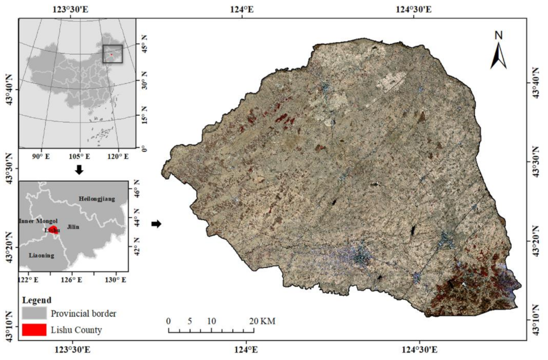
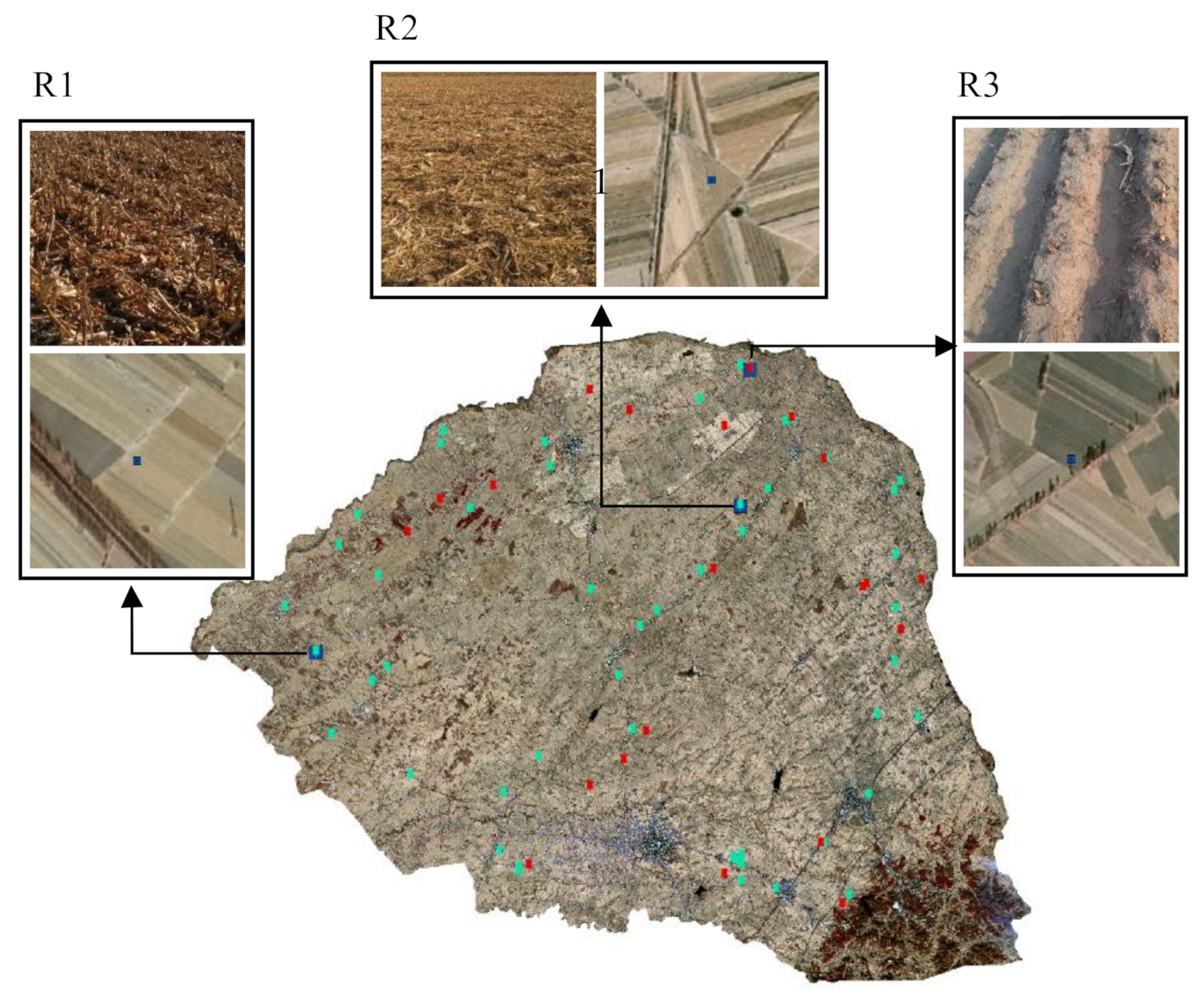
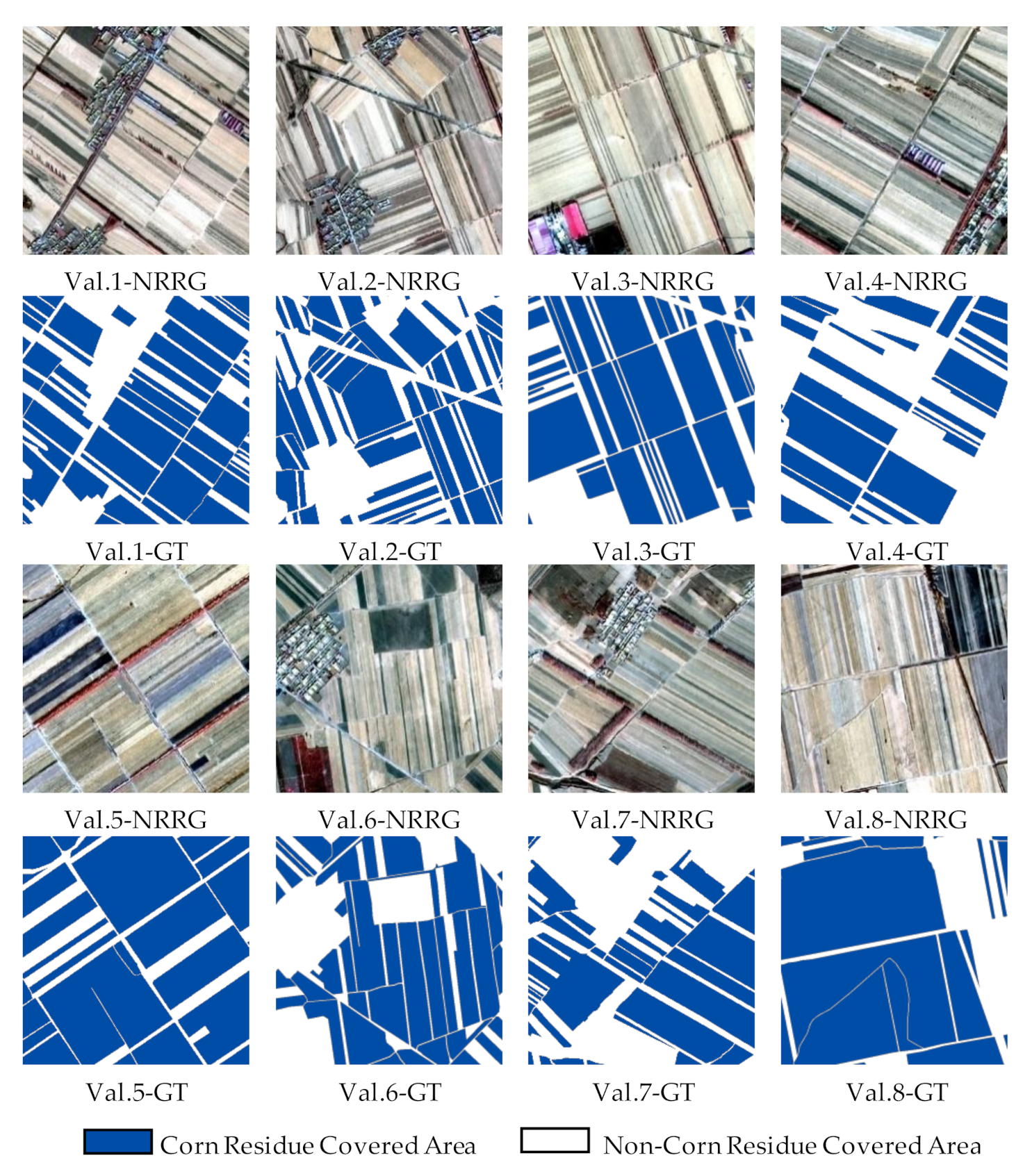
There are many kinds of different crop residue cover type in Lishu County, Siping City, Jilin Province, including residue covering directly, stalk-stubble breaking, stubble standing, where is a typical study area for crop residue cover mapping. Lishu County is located in the Golden Corn Belt of black soil in Northeast China, and there is a 93% cultivated area is planted corn. Lishu County is a typical area of corn residue covering for protecting black soil. Therefore, this study focuses on mapping corn residue covered area (CRCA) using the deep learning method based on GF-1 B/D high resolution remote sensing images. The conservation tillage is defined by The Conservation Technology Information Center (CTIC) as any tillage and planting system that has the residue cover is greater than 30% after planting [43,44]. Therefore, we define the CRCA as corn residues cover more significantly than 30%, and the depth semantic segmentation method is chosen for mapping the CRCA. 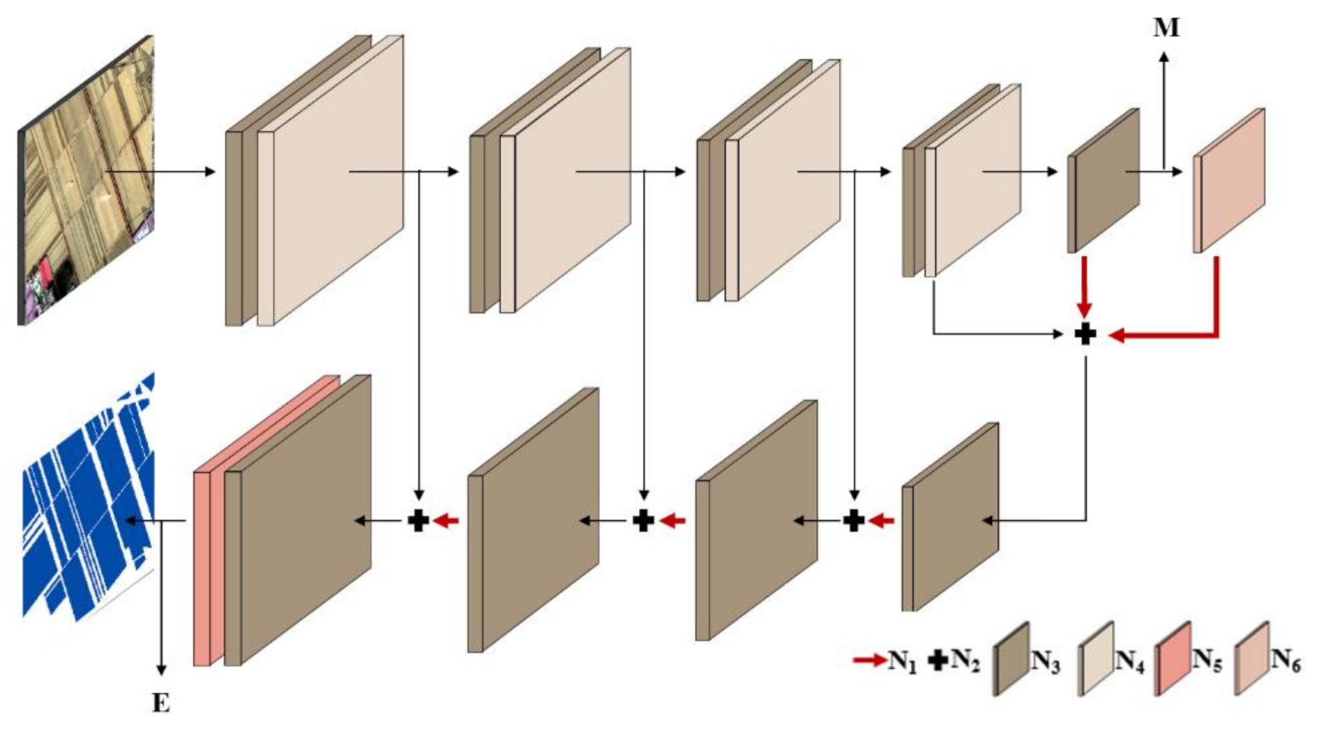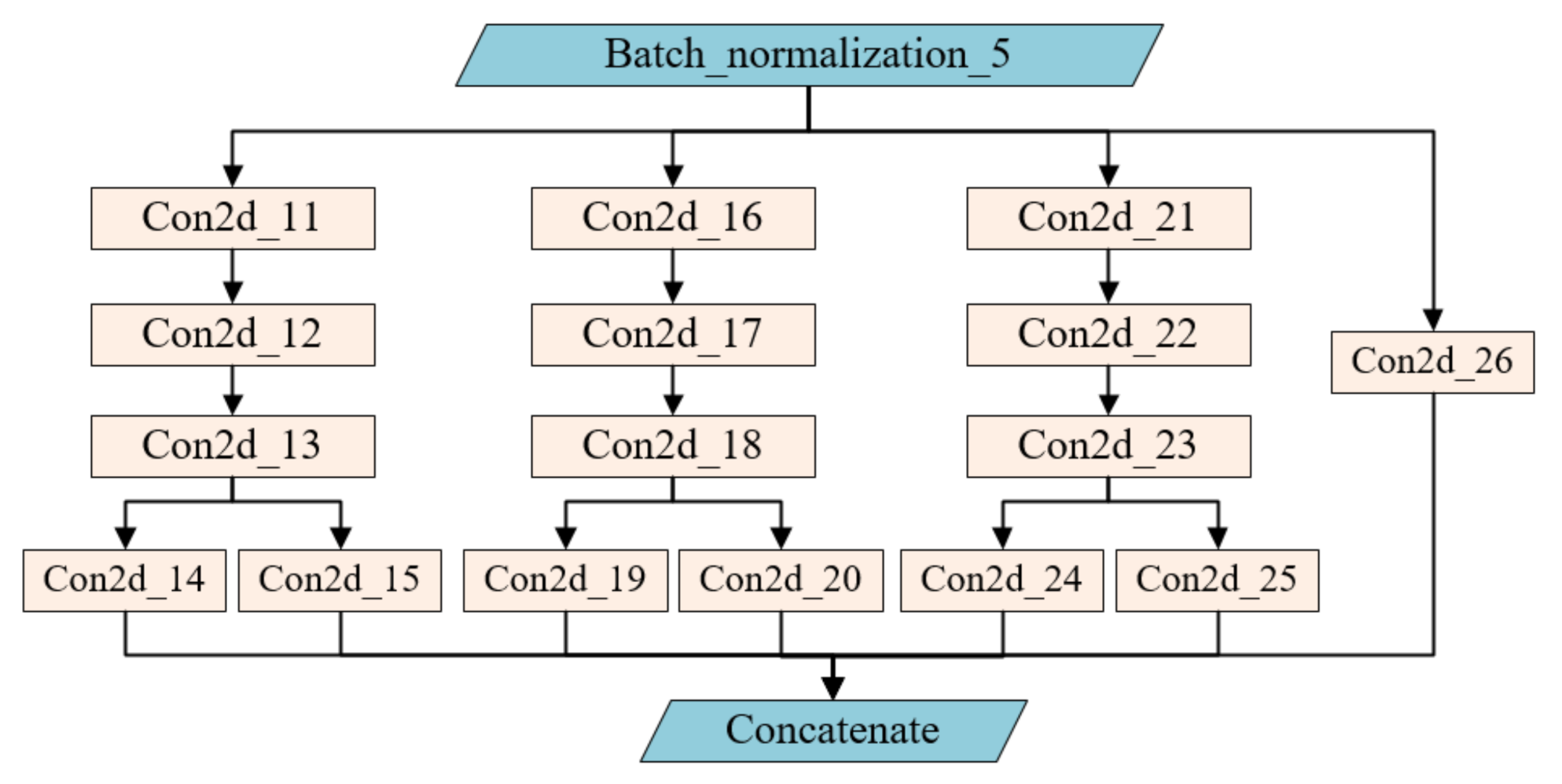Full Connected Conditional Random Field (FCCRF) [45] is a discriminative undirected graph learning model, which can fully consider the global information and structural information, and can optimize the classification results by combining MSCU-net and FCCRF. With the proposed method, the automatic mapping of CRCA from GF1 B/D high resolution remote sensing images is developed in this study. The novelties of this study are as followed. (1) A designed network MSCU-net is developed for exploring the spatial features of high resolution images by combing the U-Net with multiscale convolution group (MSCG), the global loss function, and Convolutional Block Attention Module (CBAM). (2) The FCCRF is combined with MSCU-net to construct MSCU-net+C to further optimizing CRCA to alleviate the noise in high spatial resolution results images. (3) Exploring the potential of Chinese GF1 B/D high resolution remote sensing images for mapping the CRCA accurately and automatically.

This study is structured as followed. In the next section, we introduce the study area and the data collection for corn residue cover firstly. In Section 3, the details of our designed network architecture and assessment indexes are presented. Then, we compared different improvements strategies, different classifiers with the proposed method to prove its effectiveness on GF-1 B/D images, and the classification results in Section 4. Next, the discussions about the strengths and weaknesses of the proposed method with respect to other relevant studies are given in Section 5. Finally, considerations for future work and the conclusions of the study are presented in Section 6.

2. Study Area and Data Collection

2.1. Study Area

The study area is Lishu County, which is located in the southwest of Jilin Province, China, ranging from 123°45′–124°53′E and 43°02′–43°46′N (Figure 1). Lishu County is in the inner Golden Corn Belts of Northeast China, located in the Black Soil of Northeast China, which is one of the worldwide well-known Four Black Soil Belts. It covers approximately 4209 km², and it is the main crop cultivated area and a grain-producing center in China. The terrain is high in the southeast with low hills, low in the northwest, and flat in the middle with wavy plains. The study area is the alluvial plain resulting from the Dongliao River in the north.

For protecting the precious black soil, the Conservation Tillage is developed in Lishu County in 2007. This lets the crop residues left in the field cover black soil and strip tillage by crisscrossing residue covering area and tillage area. The crop residues covering can keep the soil from being exposed. Crop residues covering can not only alleviate soil erosion, but also preserve the evaporation of soil water and fertilizer for increasing the soil fertility gradually. The main crop planted in the study area is corn, with a small number of soybeans, peanuts, peppers, and other crops. If the black soil is covered by crop residues in the nongrowing season is vital for protecting black soil. Therefore, identifying the CRCA accurately is very important for monitoring the conservation tillage application for protecting black soil.

2.2. Data Collection

2.2.1. Acquisition of Remote Sensing Images

The Chinese GF-1 B/C/D satellites were launched on 31 March 2018, with a high temporal resolution of 4 days and high spatial resolution of 2 m for the panchromatic band and 8 m for multispectral bands. The multispectral bands include red, green, blue, and near-infrared bands, and the imaging width is 66 km. Therefore, the GF-1 B/C/D remote sensing images are chosen for mapping the CRCA in this study. The corn is sown at the end of April, and is harvested in early October in the study area. There is the most corn residue left in the field after harvest at the end of October and November. Then the cloudless GF-1 D image (central longitude124.03/central latitude 43.55) was acquired on 8 November 2020, and GF-1 B image (central longitude124.7/central latitude 43.46) acquired on 13 November 2020, are used to identify the CRCA in Lishu County. The mosaic GF-1 B/D image after pan-sharping is as Figure 2. The band information of GF-1 B/D image is shown in

Table 1. Band information of GF-1 B/D image.

Bands	Spectral Range	Spatial Resolution	Revisit Cycle
Panchromatic	450–900 nm	2 m	4 days
Blue	450–520 nm	8 m
Green	520–590 nm
Red	630–690 nm
Near-Infrared	770–890 nm

.

2.2.2. Field Data Collection

To validate the residue covered area mapping accuracy, the field campaign was done from 6 November to 14 November 2020, for surveying the fields covered by corn residue. The crop residue covered area in Lishu County can be classified into two groups: High residue covered area with coverage is greater than 30%, and low residue covered area with coverage is less than 30%. This threshold of 30% is used to decide if it is conservative tillage. There are 69 samplings collected, in total, for in-field campaigns, and the spatial distribution of them is shown in Figure 2. The labels of Figure 2 are as followed: R1 and R2 represent corn high stubble residue covered area and short-stubble residue covered area, respectively. The residue coverage of R1 and R2 is greater than 30%, they are the residue covered area to be extracted consequently, which is labeled green. R3 represents the corn stubble covered area where the residue coverage is less than 30%, which should not be extracted in this study, which is labeled red.

3. Method

There is great success has been achieved in land cover classification [46] and crop planted area classification [47] by the current U-Net architecture of deep learning methods. The Convolutional Neural Networks (CNN), based on the U-Net architecture (Ronneberger et al., 2015), are used to identify the CRCA in this study, and the architecture of which is as Figure 3. U-net is a U-shaped convolutional neural network, which consists of the encoder part from down-sampling and decoder part from up-sampling. The down-sampling encoder network is stacked from 3 × 3 convolution operator and ReLU (Nair & Hinton, 2010) nonlinear activation function. With the deepening of the network layer, the encoder network performs down-sampling and increases the number of convolution channels for extracting higher-level features of bigger receptive fields. The up-sampling decoder network is used to recover the resolution of outputs and produce classification results. The shallow information of the down-sampling network can bring more detailed boundary information. Therefore, the U-net is suitable for the classification of objects with fewer pixels. However, it is difficult to decide whether each feature information is necessary for the large number of parameters in each layer of U-Net. Therefore, we develop some improvements based on the origin U-Net architecture. In order to improve the network training performance and optimize the model parameters, MSCG and a loss function are constructed in the middle layer of the network, and CBAM is introduced in the upper layer to design an MSCU-net network. The architecture of the network is depicted in Section 3.1. In order to prevent overfitting, the network is optimized, which is introduced in Section 3.2. The FCCRF method was used to optimize the classification results, which are introduced in Section 3.3, and the accuracy evaluation methods are illustrated in Section 3.4.

3.1. Network Architecture

An MSCU-net method is designed to identify CRCA, which architecture is illustrated in Figure 3. It is a typical encoder–decoder architecture that is used to encode the abundant contextual information and decode to recover the detailed boundaries of land surface objects effectively. The architecture consists of 36 convolution layers, four pooling layers, and one sigmoid function, where the N3 convolution group is made up of the repeated application of two 3 × 3 convolutions, batch normalization, and a rectified linear unit activation function. The whole networks are divided into nine parts by the N3 convolution group. The number of the first five convolution kernels increases gradually with the sequence of 64, 128, 256, 512, 1024. The MSCG is applicable to obtain more abundant spatial texture features for remote sensing images in the middle layer. Then the intermediate layer loss function M is added in the fifth part for optimizing the network parameters. The MSCG is composed of multiscale convolution, including 16 convolutions layers, and the output convolution kernel number is 1024. The features of MSCG and the fifth N3 convolution output are up-sampled through a 2 × 2 window, which are fused with the fourth pooling feature for the first time. During the fusing process, the first fusion feature is up-sampled by a 2 × 2 window, and the second fusion feature is obtained by combining with the third pooling feature. In the same way, the third and the fourth fusion features are acquired. The attention module includes a two-dimensional convolution, and the CBAM (Convolutional Block Attention Module) module is added after the ninth N3 convolution group. The ninth N3 convolution group is acquired automatically by the weight of the feature map through learning to enhance features and suppress redundant features. Finally, the output features of CBAM are processed by one-dimensional convolution and sigmoid activation function. The feature maps with the same size as the original image are output to achieve end-to-end pixel-based prediction of the original image.

3.1.1. Attention Mechanism

It is well known that attention plays a vital role in human perception [48], human beings can quickly scan the global information of the objects or scene for capturing the region of interest, and then pay more attention to the area of interest [49]. The attention mechanism in deep learning is essentially similar to the human attention mechanism, which is used to capture the critical information of ongoing classification tasks from the massive information of deep learning. The attention model is used widely in various deep learning tasks, including semantic segmentation and objects detection. It is one of the critical technologies in deep learning that deserves the most attention and in-depth understanding.

CBAM is an effective and uncomplicated module, which is illustrated in Figure 4. The CBAM can be integrated into any CNNs architectures seamlessly with negligible overheads, which is end-to-end trainable along with base CNNs [50]. CBAM, coupled by channel attention module (CAM) and spatial attention module (SAM) in series structure, is introduced and embedded into the end of MSCU-net architecture to achieve end-to-end training—it is beneficial to obtain more important information in the process of CRCA classification for improving the identification accuracy. The feature map F is given as input, F_s is the final output, which is the output feature map through SAM. The matrix dimension sizes of F and F_s are all C × H × W. The following formula can express the attention process:

$${\mathit{F}}_c={\mathit{M}}_c\left(\mathit{F}\right)\otimes \mathit{F}$$

(1)

$${\mathit{F}}_s={\mathit{M}}_s\left({\mathit{F}}_c\right)\otimes {\mathit{F}}_c$$

(2)

where, F_C is the output feature map through CAM, ⊗ is element-wise multiplication. In the CAM module, the global average pooling and maximum global pooling of the input feature map F are carried out first. The pooling results will be input in MLP (Multilayer Perceptron). Secondly, the element-wise addition will be carried out. Finally, the sigmoid activation function will acquire M_C. M_C is computed as:

$${\mathit{M}}_c\left(\mathit{F}\right)=\delta \left(MLP\left(AvgPool\left(\mathit{F}\right)+MLP\left(MaxPool\left(\mathit{F}\right)\right)\right)\right)$$

(3)

where, δ is the sigmoid activation function, and the matrix dimension size of M_C is C × 1 × 1. In the SAM module, the global average pooling and maximum global pooling of feature map F_C will be carried out on the channel dimension firstly. Secondly, the two pooling results will be combined to perform a 7 × 7 convolution operation. Finally, the sigmoid activation function will be used to get M_S, and M_S is computed as:

$${\mathit{M}}_s\left({\mathit{F}}_c\right)=\delta \left(f^{7\times 7}\left(\left(AvgPool\left({\mathit{F}}_c\right);MaxPool\left( {\mathit{F}}_c\right)\right)\right)\right)$$

(4)

where, δ is the sigmoid activation function, $f^{7\times 7}$ is the two-dimensional convolution with the 7 × 7 convolution kernel.

3.1.2. Multiscale Convolution Group (MSCG)

Multiscale feature map representation is of great importance for numerous deep learning tasks. With the development of backbone CNNs, some studies reveal that the strong multiscale representation capability can bring certain performance enhancement in many classification tasks. The construction of a multiscale convolution group can deepen the network, which can be used to improve the network’s flexibility and help deal with more abundant spatial features in the CACR identification task.

The MSCG is designed to identify the scattered and irregular characteristics of the CRCA. The output features of the fifth N3 convolution group are taken as the inputs, and the input data will be convolved using three asymmetric convolution groups with different sizes. Then the outputs of the different convolution groups will be fused. The illustration of MSCG architecture is as Figure 5. There are 16 convolutions in MSCG, and the convolutions kernel sizes include 1 × 1, 3 × 1, 1 × 3, 5 × 1, 1 × 5, 7 × 1, and 1 × 7. The MSCG convolution kernel setting in this study is as

Table 2. MSCG convolution kernel parameter distribution.

Name of Layer	Size of Kernel	Number of Kernel
Batch_normalization_4	--	1024
conv2d_11	1×1	170
conv2d_12	1×3	170
conv2d_13	3×1	170
conv2d_14	3×1	85
conv2d_15	1×3	85
conv2d_16	1×1	170
conv2d_17	1×5	170
conv2d_18	5×1	170
conv2d_19	5×1	85
conv2d_20	1×5	85
conv2d_21	1×1	170
conv2d_22	1×7	170
conv2d_23	7×1	170
conv2d_24	7×1	85
conv2d_25	1×7	85
conv2d_26	1×1	514
Concatenate	--	1024

. Among them, the 1 × 1 convolution kernel is used to adjust the channel dimension for holding the characteristics and carried out information integration and interaction across channels. Asymmetric convolution structure is split by symmetric convolution, which saves many network parameters and reduces computation. The introduction of MSCG can improve the representation of high dimensional features and enhance the expression ability of network features, which is beneficial to network performance.

3.1.3. Double Loss Function

During the parameter training process of U-Net architecture, the encoder–decoder structure is used to recover the predicted image with the same resolution as the original image. Then the loss function of the prediction and ground truth was set up, and the network parameters will be updated by the backpropagation iteration to continuously improve CRCA identification accuracy. According to the principle of backpropagation, the high layer parameters will be updated in priority, while the low layer parameters will reduce the updating range. In order to optimize the parameters and take balance between the high and low layer training of the network, we add the intermediate layer loss function after the fifth convolution group, which is illustrated in Figure 3. The feature map generated after the fifth convolution group is outputted as a prediction map with the same resolution as the original image of 1/32. Then, it is combined with the ground truth of the corresponding resolution size to construct the intermediate layer loss function. Therefore, the global loss functions L_g (p, t) can be expressed by the following formula:

$$L\left(\mathit{p},\mathit{t}\right)=-\frac{1}{n}{\displaystyle \sum }_{i=1}^n\left\{{\mathit{t}}^{i}ln{\mathit{p}}^i+\left(1-{\mathit{t}}^i\right)\ln \left(1-p^i\right)\right\}$$

(5)

$$L_g\left(\mathit{p},\mathit{t}\right)=\frac{L_{high}\left(\mathit{p},\mathit{t}\right)}{2}+\frac{L_{mid}\left(\mathit{p},\mathit{t}\right)}{2}$$

(6)

where, L (p, t) is the binary cross-entropy loss function; p = {pⁱ: i = 1, 2, …, n} is the feature map; t = {tⁱ: i = 1, 2, …, n} is the ground truth; pⁱ and tⁱ are the index of i-th pixel in the feature map and the ground truth, respectively; n is the total number of pixels in the feature map; L_g (p, t) is the global binary cross-entropy loss function; L_high (p, t) and L_mid (p, t) are the loss function of the last layer and the middle layer, respectively. L_g (p, t) is used to optimize global network parameters. When L_g (p, t) reaches the target value, it indicates that L_high (p, t) and L_mid (p, t) values are relatively small when the training effect of global parameters is optimal.

3.2. Network Optimization

To minimize the loss function through rapid network iteration without overfitting in the CRCA identification training network, batch normalization and regularization are used to optimize the overall network parameter. The iterative update of parameter training at the lower level of the network causes apparent changes in the distribution of input data at the higher level, decreasing network performance and bringing some challenges to model training. Therefore, the network proposed in this paper is added to a batch normalization after the convolution group [51]. The distribution of outputs in the convolution group is transformed to the standard normal distribution with the mean of 0 and the variance of 1. Therefore, the training data can be standardized even if the variance and mean change iteratively. This standardization can reduce the deviation of internal covariance, accelerate network convergence, and enhance generalization ability.

In addition, the regularization is used to add the index of characterizing model complexity by loss function [52]. There are two functions used to characterize the model’s complexity: L1 regularization, and the other is L2 regularization. Among them, the L2 regularization is used to smooth the weight for avoiding a sparse model, and more features can be selected. Thus, L2 regularization is added to the global loss function, which is computed as:

$$R\left(w\right)=\lambda {\displaystyle \sum }_j\left|w_j^2\right|$$

(7)

where, R(w) is model complexity, w is network parameters, λ is regular term coefficient. In this way, the model has prevented from over-simulating the random noise in the training data effectively.

3.3. Full Connected Conditional Random Field (FCCRF)

The CRCA is distributed in patches generally. Therefore, there will be small patches within the classification results using the MSCU-net because the MSCU-net is carried on the end-to-end pixel-level, and the global structural information of high spatial resolution images can’t actually work. Thus, FCCRF is combined with MSCU-net for capturing the structural information of the image and improve the classification result of CRCA. For the FCCRF model, the global classification can be optimized by minimizing the Gibbs energy function, the Gibbs is composed of the color, position, and distance of the pixels in the image. The energy function is as follows.

$$E\left(\mathit{X}\right)={\displaystyle \sum }_c{\psi }_{\mu }\left(x_c\right)+{\displaystyle \sum }_{c,d}{\psi }_{\rho }\left(x_c,x_d\right)$$

(8)

where, X = {x_c; c = 1, 2, …, m} is the global classification results, c is the pixel index, x_c is the label value of the c pixel, m is the total number of the global classification. ${\psi }_{\mu }\left(x_c\right)=-logP\left(x_c\right)$ is the potential energy function of variables, P(x_c) is the probability that pixel c belongs to a given class. ${\psi }_{\rho }\left(x_c,x_d\right)$ is the binary potential energy function, and the color and position of pixels are characterized by the dual kernel Gaussian loss function. The binary potential energy function is as follows.

$${\psi }_{\rho }\left(x_c,x_d\right)=u\left(x_c,x_d\right)\left[w_{1}exp\left(-\frac{{\mathit{k}}_c-{\mathit{k}}_d{}^2}{2{\sigma }_{\alpha }^2}-\frac{{\mathit{I}}_c-{\mathit{I}}_d{}^2}{2{\sigma }_{\beta }^2}\right)+w_{2}exp\left(-\frac{{\mathit{k}}_c-{\mathit{k}}_d{}^2}{2{\sigma }_{\gamma }^2}\right)\right]$$

(9)

where, u(x_c, x_d) is the label compatibility function. The u(x_c, x_d) is 1 when x_c ≠ x_d; otherwise, u(x_c, x_d) is 0. w₁ is this term weight, I_c and I_d are the color information of the pixel at the position of k_c and k_d, respectively. $w_{1}exp\left(-\frac{{\mathit{k}}_c-{\mathit{k}}_d{}^2}{2{\sigma }_{\alpha }^2}-\frac{{\mathit{I}}_c-{\mathit{I}}_d{}^2}{2{\sigma }_{\beta }^2}\right)$ is the appearance kernel of the binary potential energy function. ${\sigma }_{\alpha }$ and ${\sigma }_{\beta }$ are the parameters controlling distance approximation and color similarity between pixels, respectively. $w_{2}exp\left(-\frac{{\mathit{k}}_c-{\mathit{k}}_d{}^2}{2{\sigma }_{\gamma }^2}\right)$ is the smoothness kernel of the binary potential energy function. w₂ is this term weight, ${\sigma }_{\gamma }$ is the parameter of control position information, which is used to smooth small isolated areas.

3.4. Accuracy Assessment

The accuracy of CRCA identification is assessed quantitatively using three accuracy measures, including the intersection over union (IOU), Kappa coefficient, and F1-Score. These indices are all calculated from the confusion matrix, and the IOU is computed as:

$$IOU=\frac{p_{aa}}{p_{ab}+p_{aa}+p_{ba}}$$

(10)

where, p_aa is the true positive, that is, to identify the correct number of pixels in CRCA. p_ab is false positive, that is, to identify the errors number of pixels in CRCA. p_ba false negative, that is, to identify the errors number of pixels in non-CRCA. IOU is used to calculate the ratio of intersection and union of two sets, including the ground truth and the prediction. The Kappa coefficient is used to measure the spatial consistency of classification results, which reveals the performance of classified CRCA [53]. Kappa coefficient is computed as:

$$Kappa=\frac{s_0-s_e}{1-s_e}$$

(11)

where, s_e = ((p_aa + p_ab) × (p_aa + p_ba) + (p_bb + p_ab) × (p_bb + p_ba))/n² is the hypothetical probability of chance agreement, p_bb is the true negative, that is, to identify the correct number of pixels in non-CRCA. s₀ = (p_aa + p_bb)/(p_aa + p_ba+ p_ba + p_bb) is the overall accuracy which is the proportion of the pixels that are correctly classified. The F1-Score is computed as:

$$F1=\frac{2\times precision\times recall}{precision+recall}$$

(12)

where, F1-Score is the harmonic average of the precision and recall, precision = p_aa/(p_aa + p_ab) is the correct positive results divided by all positive results, recall = p_aa/(p_aa + p_ba) is the correct positive results divided by all relevant samples [54].

4. Results and Analysis

To validate the rationality and effectiveness of the proposed methodology in this study, experiments are carried out by computer, the computer configurations used include Intel(R) Core (TM) i9-9940x CPU 3.30 GHz, 64 G RAM, and NVIDIA 2080TI Graphics Card. In the framework of tensorflow-gpu2.3.0 in Python3.7.6 software, the packages, such as keras, numpy, and scikit-Image, are mainly used to train and classify the dataset of CRCA in Lishu County. The GF-1 B/D images with blue, green, red, and near-red spectral bands and 2 m spatial resolution extract the CRCA. The image size is 42,344 × 33,462 pixels. Considering the sampling quality significantly impacted model training, we labeled three slices in the whole study area manually according to the samples collected in the field campaign and visual interpretation. There are 6400 × 6400 pixels in each image slice. To capture the feature maps in the middle layer of the network, the size of the detection matric is set as 640 × 640 pixels. We collected a total of 979 pairs of samples by moving the detection matric with an overlap rate of 0.4. Each pair of samples contains the GF-1 B/D image and corresponding label of a size of 640 × 640 pixels. The whole dataset is divided into the training group, and the testing group with a ratio of 4:1. Then there are 783 pairs of samplings used for training, and there are 196 pairs of samplings used for testing. In addition, there are eight pairs of samplings in the whole study area are collected randomly, which is used for classification accuracy evaluation. The original GF-1 B/D image and corresponding ground truth (GT) label, as shown in Figure 6.

During the process of MSCU-net+C model training, the network parameters are set in line with the characterizes collected for CRCA mapping: The initial learning rate is 0.00008, the epoch size is 150, and the batch size are two pairs of samples. Hence, the maximum iteration is 58,800 in the training step. There is less contextual information at the border of each image patches in the classification process, which leads to the low accuracy of prediction and obvious splicing traces appeared in the border of image patches. Therefore, the sliding window size of 640 × 640 and the overlap ratio of 0.45 are applied for splitting the predicted image. Then, the overlapping parts of the patches are processed with a strategy of ignoring brinkmanship, and the classification is finished by combining all the image patches. In addition, the FCCRF method is used to optimize the classification results furtherly. The regular term coefficient in the global loss function is set to 1 × 10⁻³. Referenced from Zheng et al. [55], the parameter ${\sigma }_{\alpha }$ is 160, ${\sigma }_{\beta }$ is 3, and ${\sigma }_{\gamma }$ is 3 in terms of parameter selection of FCCRF. The edges can be effectively refined, and outliers can be excluded using these parameters settings.

4.1. Architecture Ablation Experiment

Compared with land cover classification, corn residue covered area classification is difficult because the boundaries between target and background are blurred, and the shapes and sizes of targets are various. Given the difficulties of corn residue cover area classification, there are three improvements of MSCG, the global loss function, and CBAM have been integrated to improve the performance of U-net. The manual dataset is used to fine-tune the MSCU-net model, which is used in ablation experiments and classification results analysis. To evaluate the impact of the proposed strategy quantitatively and qualitatively on model performance, there are five ablation experiments are designed, which are illustrated in

Table 3. Comparison of ablation experiments on pixel-wise classification.

Val	IOU					Kappa
	U-net	MU-net	GU-net	MSCU-net	MSCU-net+C	U-net	MU-net	GU-net	MSCU-net	MSCU-net+C
1	0.9039	0.8798	0.8899	0.9071	0.9076	0.9214	0.9006	0.9071	0.9221	0.9234
2	0.8667	0.8568	0.8874	0.8984	0.8982	0.8765	0.8646	0.8920	0.9052	0.9049
3	0.8161	0.8053	0.7886	0.8568	0.8710	0.8514	0.8401	0.8202	0.8748	0.8988
4	0.9288	0.9427	0.9449	0.9562	0.9562	0.9223	0.9367	0.9383	0.952	0.9519
5	0.6912	0.8041	0.7733	0.822	0.8245	0.7808	0.8678	0.8448	0.8795	0.8813
6	0.8722	0.8641	0.8947	0.9244	0.9250	0.8903	0.8833	0.9082	0.9343	0.9354
7	0.9456	0.9378	0.9532	0.9603	0.9727	0.9466	0.9380	0.9536	0.9603	0.9728
8	0.8590	0.8651	0.8577	0.9101	0.9098	0.9017	0.9062	0.9001	0.9388	0.9381
STD	0.0747	0.0484	0.0611	0.0438	0.0436	0.0486	0.0326	0.0415	0.0298	0.0280
AVG	0.8604	0.8695	0.8737	0.9044	0.9081	0.8864	0.8922	0.8955	0.9209	0.9258

Val: The number of valid samples. STD: The standard deviation of IOU or Kappa coefficient for the eight valid samples. AVG: The average value of IOU or Kappa coefficient for the eight valid samples.

and

Table 4. Comparison of ablation experiments on pixel-wise classification.

Val	F1-Score (CRCA)					F1-Score (NCRCA)
	U-net	MU-net	GU-net	MSCU-net	MSCU-net+C	U-net	MU-net	GU-net	MSCU-net	MSCU-net+C
1	0.9495	0.9361	0.9417	0.9513	0.9516	0.9718	0.9644	0.9653	0.9716	0.9718
2	0.9286	0.9229	0.9403	0.9461	0.9463	0.9476	0.9416	0.9516	0.9587	0.9586
3	0.8987	0.8921	0.8818	0.9186	0.9311	0.9526	0.9479	0.9380	0.9562	0.9676
4	0.9631	0.9705	0.9717	0.9776	0.9776	0.9591	0.9662	0.9666	0.9743	0.9743
5	0.8174	0.8914	0.8722	0.9023	0.9038	0.9622	0.9760	0.9722	0.9771	0.9775
6	0.9317	0.9271	0.9444	0.9601	0.9610	0.9584	0.9559	0.9636	0.9735	0.9744
7	0.9720	0.9679	0.9761	0.9844	0.9862	0.9745	0.9701	0.9775	0.9854	0.9867
8	0.9241	0.9276	0.9234	0.9534	0.9527	0.9774	0.9784	0.9766	0.9854	0.9853
STD	0.0455	0.0276	0.0354	0.0258	0.0242	0.0100	0.0123	0.0125	0.0101	0.0085
AVG	0.9231	0.9295	0.9315	0.9492	0.9513	0.9630	0.9626	0.9639	0.9728	0.9745

Val: The number of valid samples. CRCA: Corn Residue Covered Area NCRCA: Non-Corn Residue Covered Area. STD: The standard deviation of IOU or Kappa coefficient for the eight valid samples. AVG: The average value of F1-Score for the eight valid samples.

. The eight validation samples classification results of ablation experimental are shown in Figure 7. In the table and figure, none of the improvement strategies is used in the U-net model, MU-net applied the improvement strategies of MSCG. MSCG and the global loss function have been applied to improve GU-net. The improvement strategies of MSCG, the global loss function, and CBAM are applied to MSCU-net. MSCU-net+C applies three improvement strategies, which are post-processed by FCCRF.

The IOU, Kappa, and F1-Score are used to evaluate the performance of the improvement strategy model quantitatively. According to the results in Table 3, the method MSCU-net+C proposed in experiments is the best, which are 0.9081 and 0.9258, respectively, in the average value of IOU and Kappa. Compared with U-net, Mu-net, Gu-net, MSCU-net and MSCU-net+C improved 0.0091, 0.0133, 0.044 and 0.0477 in IOU_AVG, improved 0.0058, 0.0091, 0.0345 and 0.0394 in Kappa_AVG, respectively. It is revealing that CBAM is integrated into MSCU-net can effectively improve the accuracy through experimental comparison. MSCG, the global loss function, and FCCRF have slightly improved the performance of the network. Comparing the identification accuracy results of different samples, sample 1, 2, 4, 6, 7, and 8 are relatively the best; samples 3 and 5 are relatively the worst. For samples 1, 2, 4, 6, 7, and 8, corn residue distribution is uniform, with high separation from other land types, and easy to identify, therefore, the classification accuracy is high. For sample 3, The smoke produced by burning corn residue may lead to low accuracy. For sample 5, the distribution of corn residue is not uniform, the texture information is diverse may reduce the identification result. The standard deviation of IOU or Kappa coefficient for the eight valid samples for five models by comparing, the standard deviation is lowest for MSCU-net+C, it is shown that the proposed method has high generalization performance. Table 4 is generally similar to Table 3, the MSCU-net+C are 0.9513 and 0.9745, respectively, in the average value of F1-Score in CRCA and NCRCA, which is the best for five models. Compared with F1-Score in NCRCA, the identification accuracy of samples are relatively the worst with F1-Score in CRCA—it shows that the models have advantages in identifying NCRCA. Similarly, the standard deviation of the F1-Score in CRCA and NCRCA is lowest for MSCU-net+C. It is further proved that the model has a good anti-jamming ability.

Figure 7a1–a8,b1–b8,c1–c8,d1–d8,e1–e8 are the classification results in eight validation plots using U-net, MU-net, GU-net, MSCU-net and MSCU-net+C, respectively. There are some tiny spots, part of edge information loss, false positive and false negative classification result using U-net, MU-net, GU-net and MSCU-net revealed in Figure 7a1–a8,b1–b8,c1–c8,d1–d8. The problems of tiny spots, edge information loss, and false classification can be alleviated using MSCU-net+C showed in Figure 7e1–e8. The classification results in plot No. 3 and No. 5 showed in Figure 7a3–e3,a5–e5 conclude badly, there are more false classifications in Figure 7a3–d3,a5–d5 than that in Figure 7e3,e5. To sum up, MSCU-net+C achieves the best classification performance and examines the rationality of improvement strategies applied in this paper.

4.2. Model Comparative

In order to validate the performance of the proposed method for CRCA classification, the comparison experiments are done, including the support vector machine (SVM), neural net (NN), SegNet, and deeplabv3+ (Dlv3+) method. For the classification using the SVM method [56], the kernel type is set as a radial basis function, gamma value is set as 1/3 in kernel function, and cost or slack parameter is set as 1.0. For the classification using the NN method [57], the training threshold contribution is set as 0.9, training rate is set as 0.2, the training momentum is set as 0.9, the training RMS exit criteria equal 0.1, the number of hidden layers is set as 1, and the number of training iterations is set as 800. The training strategies and datasets are the same for the SegNet, Dlv3, and MSCU-net.

Table 5. Comparison of SVM, NN, SegNet, and Dlv3+ on pixel-wise classification.

Val	IOU				Kappa
	SVM	NN	SegNet	Dlv3+	SVM	NN	SegNet	Dlv3+
1	0.6601	0.6989	0.9192	0.9021	0.6841	0.7266	0.9327	0.9175
2	0.6596	0.6743	0.8986	0.9036	0.6419	0.6671	0.9019	0.9084
3	0.6029	0.6691	0.7926	0.7723	0.6412	0.7061	0.8222	0.8027
4	0.7036	0.7415	0.9354	0.9638	0.5963	0.6757	0.9257	0.9599
5	0.2531	0.4217	0.7098	0.7743	0.1431	0.4574	0.7951	0.8424
6	0.6364	0.6927	0.9055	0.8764	0.6297	0.7039	0.9185	0.8927
7	0.5842	0.6252	0.9563	0.9440	0.4887	0.5544	0.9569	0.9444
8	0.5077	0.6102	0.8490	0.8324	0.5960	0.6943	0.8937	0.8810
STD	0.1340	0.0917	0.0777	0.0676	0.1638	0.0874	0.0525	0.0485
AVG	0.5760	0.6417	0.8708	0.8711	0.5526	0.6482	0.8933	0.8936

Val: The number of valid samples. STD: The standard deviation of IOU or Kappa coefficient for the eight valid samples. AVG: The average value of IOU or Kappa coefficient for the eight valid samples.

and

Table 6. Comparison of SVM, NN, SegNet, and Dlv3+ on pixel-wise classification.

Val	F1-Score (CRCA)				F1-Score (NCRCA)
	SVM	NN	SegNet	Dlv3+	SVM	NN	SegNet	Dlv3+
1	0.7953	0.8228	0.9579	0.9485	0.8884	0.9035	0.9748	0.9690
2	0.7949	0.8055	0.9466	0.9494	0.8468	0.8608	0.9553	0.9590
3	0.7522	0.8017	0.8843	0.8715	0.8888	0.9044	0.9372	0.9304
4	0.8260	0.8516	0.9666	0.9816	0.7687	0.8241	0.9590	0.9783
5	0.4040	0.5932	0.8303	0.8728	0.5577	0.8504	0.9641	0.9696
6	0.7778	0.8185	0.9504	0.9341	0.8519	0.8854	0.9681	0.9585
7	0.7375	0.7694	0.9777	0.9712	0.7512	0.7850	0.9793	0.9732
8	0.6735	0.7579	0.9183	0.9086	0.9178	0.9345	0.9753	0.9724
STD	0.1271	0.0750	0.0464	0.0391	0.1095	0.0454	0.0128	0.0141
AVG	0.7202	0.7776	0.9290	0.9297	0.8089	0.8685	0.9641	0.9638

Val: The number of valid samples. CRCA: Corn Residue Covered Area NCRCA: Non-Corn Residue Covered Area. STD: The standard deviation of IOU or Kappa coefficient for the eight valid samples. AVG: The average value of IOU or Kappa coefficient for the eight valid samples.

are the accuracy assessment results using IOU, Kappa, and F1-Score.

Table 5 shows that the Dlv3+ semantic segmentation method has a better accuracy, which is 0.8711 and 0.8936, respectively, in the average value of IOU and Kappa. The NN is slightly higher than SVM, but the performance of the two traditional supervised classification methods is generally lower overall. Compared with NN, SegNet, and Dlv3+ improved 0.2291 and 0.2294 in IOU_AVG, improved 0.2451 and 0.2454 in Kappa_AVG, respectively. It shows that semantic segmentation methods have higher accuracy in the classification of CRCA. Compared with sample 3 and 5, sample 1, 2, 4, 6, 7 and 8 generally has a better result for four models. The standard deviation of IOU or Kappa for five models by comparing, the standard deviation of Dlv3+ is lowest; the generalization performance is better than the other three models. The results of the F1-Score in CRCA and NCRCA for four models, as shown in Table 6. The result of Dlv3+ has a better accuracy of 0.9297 in the average value of F1-Score in CRCA, and the result of SegNet has a better accuracy of 0.9641 in the average value of F1-Score in NCRCA. It shows that the accuracy of correctly identifying NCRCA is higher than that of correctly identifying CRCA. Relative to the MSCU-net+C method in Table 3 and Table 4, the accuracy of identification in IOU, Kappa, and F1-Score of SegNet and Dlv3+ is lower, the accuracy of STD is higher. It shows that the MSCU-net+C proposed model is superior to SVM, NN, SegNet, and Dlv3+.

Figure 8a1–a8,b1–b8,c1–c8,d1–d8 are the classification results in eight validation plots using SVM, NN, SegNet, and Dlv3+, respectively. There are serious salt-and-pepper, false positive, and false negative classification results using SVM and NN revealed in Figure 8a1–a8,b1–b8. Comparatively speaking, the problems of salt-and-pepper and false classification can be alleviated using the semantic segmentation method of SegNet and Dlv3+ showed in Figure 8c1–c8,d1–d8. The classification results in plot No. 3 showed in Figure 8a3–d3 conclude well, there are more salt-and-pepper and false classifications in Figure 8a5,b5 than that in Figure 8c5,d5. Compared with the classification results using the MSCU-net+C method revealed in Figure 7, there are more false classifications and small patches using SegNet and Dlv3+ than the MSCU-net+C method. This result reveals that the proposed MSCU-net+C has potential in CRCA classification.

4.3. Mapping of Corn Residue Covered Area

The ablation and comparison experiments show that the proposed MSCU-net+ C method has better performance in the CRCA identification task, and the rationality and effectiveness of the proposed method are proved by the comparative experiments. Therefore, the MSCU-net method predicts the CRCA using GF-1B/D high spatial resolution multispectral remote sensing images in Lishu County. Then the FCCRF is used to optimize the global structure of the classification result of CRCA using MSCU-net. Figure 9 shows the final classification result of CRCA. It can be seen from Figure 9 that there is less CRCA in the west, northwest, north, and southeast of Lishu County. The soil type in the west and northwest is sandy soil. Thus, there is more peanut planted in sandy soil, and the CRCA is less. The northern part of Lishu County is mainly the alluvial plain of East Liaohe River, which is suitable for rice cultivation. Then there is rice planted in the north, and there is less CRCA. The southern of Lishu County is mostly low hills with more forests. Therefore, there is almost no CRCA in the south of the study area. Obviously, there are more CRCA in the central and eastern parts of Lishu County. The soil type in the central and eastern areas is clayey soil, which are the typical area of corn planting and corn residue covering. The zoomed picture on the right of Figure 9 shows the optimized classification result of CRCA with different pattern and different field size. There are the clear and complete borders of corn residue covered fields, and there are almost no salt-and-pepper within fields. It shows that the MSCU-net+C model with the ability of learning context information and shape features, and suitable for the classification of CRCA using GF-1B/D high spatial resolution remote sensing image.

5. Discussion

The CRCA mapping is important for monitoring conservation tillage and agricultural subsidy policy application. Many studies have revealed the potential of crop residue covered area mapping using medium spatial resolution remote sensing images [58,59,60,61]. Considering the inhomogeneity and randomness resulting from human management difference, the Chinese high spatial resolution GF-1 B/D image and developed MSCU-net+C deep learning method is used to mapping CRCA in this study.

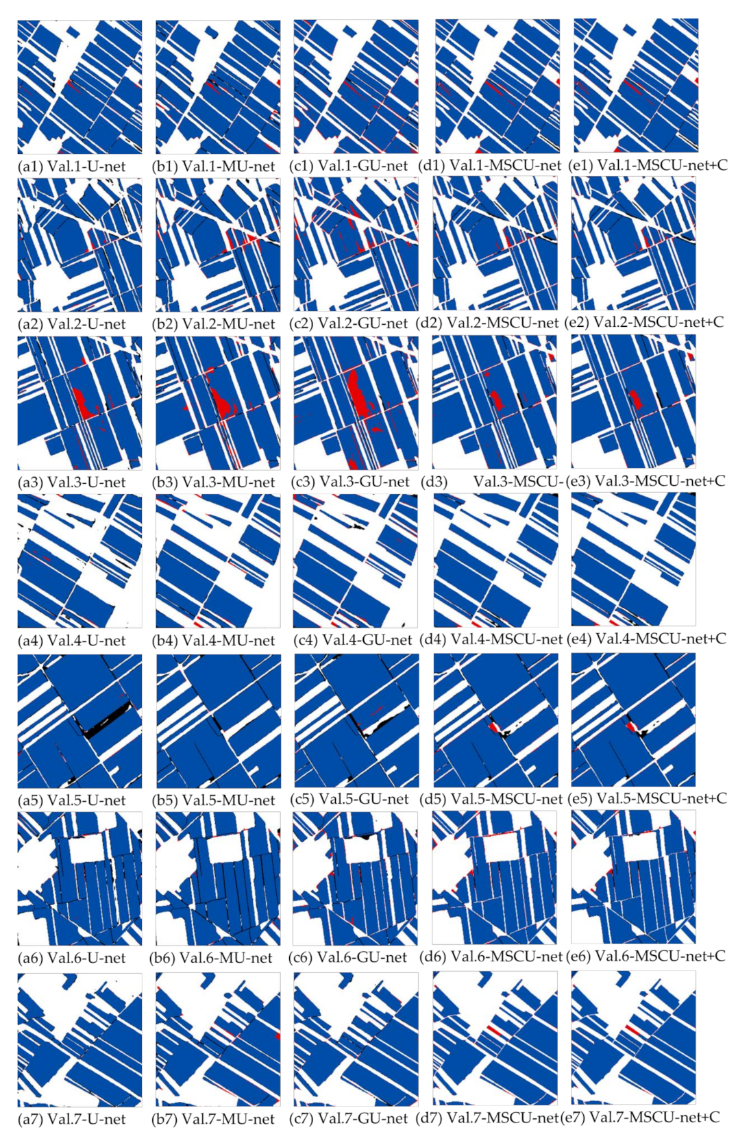
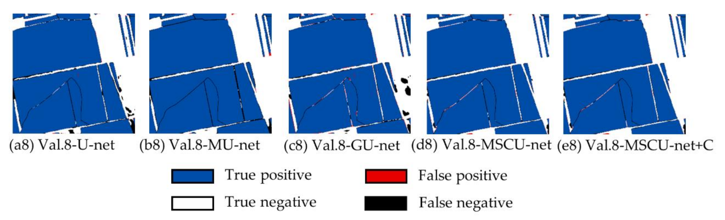
Firstly, the ablation experiments reveal that the developed MSCU-net+C has potential in mapping CRCA using Chinese high spatial resolution remote sensing images, and have improvements compared with the deep semantic segmentation networks, such as U-net, MU-net, GU-net and MSCU-net, and deep semantic segmentation networks. The attention mechanism is applied in the network as a form of image feature enhancement to improve the effectiveness of feature maps [42]. The experimental results show that the combination of attention mechanisms can capture feature information more sufficiently and achieve better performance [62]. The improvements used in this study lie in MSCG, the global loss function, CBAM, and FCCRF. The MSCU-net+C improves 0.0477/0.0394 in IOU_AVG/Kappa_AVG than U-net and get better classification performance. The MSCG can capture multiscale information and enrich the expression of feature maps [63], which results in a more thorough understanding of the input information. The global loss function is used to balance the network parameters of the high and low layers. Then, the CBAM can obtain better important information in the process of network learning CRCA. Lastly, the FCCRF is used to optimize classification results. The quantitative and qualitative accuracy assessment results revealed that the proposed MSCU-net+C is applicable to the CRCA classification.

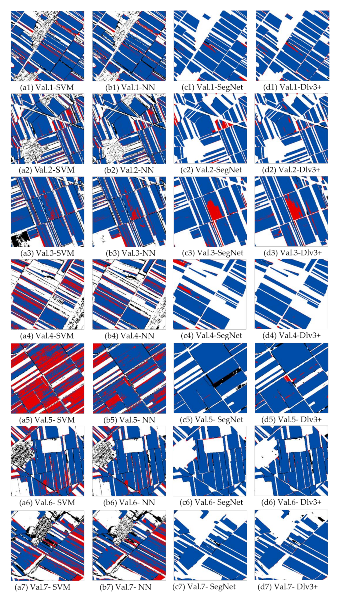
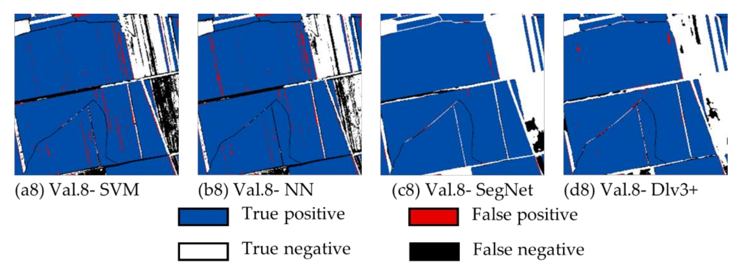
Secondly, the comparative experiment demonstrates that MSCU-net+C, SegNet, and Dlv3+ deep semantic segmentation methods alleviate edge information loss compared with SVM and NN traditional machine learning methods in extracting CRCA from high resolution remote sensing images. For traditional machine learning methods, most algorithms rely on the accuracy of the extracted features, including pixel values, shapes, textures, and positions, etc. However, deep semantic segmentation methods automatically can obtain high level relevant features directly from remote sensing images in CRCA classification, which reduces the work of designing feature extractors for each classification problem. In addition, the proposed MSCU-net+C method can capture contextual information and improve the effectiveness of feature information, which is the best method for classification performance in comparative experiments.

Finally, the CRCA classification results revealed that the deep semantic segmentation method can alleviate the salt-and-pepper problem effectively, which exists in the classification of high spatial resolution images commonly. Some studies adopt object-based approach to avoid the salt-and-pepper phenomenon in classification problems. However, the object-based classification depends on experience and knowledge to build the segmentation parameters, which is intend for strong subjectivity. Fortunately, the deep semantic segmentation method can preserve detailed edge information by performing both segmentation and pixel-based classification simultaneously. Thus, the deep semantic segmentation method is more suitable for identifying CRCA from high resolution multispectral remote sensing images.

Our proposed method can capture the border and details information of GF-1 B/D images for the CRCA mapping using encoder–decoder structure automatically. Thus, the prediction results of CRCA using GF-1 B/D performed well in this study. However, there are still some limitations worth noting. Firstly, more spectral information can be joined. The lignin and cellulose in crop residue are more sensitive with the spectrum of 1450–1960 nm and near 2100 nm [64]. The spectrum of the Chinese GF-5 image is ranging from visible bands to short wave infrared bands, and the GF-5 image can be combined with GF-1 B/D image to improve crop residue covered area mapping. Secondly, multitemporal remote sensing image features have the potential to improve the crop residue covered area classification results. The combination of multitemporal images can alleviate the interference of crops with similar spectral characteristics in the classification. Finally, the low imaging coverage of GF-1 B/D results in the limitation of application in regional areas. Recent studies of deep learning reveal that the trained model can be transferred into other data sources through transfer learning. Therefore, this study can be extended to other remote sensing images and other study areas for more crop residue cover mapping.

6. Conclusions

The developed MSCU-net+C deep semantic segmentation method can extract the deep features from the input image automatically through the code-encode structure, which is used to mapping CRCA by Chinese GF-1 B/D high spatial resolution image in this study. The quantitative evaluation of the ablation experiment and comparison experiment show that this proposed method has the best results, which can alleviate noise and identify CRCA that are scattered and irregular accurately.

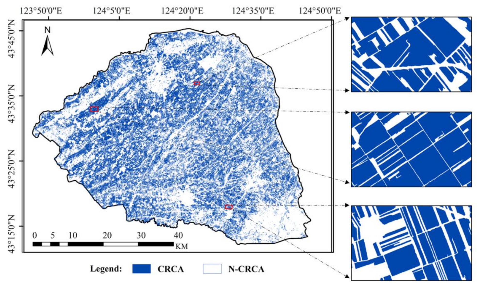
By comparing different models in the architecture ablation experiment, we found that the MSCG, the global loss function, and CBAM embed in the MSCU-net can significantly improve the network performance, especially the ability of feature maps information screening and feature expression. MSCU-net+C is constructed by combining FCCRF and MSCU-net, which can optimize the CRCA classification results further. It shows that the proposed method of MSCU-net+C is reasonable. By comparing different methods in model comparison, we found that deep semantic segmentation methods can get a higher classification accuracy and more detailed boundaries of CRCA than SVM and NN. Furthermore, we used the proposed method of MSCU-net+C to classify the CRCA in the whole study area.

The results provide evidence for the ability of MSCU-net+C to learn shape and contextual features, which reveal the effectiveness of this method for corn residue covered areas mapping. However, there are still three potential improvements and further applications in future research. (1) Multitemporal and multisource remote sensing data fusion may improve CRCA classification results further. (2) Owing to the representativeness of the study area and the generalization of the proposed model, the method can be applied to CRCA recognition in more regional areas through the transfer learning method in the North China Plain. (3) The spatial pattern and statistics result of CRCA can be used to support local government (i.e., practicing agricultural subsidies) and promote conservation tillage implementation.

References

1. Sorokin, A.; Owens, P.; Láng, V.; Jiang, Z.D.; Michéli, E.; Krasilnikov, P. “Black soils” in the Russian Soil Classification system, the US Soil Taxonomy and the WRB: Quantitative correlation and implications for pedodiversity assessment. CATENA 2021, 196, 104824. [Google Scholar] [CrossRef]
2. Liu, X.B.; Zhang, X.Y.; Wang, Y.X.; Sui, Y.Y.; Zhang, S.L.; Herbert, S.J.; Ding, G. Soil degradation: A problem threatening the sustainable development of agriculture in Northeast China. Plant Soil Environ. 2020, 56, 87–97. [Google Scholar] [CrossRef] [Green Version]
3. Hu, X.; Liu, J.; Wei, D.; Zhu, P.; Cui, X.A.; Zhou, B.; Wang, G. Effects of over 30-year of different fertilization regimes on fungal community compositions in the black soils of northeast China. Agric. Ecosyst. Environ. 2017, 248, 113–122. [Google Scholar] [CrossRef]
4. Bannari, A.; Staenz, K.; Champagne, C.; Khurshid, K.S. Spatial variability mapping of crop residue using Hyperion (EO-1) hyperspectral data. Remote Sens. 2015, 7, 8107–8127. [Google Scholar] [CrossRef] [Green Version]
5. Laflen, J.M.; Amemiya, M.; Hintz, E.A. Measuring crop residue cover. J. Soil Water Conserv. 1981, 36, 341–343. [Google Scholar]
6. Lahmar, R. Adoption of conservation agriculture in Europe: Lessons of the KASSA project. Land Use Policy 2010, 27, 4–10. [Google Scholar] [CrossRef]
7. Aase, J.K.; Tanaka, D.L. Reflectances from four wheat residue cover densities as influenced by three soil backgrounds. Agron. J. 1991, 83, 753–757. [Google Scholar] [CrossRef]
8. Zhang, M.Z.; Su, W.; Fu, Y.T.; Zhu, D.H.; Xue, J.H.; Huang, J.X.; Yao, C. Super-resolution enhancement of Sentinel-2 image for retrieving LAI and chlorophyll content of summer corn. Eur. J. Agron. 2019, 111, 125938. [Google Scholar] [CrossRef]
9. Su, W.; Zhang, M.Z.; Bian, D.H.; Liu, Z.; Huang, J.X.; Wang, W.; Wu, J.Y.; Guo, H. Phenotyping of corn plants using unmanned aerial vehicle (UAV) images. Remote Sens. 2019, 11, 2021. [Google Scholar] [CrossRef] [Green Version]
10. Quemada, M.; Daughtry, C.S.T. Spectral indices to improve crop residue cover estimation under varying moisture conditions. Remote Sens. 2016, 8, 660. [Google Scholar] [CrossRef] [Green Version]
11. Hamidisepehr, A.; Sama, M.P.; Turner, A.P.; Wendroth, O.O. A Method for Reflectance Index Wavelength Selection from Moisture-Controlled Soil and Crop Residue Samples. Trans. ASABE 2017, 60, 1479–1487. [Google Scholar] [CrossRef]
12. Omar, Z.; Stathaki, T. Hyperspectral unmixing overview: Geometrical, statistical, and sparse regression-based approaches. IEEE J. Sel. Top. Appl. Earth Obs. Remote Sens. 2012, 5, 354–379. [Google Scholar]
13. Mcnairn, H.; Protz, R. Mapping corn residue cover on agricultural fields in oxford county, ontario, using thematic mapper. Can. J. Remote Sens. 1993, 19, 152–159. [Google Scholar] [CrossRef]
14. Jin, X.; Ma, J.; Wen, Z.; Song, K. Estimation of maize residue cover using Landsat-8 OLI image spectral information and textural features. Remote Sens. 2015, 7, 14559–14575. [Google Scholar] [CrossRef] [Green Version]
15. Yue, J.; Tian, Q.; Dong, X.; Xu, K.; Zhou, C. Using hyperspectral crop residue angle index to estimate maize and winter-wheat residue cover: A laboratory study. Remote Sens. 2019, 11, 807. [Google Scholar] [CrossRef] [Green Version]
16. Wang, C.; Pan, X.; Liu, Y.; Li, Y.; Zhou, R.; Xie, X. Modeling the Effect of Moisture on the Reflectance of Crop Residues. Agron. J. 2012, 104, 1652–1657. [Google Scholar] [CrossRef]
17. Yue, J.; Tian, Q.; Tang, S.; Xu, K.; Zhou, C. A dynamic soil endmember spectrum selection approach for soil and crop residue linear spectral unmixing analysis. Int. J. Appl. Earth Obs. Geoinf. 2019, 78, 306–317. [Google Scholar] [CrossRef]
18. Khatami, R.; Mountrakis, G.; Stehman, S.V. A meta-analysis of remote sensing research on supervised pixel-based land-cover image classification processes: General guidelines for practitioners and future research. Remote Sens. Environ. 2016, 177, 89–100. [Google Scholar] [CrossRef] [Green Version]
19. Wood, E.M.; Pidgeon, A.M.; Radeloff, V.C.; Keuler, N.S. Image texture as a remotely sensed measure of vegetation structure. Remote Sens. Environ. 2012, 121, 516–526. [Google Scholar] [CrossRef]
20. Zhang, W.C.; Sun, X.; Fu, K.; Wang, C.Y.; Wang, H.Q. Object detection in high-resolution remote sensing images using rotation invariant parts based model. IEEE Geosci. Remote Sens. Lett. 2013, 11, 74–78. [Google Scholar] [CrossRef]
21. Clausi, D.A. An analysis of co-occurrence texture statistics as a function of grey level quantization. Can. J. Remote Sens. 2002, 28, 45–62. [Google Scholar] [CrossRef]
22. Pesaresi, M.; Benediktsson, J.A. A new approach for the morphological segmentation of high-resolution satellite imagery. IEEE Trans. Geosci. Remote Sens. 2001, 39, 309–320. [Google Scholar] [CrossRef] [Green Version]
23. Cheng, G.; Zhou, P.; Han, J. Learning rotation-invariant convolutional neural networks for object detection in VHR optical remote sensing images. IEEE Trans. Geosci. Remote Sens. 2016, 54, 7405–7415. [Google Scholar] [CrossRef]
24. Levinshtein, A.; Stere, A.; Kutulakos, K.N.; Fleet, D.J.; Dickinson, S.J.; Siddiqi, K. Turbopixels: Fast superpixels using geometric flows. IEEE Trans. Pattern Anal. Mach. Intell. 2009, 31, 2290–2297. [Google Scholar] [CrossRef] [Green Version]
25. Stutz, D.; Hermans, A.; Leibe, B. Superpixels: An evaluation of the state-of-the-art. Comput. Vis. Image Underst. 2018, 166, 1–27. [Google Scholar] [CrossRef] [Green Version]
26. Ciecholewski, M. Automated coronal hole segmentation from Solar EUV Images using the watershed transform. J. Vis. Commun. Image Represent. 2015, 33, 203–218. [Google Scholar] [CrossRef]
27. Cousty, J.; Bertrand, G.; Najman, L.; Couprie, M. Watershed cuts: Thinnings, shortest path forests, and topological watersheds. IEEE Trans. Pattern Anal. Mach. Intell. 2009, 32, 925–939. [Google Scholar] [CrossRef] [Green Version]
28. Balla-Arabé, S.; Gao, X. Geometric active curve for selective entropy optimization. Neurocomputing 2014, 139, 65–76. [Google Scholar] [CrossRef]
29. Ding, K.; Xiao, L.; Weng, G. Active contours driven by region-scalable fitting and optimized Laplacian of Gaussian energy for image segmentation. Signal Process. 2017, 134, 224–233. [Google Scholar] [CrossRef]
30. Wang, X.; Huang, J.; Feng, Q.; Yin, D. Winter Wheat Yield Prediction at County Level and Uncertainty Analysis in Main Wheat-producing Regions of China with Deep Learning Approaches. Remote Sens. 2020, 12, 1744. [Google Scholar] [CrossRef]
31. Huang, J.; Gómez-Dans, J.L.; Huang, H.; Ma, H.; Wu, Q.; Lewis, P.E.; Liang, S.; Chen, Z.; Xue, J.-H.; Wu, Y.; et al. Assimilation of remote sensing into crop growth models: Current status and perspectives. Agric. For. Meteorol. 2019, 276–277, 107609. [Google Scholar] [CrossRef]
32. Romero, A.; Gatta, C.; Camps-Valls, G. Unsupervised deep feature extraction for remote sensing image classification. IEEE Trans. Geosci. Remote Sens. 2016, 54, 1349–1362. [Google Scholar] [CrossRef] [Green Version]
33. Liu, S.; Ding, W.; Liu, C.; Liu, Y.; Wang, Y.; Li, H. ERN: Edge Loss Reinforced Semantic Segmentation Network for Remote Sensing Images. Remote Sens. 2018, 10, 1339. [Google Scholar] [CrossRef] [Green Version]
34. Kemker, R.; Salvaggio, C.; Kanan, C. Algorithms for semantic segmentation of multispectral remote sensing imagery using deep learning. ISPRS J. Photogramm. Remote Sens. 2018, 145, 60–77. [Google Scholar] [CrossRef] [Green Version]
35. Wang, J.; Sun, K.; Cheng, T.; Jiang, B.; Deng, C.; Zhao, Y.; Xiao, B. Deep high-resolution representation learning for visual recognition. IEEE Trans. Pattern Anal. Mach. Intell. 2020. [Google Scholar] [CrossRef] [Green Version]
36. Jung, Y.J.; Kim, M.J. Deeplab v3+ Based Automatic Diagnosis Model for Dental X-ray: Preliminary Study. J. Magn. 2020, 25, 632–638. [Google Scholar] [CrossRef]
37. Ronneberger, O.; Fischer, P.; Brox, T. U-net: Convolutional networks for biomedical image segmentation. In Proceedings of the International Conference on Medical Image Computing and Computer-Assisted Intervention, Munich, Germany, 5–9 October 2015; pp. 234–241. [Google Scholar]
38. Diakogiannis, F.I.; Waldner, F.; Caccetta, P.; Wu, C. Resunet-a: A deep learning framework for semantic segmentation of remotely sensed data. ISPRS J. Photogramm. Remote Sens. 2020, 162, 94–114. [Google Scholar] [CrossRef] [Green Version]
39. Zhou, Z.W.; Siddiquee, M.M.R.; Tajbakhsh, N.; Liang, J.M. Unet++: A nested u-net architecture for medical image segmentation. In Deep Learning in Medical Image Analysis and Multimodal Learning for Clinical Decision Support; Springer: Cham, Switzerland, 2018; pp. 3–11. [Google Scholar]
40. Woo, S.; Park, J.; Lee, J.Y.; Kweon, I.S. Cbam: Convolutional block attention module. In Proceedings of the European Conference on Computer Vision (ECCV), Munich, Germany, 8–14 September 2018; pp. 3–19. [Google Scholar]
41. Chen, L.; Tian, X.; Chai, G.; Zhang, X.; Chen, E. A New CBAM-P-Net Model for Few-Shot Forest Species Classification Using Airborne Hyperspectral Images. Remote Sens. 2021, 13, 1269. [Google Scholar] [CrossRef]
42. Chen, Z.; Fu, Y.; Zhang, Y.; Jiang, Y.G.; Xue, X.Y.; Sigal, L. Multi-level semantic feature augmentation for one-shot learning. IEEE Trans. Image Process. 2019, 28, 4594–4605. [Google Scholar] [CrossRef] [Green Version]
43. Thoma, D.P.; Gupta, S.C.; Bauer, M.E. Evaluation of optical remote sensing models for crop residue cover assessment. J. Soil Water Conserv. 2004, 59, 224–233. [Google Scholar]
44. Daughtry, C.S.; Doraiswamy, P.C.; Hunt, E.R., Jr.; Stern, A.J.; McMurtrey, J.E., III; Prueger, J.H. Remote sensing of crop residue cover and soil tillage intensity. Soil Tillage Res. 2006, 91, 101–108. [Google Scholar] [CrossRef]
45. Zhong, P.; Wang, R. Modeling and classifying hyperspectral imagery by CRFs with sparse higher order potentials. IEEE Trans. Geosci. Remote Sens. 2010, 49, 688–705. [Google Scholar] [CrossRef]
46. Zhang, P.; Ke, Y.; Zhang, Z.; Wang, M.; Li, P.; Zhang, S. Urban land use and land cover classification using novel deep learning models based on high spatial resolution satellite imagery. Sensors 2018, 18, 3717. [Google Scholar] [CrossRef] [PubMed] [Green Version]
47. Garg, L.; Shukla, P.; Singh, S.K.; Bajpai, V.; Yadav, U. Land Use Land Cover Classification from Satellite Imagery using mUnet: A Modified Unet Architecture. In Proceedings of the VISIGRAPP (4: VISAPP), Prague, Czech Republic, 25–27 February 2019; pp. 359–365. [Google Scholar]
48. Itti, L.; Koch, C.; Niebur, E. A model of saliency-based visual attention for rapid scene analysis. IEEE Trans. Pattern Anal. Mach. Intell. 1998, 20, 1254–1259. [Google Scholar] [CrossRef] [Green Version]
49. Larochelle, H.; Hinton, G.E. Learning to combine foveal glimpses with a third-order boltzmann machine. Adv. Neural Inf. Process. Syst. 2010, 23, 1243–1251. [Google Scholar]
50. Khan, A.; Sohail, A.; Zahoora, U.; Qureshi, A.S. A survey of the recent architectures of deep convolutional neural networks. Artif. Intell. Rev. 2020, 53, 5455–5516. [Google Scholar] [CrossRef] [Green Version]
51. Ioffe, S.; Szegedy, C. Batch normalization: Accelerating deep network training by reducing internal covariate shift. Int. Conf. Mach. Learn. 2015, 37, 448–456. [Google Scholar]
52. Buslaev, A.; Iglovikov, V.I.; Khvedchenya, E.; Parinov, A.; Druzhinin, M.; Kalinin, A.A. Albumentations: Fast and flexible image augmentations. Information 2020, 11, 125. [Google Scholar] [CrossRef] [Green Version]
53. Congalton, R.G. A review of assessing the accuracy of classifications of remotely sensed data. Remote Sens. Environ. 1991, 37, 35–46. [Google Scholar] [CrossRef]
54. Du, Z.R.; Yang, J.Y.; Ou, C.; Zhang, T.T. Smallholder crop area mapped with a semantic segmentation deep learning method. Remote Sens. 2019, 11, 888. [Google Scholar] [CrossRef] [Green Version]
55. Zheng, S.; Jayasumana, S.; Romera-Paredes, B.; Vineet, V.; Su, Z.Z.; Du, D.L.; Torr, P.H. Conditional random fields as recurrent neural networks. In Proceedings of the IEEE International Conference on Computer Vision, Santiago, Chile, 11–18 December 2015; pp. 1529–1537. [Google Scholar]
56. Cortes, C.; Vapnik, V. Support-vector networks. Mach. Learn. 1995, 20, 273–297. [Google Scholar] [CrossRef]
57. Maier, H.R.; Dandy, G.C. Neural networks for the prediction and forecasting of water resources variables: A review of modelling issues and applications. Environ. Model. Softw. 2000, 15, 101–124. [Google Scholar] [CrossRef]
58. Lin, T.; Xu, J.L.; Shen, X.Q.; Jiang, H.; Zhong, R.H.; Wu, S.S.; Ting, K.C. A spatiotemporal assessment of field residues of rice, maize, and wheat at provincial and county levels in China. GCB Bioenergy 2019, 11, 1146–1158. [Google Scholar] [CrossRef]
59. Gao, F.; Zhao, B.; Dong, S.T.; Liu, P.; Zhang, J.W. Response of maize root growth to residue management strategies. Agron. J. 2018, 110, 95–103. [Google Scholar] [CrossRef]
60. Shen, Y.; McLaughlin, N.; Zhang, X.P.; Xu, M.G.; Liang, A.Z. Effect of tillage and crop residue on soil temperature following planting for a Black soil in Northeast China. Sci. Rep. 2018, 8, 4500. [Google Scholar] [CrossRef] [Green Version]
61. Mupangwa, W.; Thierfelder, C.; Cheesman, S.; Nyagumbo, I.; Muoni, T.; Mhlanga, B.; Ngwira, A. Effects of maize residue and mineral nitrogen applications on maize yield in conservation-agriculture-based cropping systems of Southern Africa. Renew. Agric. Food Syst. 2020, 35, 322–335. [Google Scholar] [CrossRef]
62. Gao, T.Y.; Han, X.; Liu, Z.Y.; Sun, M.S. Hybrid attention-based prototypical networks for noisy few-shot relation classification. In Proceedings of the AAAI Conference on Artificial Intelligence, Honolulu, HI, USA, 27 January–1 February 2019; Volume 33, pp. 6407–6414. [Google Scholar]
63. Zhao, Q.H.; Xie, K.L.; Wang, G.H.; Li, Y. Land cover classification of polarimetric SAR with fully convolution network and conditional random field. Acta Geod. Cartogr. Sin. 2020, 49, 65–78. [Google Scholar]
64. Daughtry, C.S.T.; Hunt, E.R., Jr.; McMurtrey, J.E., III. Assessing crop residue cover using shortwave infrared reflectance. Remote Sens. Environ. 2004, 90, 126–134. [Google Scholar] [CrossRef]
Figure 1. The location of the study area (Lishu County) and covered GF-1 B/D image (Near-infrared: Band 4, Red: Band 3, Green: Band 2).
Remotesensing 13 02903 g001
Figure 2. Different corn residue covered areas from GF-1 B/D image in Lishu County (R1 is corn high stubble residue covered area, R2 is short-stubble residue covered area, R3 is non-CRCA).
Remotesensing 13 02903 g002
Figure 3. MSCU-net architecture. N1: Up-sampling of the image feature with a 2 × 2 window size; N2: Feature image fusion; N3: The repeated application of two 3 × 3 convolutions followed by batch normalization; N4: Max pooling with 2 × 2 window size for down-sampling; N5: Attention mechanism module; N6: Multiscale Convolution Group (MSCG); M: Loss function of the intermediate layer, E: Loss function of high layer.
Remotesensing 13 02903 g003
Figure 4. Channel attention module (CAM) and spatial attention module (SAM). P1: Maximum global pooling; P2: Global average pooling; P3: Maximum pooling of channels; P4: Average pooling of channels; MLP: Multilayer Perceptron; P5: The convolution kernel is 7 × 7 two-dimensional convolutions, followed by sigmoid activation function; P6: Element-wise addition; P7: Element-wise multiplication; P8: Channel merging.
Remotesensing 13 02903 g004
Figure 5. Multiscale Convolution Group (MSCG).
Remotesensing 13 02903 g005
Figure 6. The eight validation (Val) samples (Near-infrared: Band 4, Red: Band 3, Green: Band 2) and corresponding ground truth (GT) label.
Remotesensing 13 02903 g006
Figure 7. Classification results of ablation experiments using eight validation samples.
Remotesensing 13 02903 g007aRemotesensing 13 02903 g007b
Figure 8. Classification maps for SVM, NN, SegNet, and Dlv3+ on eight validation samples.
Remotesensing 13 02903 g008aRemotesensing 13 02903 g008b
Figure 9. The classification result of corn residue covered area using MSCU-net + C in Lishu county.
Remotesensing 13 02903 g009