
Using Machine Learning to Predict Retrofit Effects for a Commercial Building Portfolio


Abstract
:
1. Introduction
1.1. Motivation
1.2. Related Literature
1.2.1. The Applications of Data-Driven Methods in Existing Building Retrofit Studies
1.2.2. Advantage of Data-Driven Methods in Retrofit Savings Prediction
2. Database and Methodology
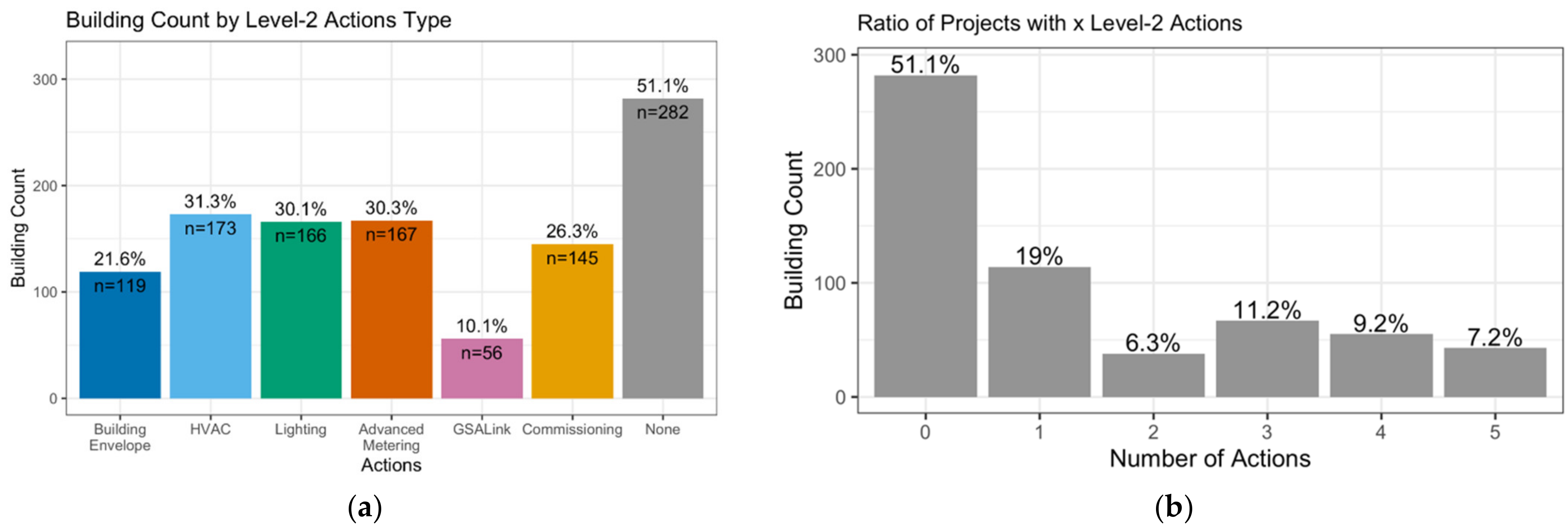
2.1. Data and Summary Statistics
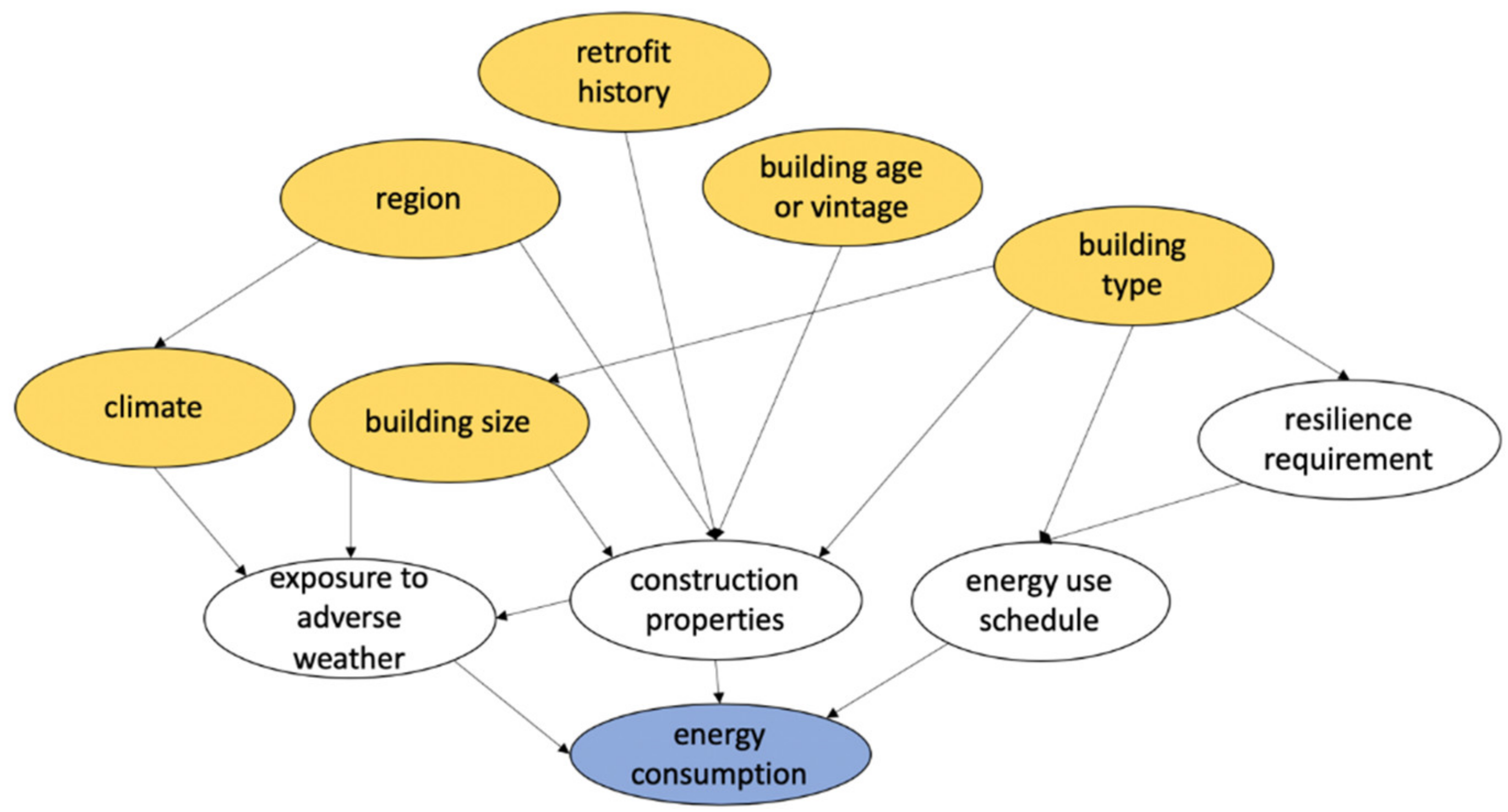
2.2. Assumptions and Confounding Variables
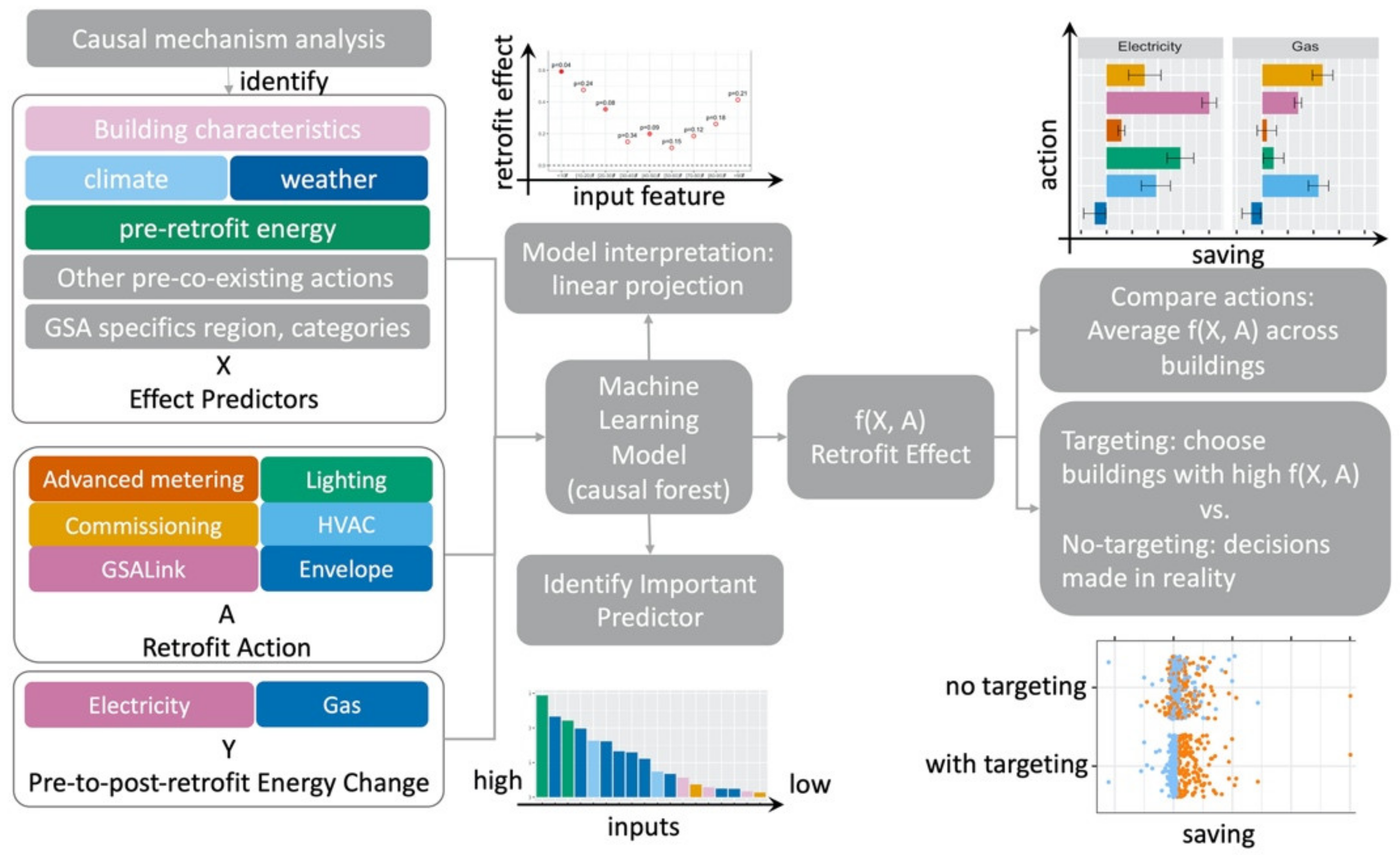
2.3. The Causal Forest Model
3. Results
3.1. The Average and Distribution of Retrofit Effect
3.2. Model Performance
3.3. The Benefit of Targeting Buildings with Higher Savings
3.4. The Association between Predicted Savings and Weather
4. Discussion
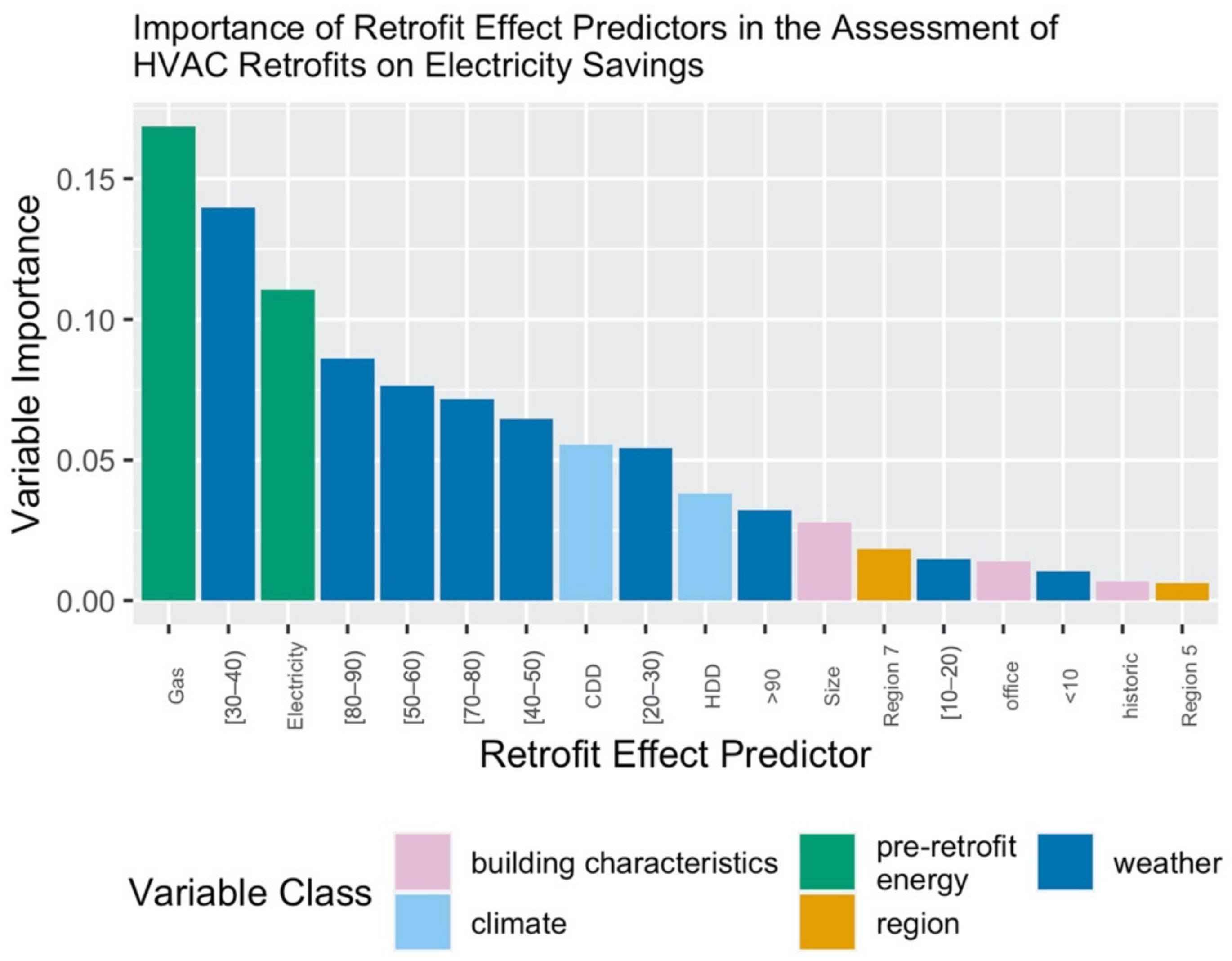
4.1. Variable Importance of Input Features
4.2. Results Comparison with Similar Studies
5. Conclusions
- The sample size is still rather small, given the desire to evaluate six classes of energy conservation actions (ECM) and 21 sets of sub-actions.
- The ECM action classifications are broad with limited or conflicting indications of the sub-actions taken.
- The retrofit records only have a completion date, not a start date, such that before and after data sets may not be accurately defined. In addition, many actions share the same completion date, which could lead to the contamination of “pre-retrofit” data with “during-retrofit” data, potentially resulting in biased savings estimates.
- As previously discussed, Executive Orders 13,423 and 13,693 are strong policy drivers for buildings in the GSA portfolio to reduce their energy consumption, whether they are retrofitted or not. This might make the retrofit savings estimates more conservative and the same action might reach higher savings in buildings without such a policy driver.
- Due to some un-documented retrofit actions, some retrofitted buildings might be categorized as un-retrofitted in the study. This could also lead to a more conservative savings estimation. In the future, such uncertainty should be reduced by improving the retrofit action documentation or including a sensitivity analysis.
- Even though co-existing or past actions are controlled for with indicator variables, the interactions between actions might be more complicated and not adequately accounted for.
- Acquire larger data sets with more thorough documentation of retrofit details and building characteristics and covering a larger variety of retrofit actions. With this improvement, savings could be predicted more accurately for a larger set of more specific actions.
- The decision support section is relatively simple in this study, as the focus is more on the savings prediction, rather than decision optimization. More complicated multi-objective optimization methods in Section 1.2.1 could be incorporated.
Author Contributions
Funding
Institutional Review Board Statement
Informed Consent Statement
Data Availability Statement
Acknowledgments
Conflicts of Interest
References
- U.S. Energy Information Administration (EIA), Annual Energy Review. 2019. Available online: https://www.eia.gov/totalenergy/data/annual/index.php (accessed on 27 December 2019).
- United States Environmental Protection Agency (EPA). US Energy Use Intensity by Property Type; Energy Star: Washington, DC, USA, 2018.
- Luddeni, G.; Krarti, M.; Pernigotto, G.; Gasparella, A. An analysis methodology for large-scale deep energy retrofits of existing building stocks: Case study of the Italian office building. Sustain. Cities Soc. 2018, 41, 296–311. [Google Scholar] [CrossRef]
- Zhai, J.; LeClaire, N.; Bendewald, M. Deep energy retrofit of commercial buildings: A key pathway toward low-carbon cities. Carbon Manag. 2011, 2, 425–430. [Google Scholar] [CrossRef]
- Zuhaib, S.; Goggins, J. Assessing evidence-based single-step and staged deep retrofit towards nearly zero-energy buildings (nZEB) using multi-objective optimisation. Energy Effic. 2019, 12, 1891–1920. [Google Scholar] [CrossRef]
- Granade, H.C.; Creyts, J.; Derkach, A.; Farese, P.; Nyquist, S.; Ostrowski, K. Unlocking Energy Efficiency in the US Economy; McKinsey Co. 2009. Available online: https://www.mckinsey.com/~/media/mckinsey/dotcom/client_service/epng/pdfs/unlocking%20energy%20efficiency/us_energy_efficiency_exc_summary.ashx (accessed on 22 October 2018).
- Brainerd, J.G.; Stobaugh, R.; Yergin, D.; Phillips, O. Energy Future: Report of the Energy Project at the Harvard Business School. Technol. Cult. 1981, 22, 217. [Google Scholar] [CrossRef]
- Fowlie, M.; Greenstone, M.; Wolfram, C. Do Energy Efficiency Investments Deliver? Evidence from the Weatherization Assistance Program. Q. J. Econ. 2018, 133, 1597–1644. [Google Scholar] [CrossRef] [Green Version]
- Liang, J.; Qiu, Y.; James, T.; Ruddell, B.; Dalrymple, M.; Earl, S.; Castelazo, A. Do energy retrofits work? Evidence from commercial and residential buildings in Phoenix. J. Environ. Econ. Manag. 2018, 92, 726–743. [Google Scholar] [CrossRef]
- Angrist, J.D.; Pischke, J.-S. Mastering’metrics: The Path from Cause to Effect; Princeton University Press: Princeton, NJ, USA, 2014. [Google Scholar]
- Allcott, H.; Greenstone, M. Measuring the Welfare Effects of Residential Energy Efficiency Programs; National Bureau of Economic Research: Cambridge, MA, USA, 2017. [Google Scholar]
- Zivin, J.G.; Novan, K. Upgrading Efficiency and Behavior: Electricity Savings from Residential Weatherization Programs. Energy J. 2016, 37, 1–24. [Google Scholar] [CrossRef]
- Dubin, J.A.; McFadden, D.L. A Heating and Cooling Load Model for Single-Family Detached Dwellings in Energy Survey Data; California Institute of Technology: Pasadena, CA, USA, 1983. [Google Scholar]
- Dubin, J.A.; Miedema, A.K.; Chandran, R.V. Price Effects of Energy-Efficient Technologies: A Study of Residential Demand for Heating and Cooling. RAND J. Econ. 1986, 17, 310. [Google Scholar] [CrossRef] [Green Version]
- Davis, L.W.; Fuchs, A.; Gertler, P. Cash for Coolers: Evaluating a Large-Scale Appliance Replacement Program in Mexico. Am. Econ. J. Econ. Policy 2014, 6, 207–238. [Google Scholar] [CrossRef] [Green Version]
- Scheer, J.; Clancy, M.; Hógáin, S.N. Quantification of energy savings from Ireland’s Home Energy Saving scheme: An ex post billing analysis. Energy Effic. 2012, 6, 35–48. [Google Scholar] [CrossRef]
- Grimes, A.; Preval, N.; Young, C.; Arnold, R.; Denne, T.; Howden-Chapman, P.; Telfar-Barnard, L. Does Retrofitted Insulation Reduce Household Energy Use? Theory and Practice. Energy J. 2016, 37, 165–186. [Google Scholar] [CrossRef]
- Burlig, F.; Knittel, C.; Rapson, D.; Reguant, M.; Wolfram, C. Machine Learning from Schools about Energy Efficiency. J. Assoc. Environ. Resour. Econ. 2020, 23908, 1181–1217. [Google Scholar] [CrossRef]
- Horn, T.D.M.; Borden, M. Cost Effectiveness; California Energy Commission: Sacramento, CA, USA, 1980. [Google Scholar]
- Levinson, A. How Much Energy Do Building Energy Codes Save? Evidence from California Houses. Am. Econ. Rev. 2016, 106, 2867–2894. [Google Scholar] [CrossRef] [Green Version]
- Blonz, J.A. The Welfare Costs of Misaligned Incentives: Energy Inefficiency and the Principal-Agent Problem. Financ. Econ. Discuss. Ser. 2019, 2019, 1–39. [Google Scholar] [CrossRef]
- Christensen, P.; Francisco, P.; Myers, E.; Souza, M. Decomposing the wedge between projected and realized returns in energy efficiency programs. E2e Work. Pap. 2020, 46, 1–37. [Google Scholar]
- Giraudet, L.-G.; Houde, S.; Maher, J.A. Moral Hazard and the Energy Efficiency Gap: Theory and Evidence. J. Assoc. Environ. Resour. Econ. 2018, 5, 755–790. [Google Scholar] [CrossRef] [Green Version]
- Allcott, H.; Greenstone, M. Is There an Energy Efficiency Gap? J. Econ. Perspect. 2012, 26, 3–28. [Google Scholar] [CrossRef]
- Xu, Y. Using Machine Learning to Target Retrofits in Commercial Buildings under Alternative Climate Change Scenarios; Carnegie Mellon University: Pittsburgh, PA, USA, 2020. [Google Scholar]
- ASHRAE. Ashrae Guideline 14-2014: Measurement of Energy, Demand and Water Savings. 2014. Available online: https://books.google.com/books?id=zlJkAQAACAAJ (accessed on 28 March 2018).
- Ma, Z.; Cooper, P.; Daly, D.; Ledo, L. Existing building retrofits: Methodology and state-of-the-art. Energy Build. 2012, 55, 889–902. [Google Scholar] [CrossRef]
- Grillone, B.; Danov, S.; Sumper, A.; Cipriano, J.; Mor, G. A review of deterministic and data-driven methods to quantify energy efficiency savings and to predict retrofitting scenarios in buildings. Renew. Sustain. Energy Rev. 2020, 131, 110027. [Google Scholar] [CrossRef]
- Efficiency Valuation Organisation. International Performance Measurement and Verification Protocol. Concepts and Options for Determining Energy and Water Savings; International Performance Measuremnt & Verification Protocol Committee: Golden, CO, USA, 2012. [Google Scholar]
- Marasco, D.E.; Kontokosta, C.E. Applications of machine learning methods to identifying and predicting building retrofit opportunities. Energy Build. 2016, 128, 431–441. [Google Scholar] [CrossRef] [Green Version]
- Salvalai, G.; Malighetti, L.E.; Luchini, L.; Girola, S. Analysis of different energy conservation strategies on existing school buildings in a Pre-Alpine Region. Energy Build. 2017, 145, 92–106. [Google Scholar] [CrossRef]
- Geyer, P.; Schlüter, A.; Cisar, S. Application of clustering for the development of retrofit strategies for large building stocks. Adv. Eng. Inform. 2017, 31, 32–47. [Google Scholar] [CrossRef]
- Knittel, C.; Stolper, S. Using Machine Learning to Target Treatment: The Case of Household Energy Use. Nat. Bur. Econ. Res. 2019, 26531, 1–47. [Google Scholar] [CrossRef]
- Allcott, H.; Kessler, J.B. The Welfare Effects of Nudges: A Case Study of Energy Use Social Comparisons. Am. Econ. J. 2015, 11, 236–276. [Google Scholar] [CrossRef]
- Reddy, T.A.; Saman, N.F.; Claridge, D.E.; Haberl, J.S.; Turner, H.W.D.; Chalifoux, A.T. Baselining Methodology for Facility-Level Monthly Energy Use-part 1: Theoretical aspects. ASHRAE Trans. 1997, 103, 336–347. [Google Scholar]
- Fels, M.F. PRISM: An introduction. Energy Build. 1986, 9, 5–18. [Google Scholar] [CrossRef]
- Reddy, T.A.; Claridge, D.; Wu, J. Statistical Modeling of Daily Energy Consumption in Commercial Buildings Using Multiple Regression and Principal Component Analysis. 1992. Available online: https://www.researchgate.net/publication/47612918_Statistical_Modeling_of_Daily_Energy_Consumption_in_Commercial_Buildings_Using_Multiple_Regression_and_Principal_Component_Analysis (accessed on 3 November 2016).
- Thamilseran, S.; Haberl, J.S. A Bin Method for Calculating Energy Conservation Retrofit Savings in Commercial Buildings. 1994. Available online: http://oaktrust.library.tamu.edu/handle/1969.1/6640 (accessed on 21 October 2016).
- Zhang, Y.; O’Neill, Z.; Dong, B.; Augenbroe, G. Comparisons of inverse modeling approaches for predicting building energy performance. Build. Environ. 2015, 86, 177–190. [Google Scholar] [CrossRef]
- Granderson, J.; Price, P. Evaluation of the Predictive Accuracy of Five Whole Building Baseline Models; LBNL-5886E; USDOE Office of Science (SC): Berkeley, CA, USA, 2012. [Google Scholar]
- Mackay, D.J.C. Bayesian Non-Linear Modeling for the Prediction Competition. In Maximum Entropy and Bayesian Methods; Springer Science and Business Media LLC: Berlin/Heidelberg, Germany, 1996; pp. 221–234. [Google Scholar]
- Brown, M.; Barrington-Leigh, C.; Brown, Z. Kernel regression for real-time building energy analysis. J. Build. Perform. Simul. 2012, 5, 263–276. [Google Scholar] [CrossRef]
- Mocanu, E.; Nguyen, P.; Gibescu, M.; Kling, W.L. Deep learning for estimating building energy consumption. Sustain. Energy Grids Netw. 2016, 6, 91–99. [Google Scholar] [CrossRef]
- Dong, B.; Cao, C.; Lee, S.E. Applying support vector machines to predict building energy consumption in tropical region. Energy Build. 2005, 37, 545–553. [Google Scholar] [CrossRef]
- Solomon, D.M.; Winter, R.L.; Boulanger, A.G.; Anderson, R.N.; Wu, L.L. Forecasting Energy Demand in Large Commercial Buildings Using Support Vector Machine Regression; Columbia University Libraries: New York, NY, USA, 2011. [Google Scholar]
- Heo, Y.; Zavala, V.M. Gaussian process modeling for measurement and verification of building energy savings. Energy Build. 2012, 53, 7–18. [Google Scholar] [CrossRef]
- Yu, Z.; Haghighat, F.; Fung, B.C.M.; Yoshino, H. A decision tree method for building energy demand modeling. Energy Build. 2010, 42, 1637–1646. [Google Scholar] [CrossRef] [Green Version]
- Behl, M.; Mangharam, R. Evaluation of DR-Advisor on the ASHRAE Great Energy Predictor Shootout Challenge. 2014. Available online: http://repository.upenn.edu/cgi/viewcontent.cgi?article=1093&context=mlab_papers (accessed on 16 May 2017).
- Asadi, E.; da Silva, M.C.G.; Antunes, C.H.; Dias, L.; Glicksman, L. Multi-objective optimization for building retrofit: A model using genetic algorithm and artificial neural network and an application. Energy Build. 2014, 81, 444–456. [Google Scholar] [CrossRef]
- Ascione, F.; Bianco, N.; De Masi, R.F.; De Stasio, C.; Mauro, G.M.; Vanoli, G.P. Multi-objective optimization of the renewable energy mix for a building. Appl. Therm. Eng. 2016, 101, 612–621. [Google Scholar] [CrossRef]
- Ascione, F.; Bianco, N.; Mauro, G.M.; Napolitano, D.F.; Vanoli, G.P. A Multi-Criteria Approach to Achieve Constrained Cost-Optimal Energy Retrofits of Buildings by Mitigating Climate Change and Urban Overheating. Climate 2018, 6, 37. [Google Scholar] [CrossRef] [Green Version]
- Bichiou, Y.; Krarti, M. Optimization of envelope and HVAC systems selection for residential buildings. Energy Build. 2011, 43, 3373–3382. [Google Scholar] [CrossRef]
- Deb, K.; Pratap, A.; Agarwal, S.; Meyarivan, T. A fast and elitist multiobjective genetic algorithm: NSGA-II. IEEE Trans. Evol. Comput. 2002, 6, 182–197. [Google Scholar] [CrossRef] [Green Version]
- Delgarm, N.; Sajadi, B.; Delgarm, S.; Kowsary, F. A novel approach for the simulation-based optimization of the buildings energy consumption using NSGA-II: Case study in Iran. Energy Build. 2016, 127, 552–560. [Google Scholar] [CrossRef]
- Magnier, L.; Haghighat, F. Multiobjective optimization of building design using TRNSYS simulations, genetic algorithm, and Artificial Neural Network. Build. Environ. 2010, 45, 739–746. [Google Scholar] [CrossRef]
- Ascione, F.; Bianco, N.; De Stasio, C.; Mauro, G.M.; Vanoli, G.P. Artificial neural networks to predict energy performance and retrofit scenarios for any member of a building category: A novel approach. Energy 2017, 118, 999–1017. [Google Scholar] [CrossRef]
- Siddharth, V.; Ramakrishna, P.; Geetha, T.; Sivasubramaniam, A. Automatic generation of energy conservation measures in buildings using genetic algorithms. Energy Build. 2011, 43, 2718–2726. [Google Scholar] [CrossRef]
- Lara, R.A.; Pernigotto, G.; Cappelletti, F.; Romagnoni, P.; Gasparella, A. Energy audit of schools by means of cluster analysis. Energy Build. 2015, 95, 160–171. [Google Scholar] [CrossRef]
- Lee, S.H.; Hong, T.; Piette, M.A.; Taylor-Lange, S.C. Energy retrofit analysis toolkits for commercial buildings: A review. Energy 2015, 89, 1087–1100. [Google Scholar] [CrossRef] [Green Version]
- Burrell, M. GSA Looks Back at the American Recovery and Reinvestment Act. 2016. Available online: https://www.gsa.gov/blog/2016/02/18/gsa-looks-back-at-the-american-recovery-and-reinvestment-act (accessed on 12 July 2020).
- FedCenter. EO 13693 (Archive)—Revoked by EO 13834 on 17 May 2018, Sec 8. 2019. Available online: https://www.fedcenter.gov/programs/eo13693/ (accessed on 12 July 2020).
- Wenninger, S. Advanced Metering Ensures Cost Effective and Efficient Federal Facilities. 2013. Available online: https://www.gsa.gov/blog/2013/01/22/Advanced-Metering-Ensures-Cost-Effective-and-Efficient-Federal-Facilities (accessed on 2 January 2020).
- GSA Public Buildings Service. The Building Commissioning Guide. 2015. Available online: https://www.gsa.gov/cdnstatic/BCG_3_30_Final_R2-x221_0Z5RDZ-i34K-pR.pdf (accessed on 16 April 2020).
- GSA. Lighting. 2018. Available online: https://www.gsa.gov/governmentwide-initiatives/sustainability/emerging-building-technologies/gsa-technology-deployment-maps/lighting (accessed on 12 September 2018).
- Kontokosta, C.E. Modeling the energy retrofit decision in commercial office buildings. Energy Build. 2016, 131, 1–20. [Google Scholar] [CrossRef]
- Deschênes, O.; Greenstone, M. Climate Change, Mortality, and Adaptation: Evidence from Annual Fluctuations in Weather in the US. Am. Econ. J. Appl. Econ. 2007, 3, 152–185. [Google Scholar] [CrossRef]
- Dell, M.; Jones, B.; Olken, B. What Do We Learn from the Weather? The New Climate-Economy Literature. J. Econ Lit. 2013, 52, 740–798. [Google Scholar] [CrossRef] [Green Version]
- Auffhammer, M.; Mansur, E.T. Measuring climatic impacts on energy consumption: A review of the empirical literature. Energy Econ. 2014, 46, 522–530. [Google Scholar] [CrossRef] [Green Version]
- Wager, S.; Athey, S. Estimation and Inference of Heterogeneous Treatment Effects using Random Forests. J. Am. Stat. Assoc. 2018, 113, 1228–1242. [Google Scholar] [CrossRef] [Green Version]
- Tibshirani, J.; Athey, S.; Wager, S. Generalized Random Forests. 2020. Available online: https://CRAN.R-project.org/package=grf (accessed on 29 June 2021).
- Mills, E.; Friedman, H.; Powell, T.; Bourassa, N.; Claridge, D.; Piette, M.A. The Cost-Effectiveness of Commercial-Buildings Commissioning; Berkeley Lab: Berkeley, CA, USA, 2004; p. 98. [Google Scholar]
- Chidiac, S.; Catania, E.; Morofsky, E.; Foo, S. Effectiveness of single and multiple energy retrofit measures on the energy consumption of office buildings. Energy 2011, 36, 5037–5052. [Google Scholar] [CrossRef]
- Faruqui, A.; Arritt, K.; Sergici, S. The impact of advanced metering infrastructure on energy conservation: A case study of two utilities. Electr. J. 2017, 30, 56–63. [Google Scholar] [CrossRef]
- Paschmann, M.H.; Paulus, S. The Impact of Advanced Metering Infrastructure on Residential Electricity Consumption: Evidence from California. EWI Working Paper No. 17/08. 2017. Available online: https://www.econstor.eu/handle/10419/172838 (accessed on 29 June 2021).
- Lin, G.; Kramer, H.; Granderson, J. Building fault detection and diagnostics: Achieved savings, and methods to evaluate algorithm performance. Build. Environ. 2020, 168, 106505. [Google Scholar] [CrossRef] [Green Version]
- Carli, R.; Dotoli, M.; Pellegrino, R.; Ranieri, L. Using multi-objective optimization for the integrated energy efficiency improvement of a smart city public buildings’ portfolio. In Proceedings of the 2015 IEEE International Conference on Automation Science and Engineering (CASE), Gothenburg, Sweden, 24–28 August 2015; Institute of Electrical and Electronics Engineers (IEEE): New York, NY, USA, 2015; pp. 21–26. [Google Scholar]
- Diakaki, C.; Grigoroudis, E.; Kabelis, N.; Kolokotsa, D.; Kalaitzakis, K.; Stavrakakis, G. A multi-objective decision model for the improvement of energy efficiency in buildings. Energy 2010, 35, 5483–5496. [Google Scholar] [CrossRef]
- Lok, J.; Gill, R.; Van Der Vaart, A.; Robins, J. Estimating the causal effect of a time-varying treatment on time-to-event using structural nested failure time models. Stat. Neerlandica 2004, 58, 271–295. [Google Scholar] [CrossRef]
- Hernán, M.A.; Brumback, B.; Robins, J.M. Marginal Structural Models to Estimate the Joint Causal Effect of Nonrandomized Treatments. J. Am. Stat. Assoc. 2001, 96, 440–448. [Google Scholar] [CrossRef]
- Robins, J.M. The analysis of randomized and non-randomized AIDS treatment trials using a new approach to causal inference in longitudinal studies. In Health Service Research Methodology: A Focus on AIDS; National Center for Health Service Research: Washington, DC, USA, 1989; pp. 113–159. [Google Scholar]


| Engineering Model or Projection | Empirical Approach | n | Realization Rate 1 | Building Use | References |
|---|---|---|---|---|---|
| NEAT | Experimental (RED) | around 30,000 | 30% in total energy | Residential | [8] |
| TREAT | DD, event study | 101,881 | 35% in total energy 58% in energy expenses | Residential | [11] |
| DEER | DD, IV | 275 | 79% in electricity for AC homes 0% in electricity for non-AC homes | Residential | [12] |
| [13] | Experimental + engineering 2 | 504 | 87% in cooling 88–92% in heating | Residential | [14] |
| World Bank | DD, event study, matching | 1,162,775 | About 25% in electricity reduction from fridge replacement | Residential | [15] |
| Dwelling Energy Assessment Procedure (DEAP) | DD | 640,000 | 64 ± 8% | Residential | [16] |
| Net Benefit Model | DD | 12,000 | 1/3 | Residential | [17] |
| Not specified | Time-series approach | 2094 | 24% overall, 49% for HVAC, 42% for lighting | K-12 school | [18] |
| Not specified | DD | 847 | 30–50% | Commercial and residential | [9] |
| [19] | Repeated cross-sectional comparison controlling for observables | Around 7000 | <32% 3 | Residential | [20] |
| Role of the Model | Model | Source |
|---|---|---|
| M&V inverse modeling | Linear regression | [35,36,37,38] |
| Piecewise linear regression | [35,39,40] | |
| Neural network (shallow) | [39,41,42] | |
| Deep learning | [43] | |
| Support vector machine regression (SVR) | [44,45] | |
| Kernel regression | [42] | |
| Gaussian process regression | [39,46] | |
| Gaussian mixture regression | [39] | |
| Decision tree | [47] | |
| Random forest | [48] | |
| Multi-objective optimization | Genetic algorithm (GA) | [49,50,51,52] |
| Nondominated sorting genetic algorithm II (NSGA-II) | [53,54,55] | |
| Particle swarm optimization | [52] | |
| Sequential search | [52] | |
| Predict retrofit decisions | Falling rule list | [30] |
| Approximate BES results | Neural network (shallow) | [49,55,56] |
| Generate inputs for BES parametric runs | Genetic algorithm (GA) | [57] |
| Identify representative buildings | Clustering | [31,58] |
| Estimate retrofit effect | Elastic nets | [34] |
| Gradient forest | [34] | |
| Causal forest | [33] |
| Retrofit Effect Predictor | Min | Mean | Median | Max | St. Dev. | |
|---|---|---|---|---|---|---|
| withre trofit | Electricity (kBtu/sqft/year) | 1.85 | 41.67 | 38.72 | 287.25 | 20.89 |
| Gas (kBtu/sqft/year) | 0.01 | 21.96 | 21.14 | 132.22 | 17.80 | |
| Cooling degree day (CDD) | 58.6 | 1409.3 | 1160.2 | 4628.2 | 989.5 | |
| Heating degree day (HDD) | 71.5 | 4484.1 | 4667.1 | 9172.7 | 2005.2 | |
| Gross square footage | 5912 | 402,742 | 269,946 | 3993,881 | 456,913 | |
| without retrofit | Electricity (kBtu/sqft/year) | 2.11 | 45.21 | 40.21 | 182.01 | 23.93 |
| Gas (kBtu/sqft/year) | 0.00 | 29.94 | 21.07 | 283.68 | 30.77 | |
| Cooling degree day (CDD) | 20.9 | 1398.5 | 1363.7 | 4589.0 | 961.2 | |
| Heating degree day (HDD) | 184.3 | 4460.4 | 4188.3 | 10,580.2 | 2389.8 | |
| Gross square footage | 1161 | 216,610 | 65,055 | 3456,919 | 428,105 |
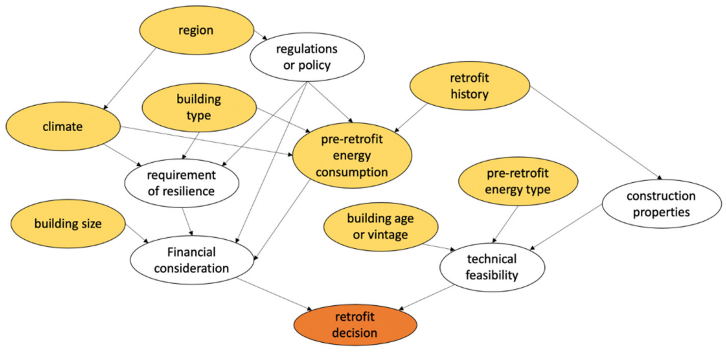
| Retrofit Effect Predictor Class | Retrofit Effect Predictor |
|---|---|
| Building characteristics | Building size in gross square footage. |
| Whether a building is a historic building. | |
| Whether a building had a LEED certificate before the retrofit project | |
| Whether a building is an office building or a courthouse | |
| Weather (average annual number of days with daily mean temperature within a certain range) | A total of 8 variables, the kth variable indicating the annual average number of days with daily temperature in the kth temperature bin. The temperature bins are below 10 °F, between 10 °F and 20 °F, …, between 80 and 90 °F, and above 90 °F. The 60 °F to 70 °F bin is left out as a reference. |
| Climate | 1981–2010 climate normal of annual cooling degree day (CDD), and annual heating degree day (HDD) |
| Pre-retrofit energy | Average monthly electricity, natural gas, chilled water, and steam consumption in kBtu/sqft/year. |
| Region | A total of 10 indicator variables, the kth indicator variable representing whether a building is in GSA region k. Region 1 is left out as the reference level. |
| Category | A total of 3 indicator variables, each corresponding to a GSA building category designation of B, E, or I. Category A is left out as the reference level 1. |
| Previous actions | Indicator variables of pre- or co-existing action categories. |
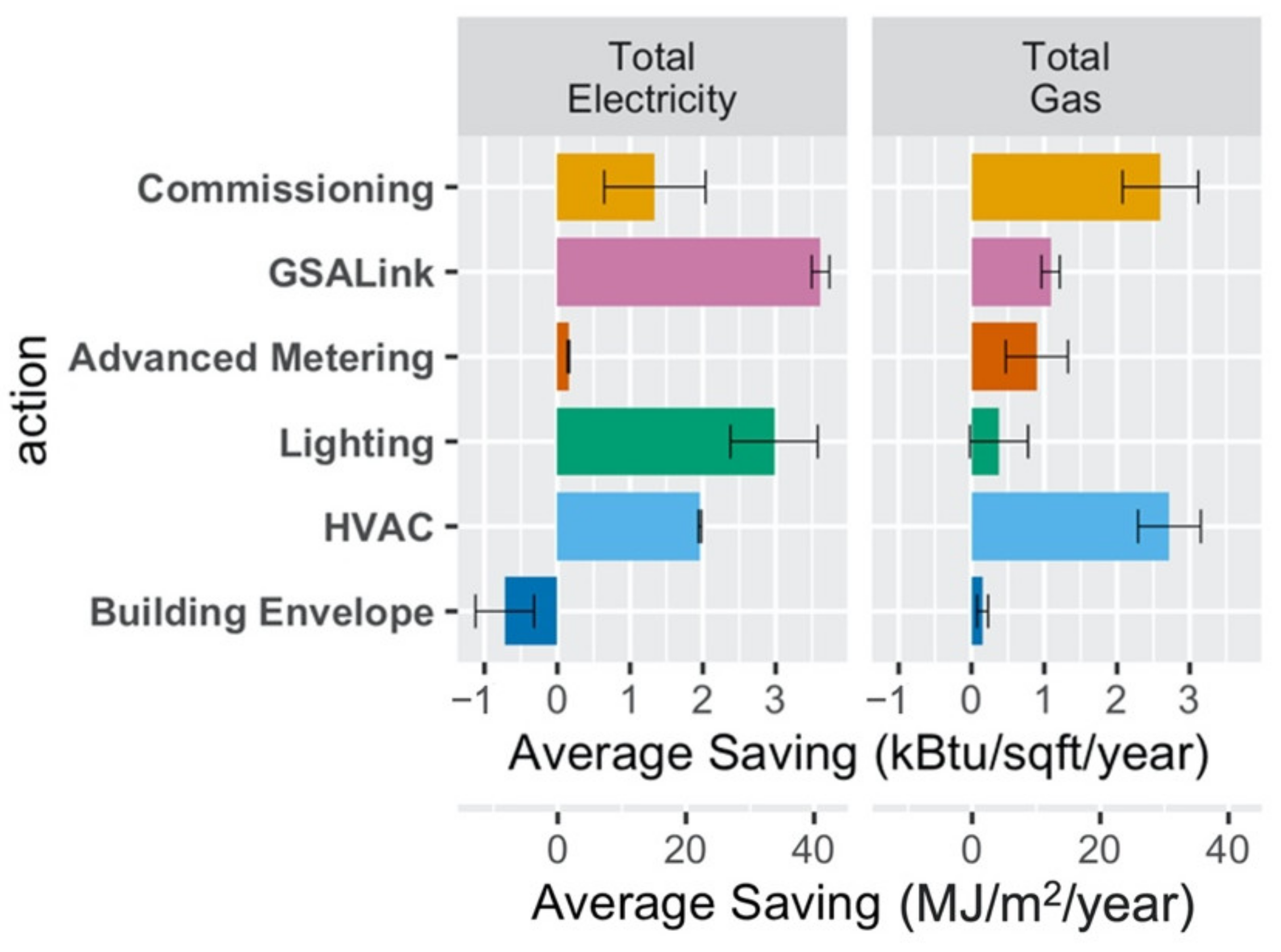
| Fuel | Action Type | Action | Summary Statistics | |||||
|---|---|---|---|---|---|---|---|---|
| Min | Q1 | Median | Q3 | Max | Mean | |||
| Electricity | Capital | Building envelope | −5.09 | −2.84 | −0.82 | 1.58 | 4.47 | −0.66 |
| HVAC | −5.02 | −1.86 | 1.53 | 4.76 | 11.71 | 1.90 | ||
| Lighting | −4.36 | 0.52 | 2.20 | 4.53 | 14.20 | 2.55 | ||
| Operational | Advanced metering | −1.41 | −0.09 | 0.36 | 0.93 | 2.86 | 0.47 | |
| Commissioning | −7.15 | −2.75 | 1.56 | 3.57 | 11.00 | 0.94 | ||
| GSALink | 1.04 | 3.40 | 4.26 | 5.57 | 10.60 | 4.87 | ||
| Gas | Capital | Building envelope | −4.81 | −2.47 | −1.10 | 0.97 | 1.95 | −0.89 |
| HVAC | −1.93 | 1.04 | 2.75 | 3.83 | 8.50 | 2.55 | ||
| Lighting | −4.30 | −1.15 | 0.06 | 1.61 | 6.78 | 0.35 | ||
| Operational | Advanced metering | −3.63 | −1.15 | −0.24 | 1.51 | 6.86 | 0.49 | |
| Commissioning | −1.24 | 0.88 | 1.97 | 3.76 | 8.56 | 2.62 | ||
| GSALink | 0.41 | 0.69 | 0.89 | 1.24 | 1.81 | 0.98 | ||
| Retrofit Action | The Absolute Value of the Mean Forest Prediction Score—1 | The p-Value of the Differential Forest Prediction Score | ||
|---|---|---|---|---|
| Electricity | Gas | Electricity | Gas | |
| Advanced metering | 1.78 | 0.87 | 0.94 | 0.04 * |
| Building envelope | 0.37 | 0.13 | 0.07 | 0.49 |
| Commissioning | 0.98 | 0.15 | 0.04 * | 0.34 |
| GSALink | 0.19 | 1.55 | 0.95 | 0.93 |
| HVAC | 0.45 | 0.01 | 0.00 *** | 0.27 |
| Lighting | 0.13 | 1.41 | 0.21 | 0.73 |
Publisher’s Note: MDPI stays neutral with regard to jurisdictional claims in published maps and institutional affiliations. |
© 2021 by the authors. Licensee MDPI, Basel, Switzerland. This article is an open access article distributed under the terms and conditions of the Creative Commons Attribution (CC BY) license (https://creativecommons.org/licenses/by/4.0/).
Share and Cite
Xu, Y.; Loftness, V.; Severnini, E. Using Machine Learning to Predict Retrofit Effects for a Commercial Building Portfolio. Energies 2021, 14, 4334. https://doi.org/10.3390/en14144334
Xu Y, Loftness V, Severnini E. Using Machine Learning to Predict Retrofit Effects for a Commercial Building Portfolio. Energies. 2021; 14(14):4334. https://doi.org/10.3390/en14144334
Chicago/Turabian StyleXu, Yujie, Vivian Loftness, and Edson Severnini. 2021. "Using Machine Learning to Predict Retrofit Effects for a Commercial Building Portfolio" Energies 14, no. 14: 4334. https://doi.org/10.3390/en14144334
APA StyleXu, Y., Loftness, V., & Severnini, E. (2021). Using Machine Learning to Predict Retrofit Effects for a Commercial Building Portfolio. Energies, 14(14), 4334. https://doi.org/10.3390/en14144334