
Multi-Year Simulation of Western Lake Erie Hydrodynamics and Biogeochemistry to Evaluate Nutrient Management Scenarios


Abstract
:1. Introduction
2. Methods
2.1. Study Site and Field Data
2.2. Model Description
2.3. Initial and Boundary Conditions
2.4. Model Calibration
2.5. Phosphorus Loading Reduction Scenarios
3. Results
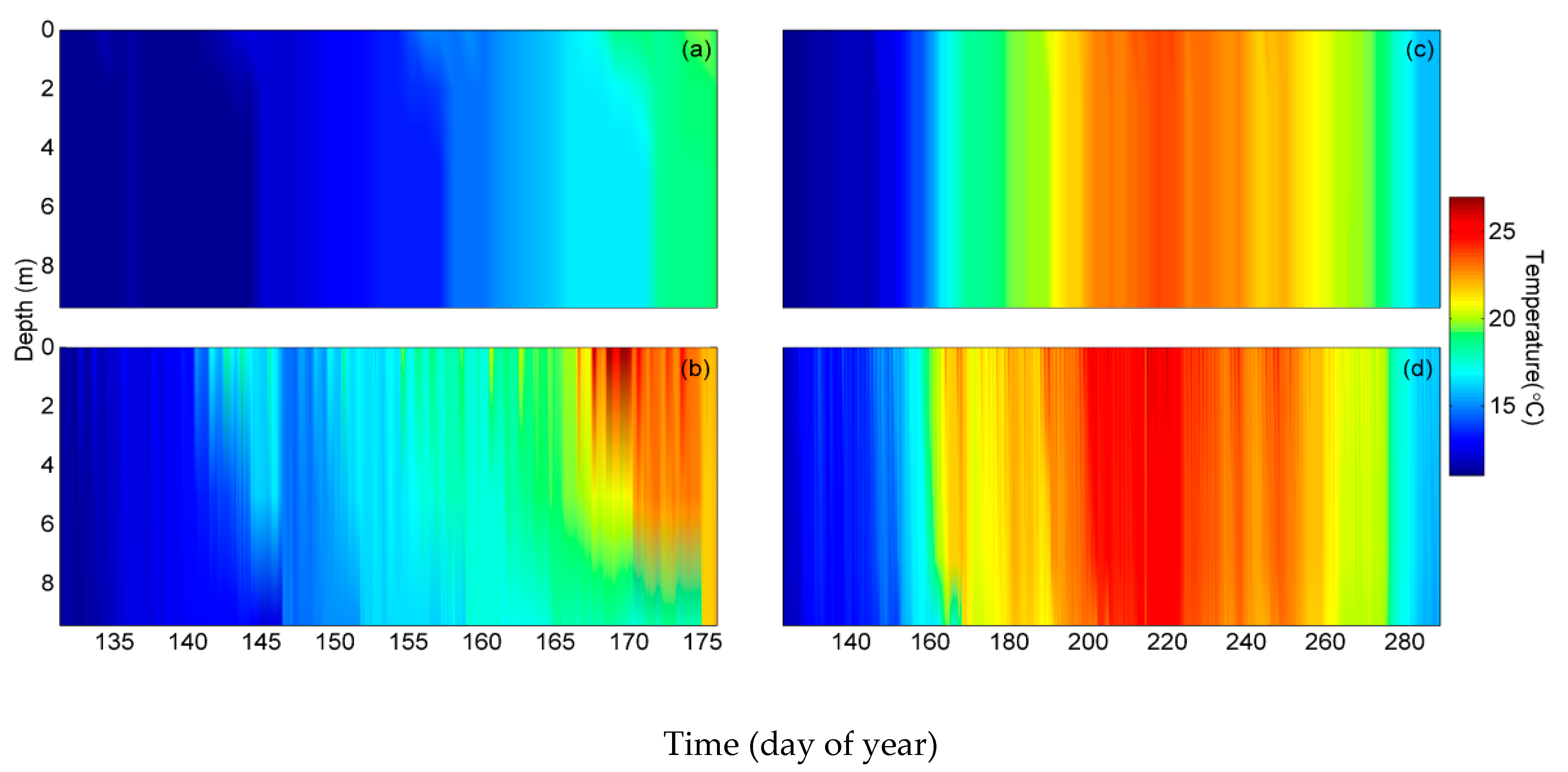
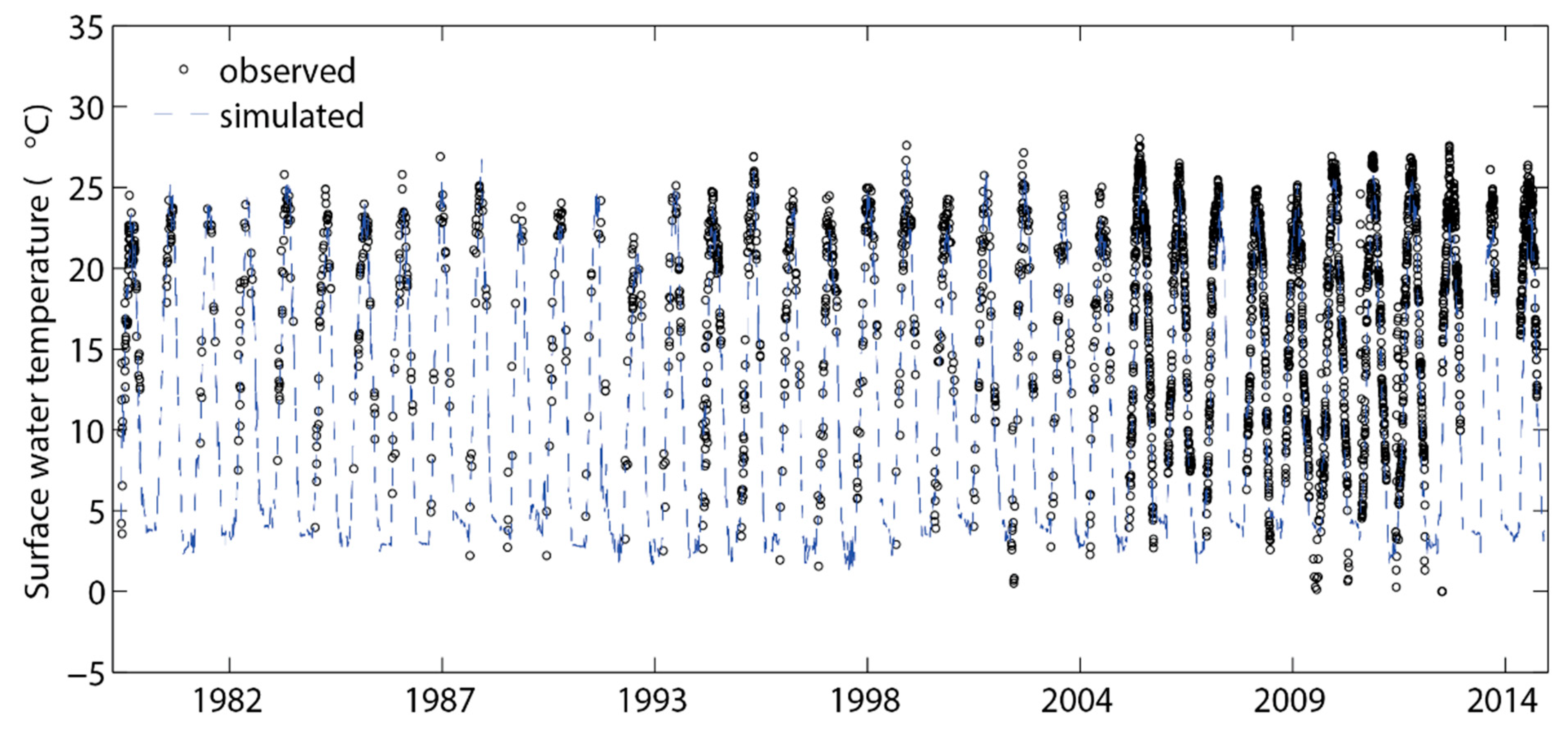
3.1. Temperature, Water Levels, and Ice Cover
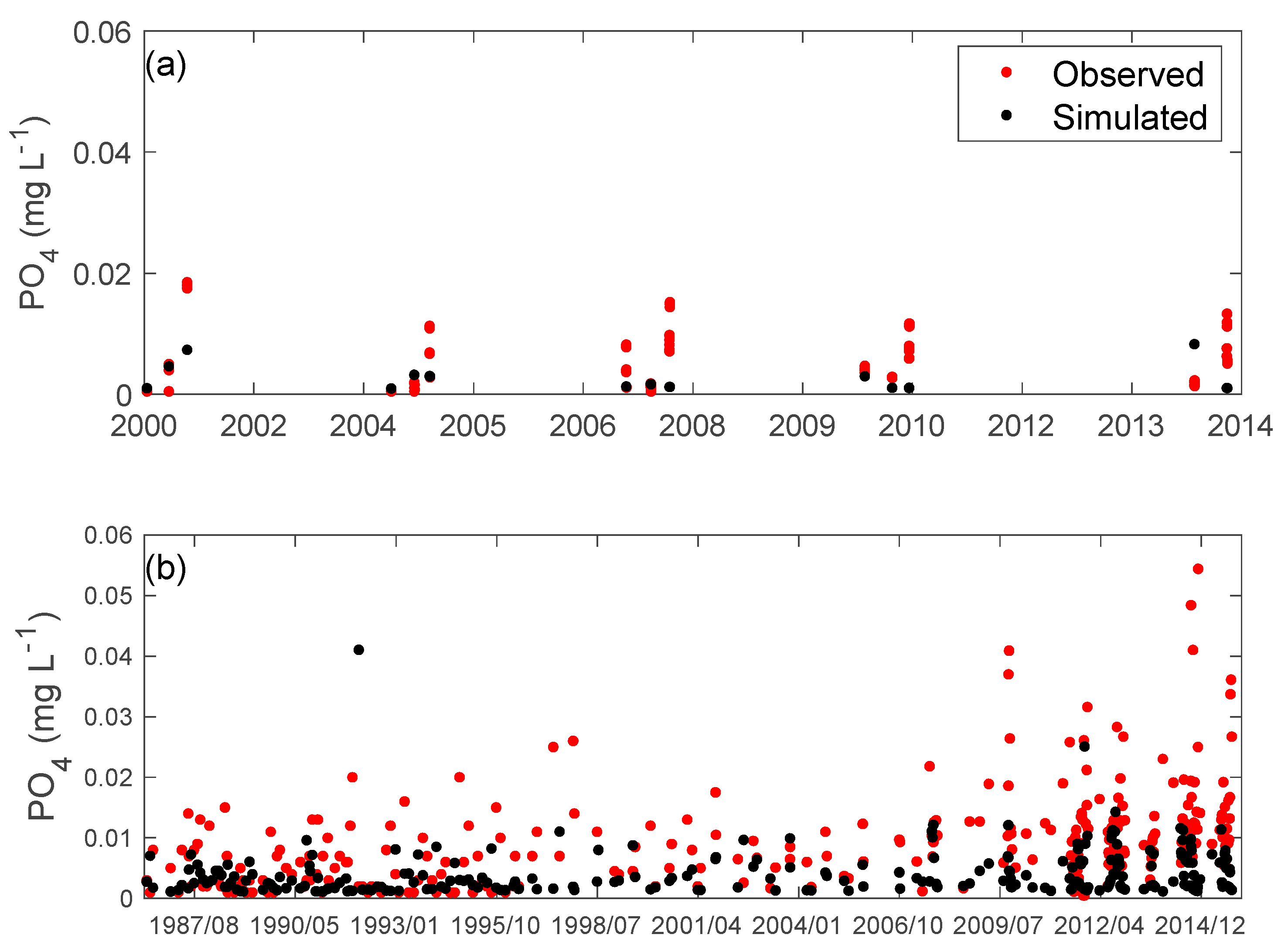
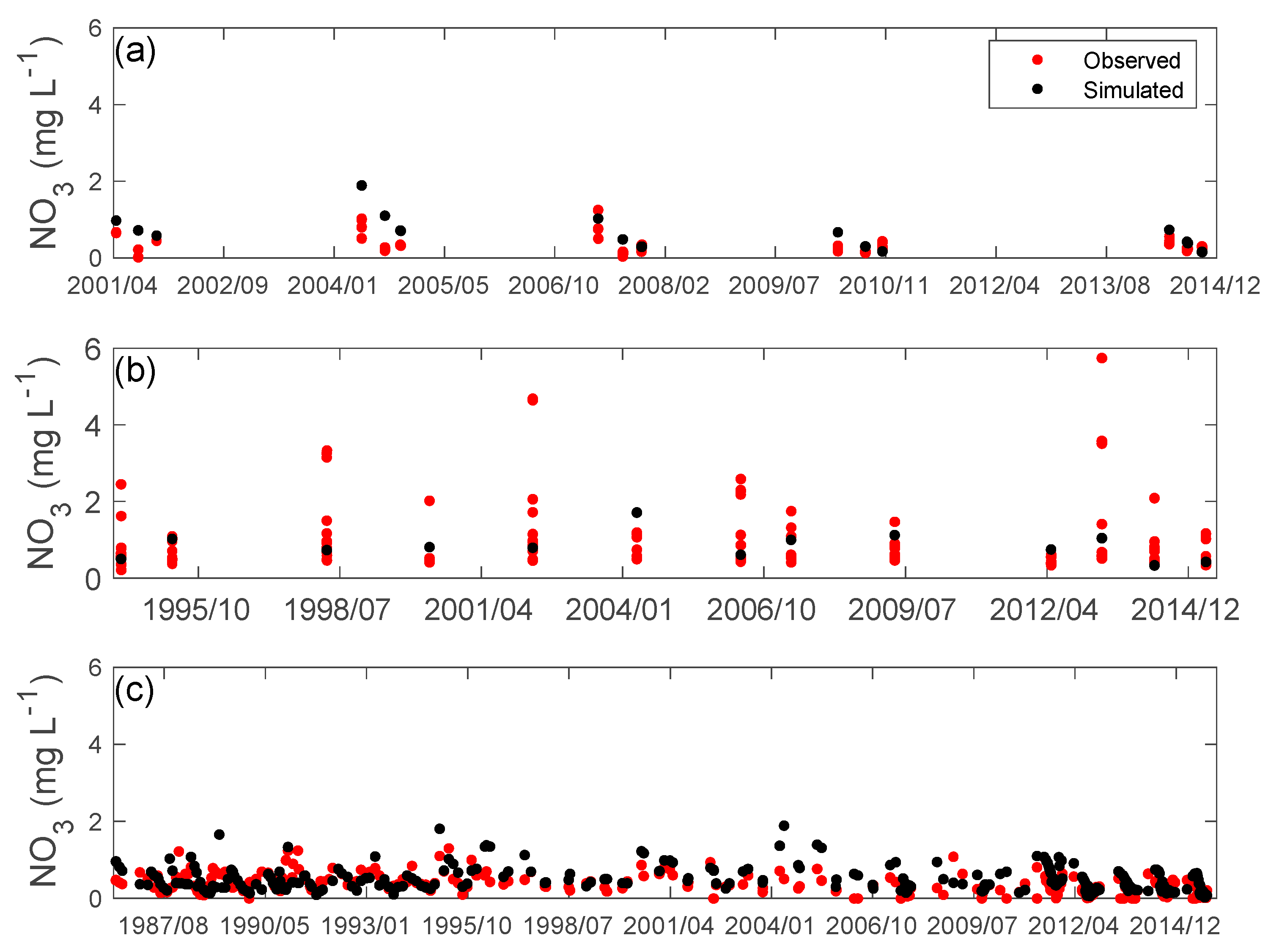
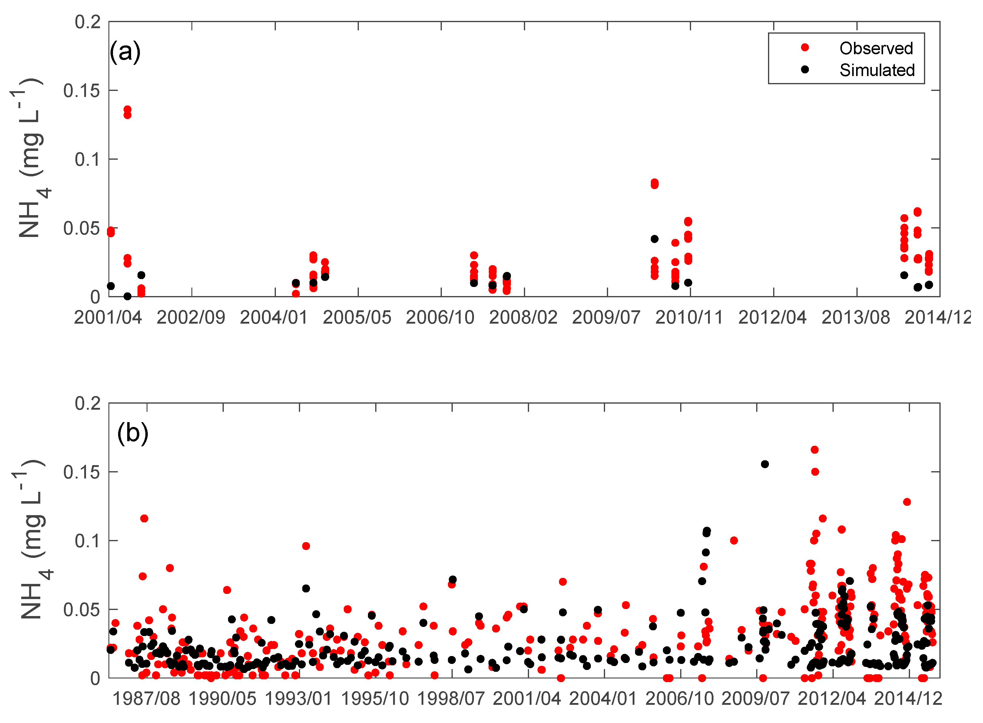
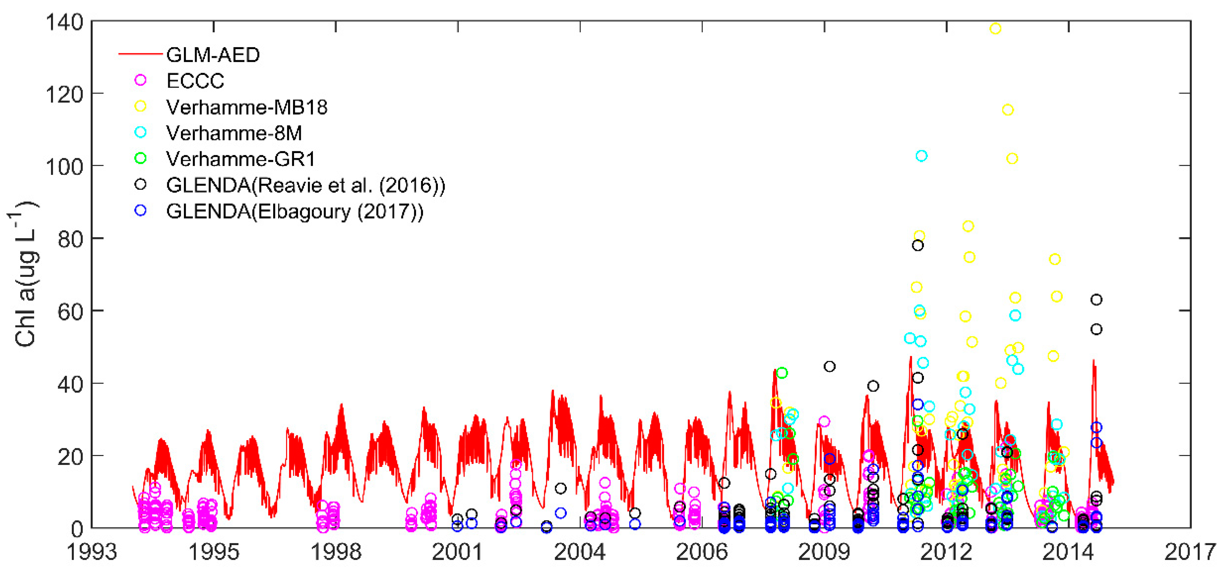
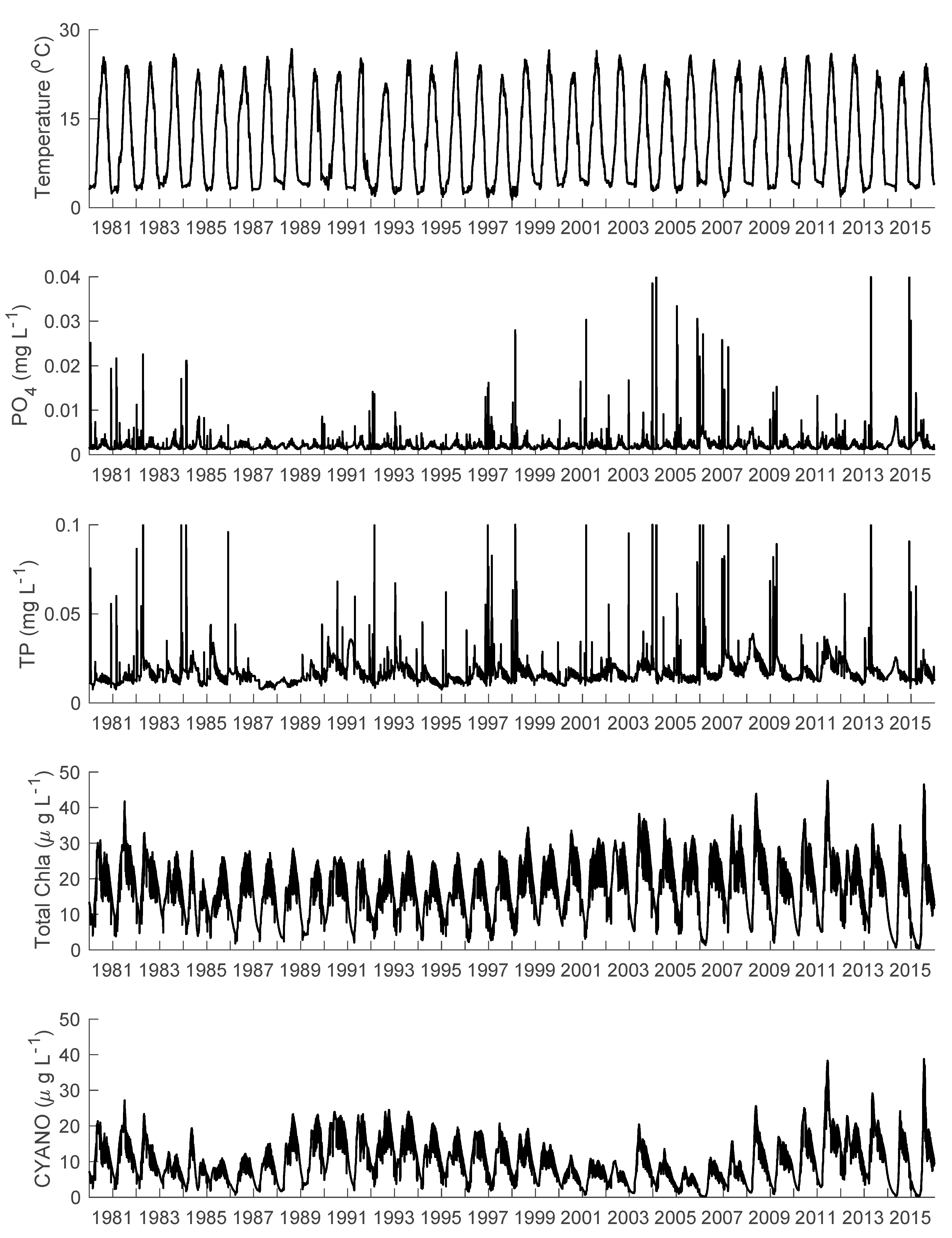
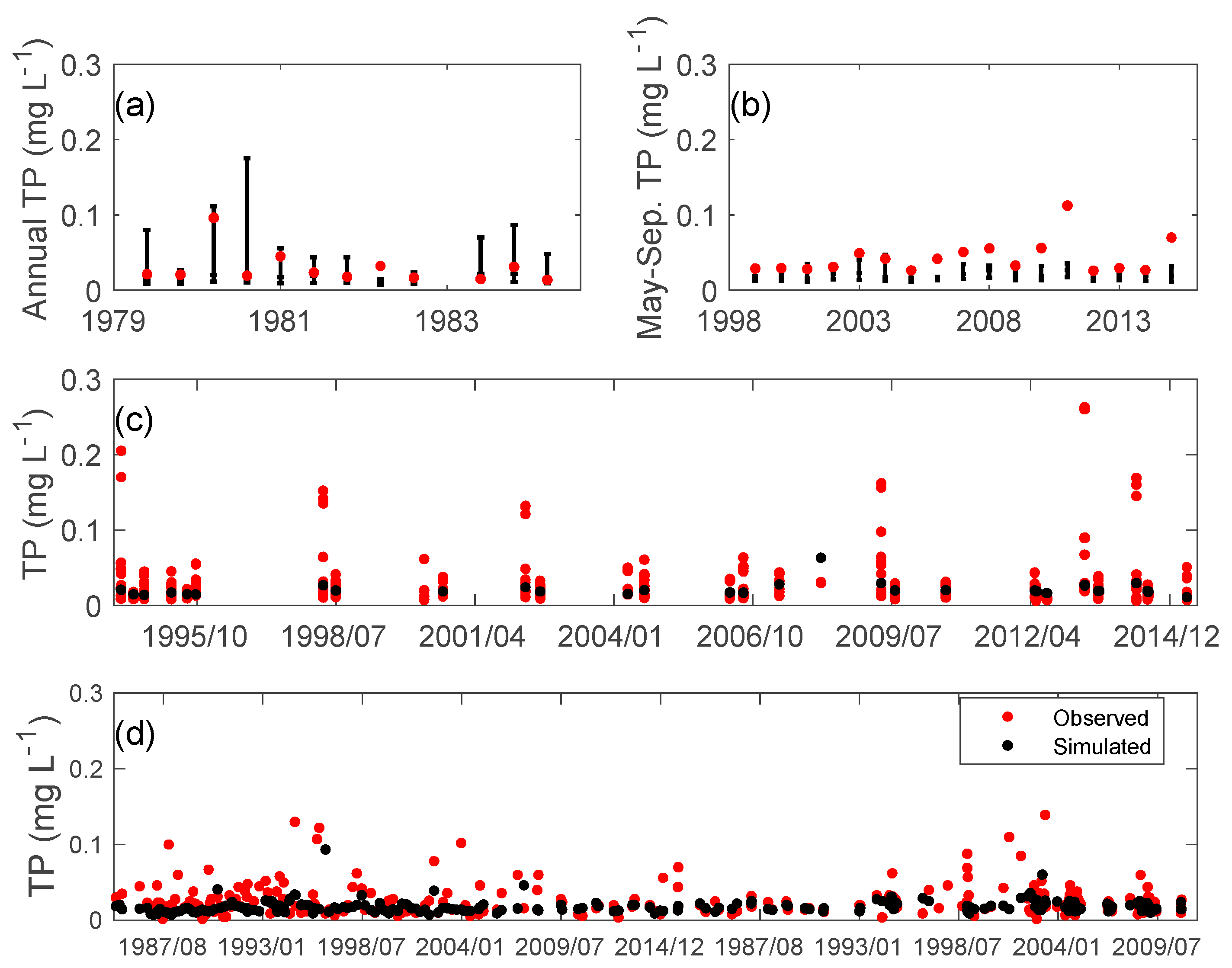
3.2. Nutrients
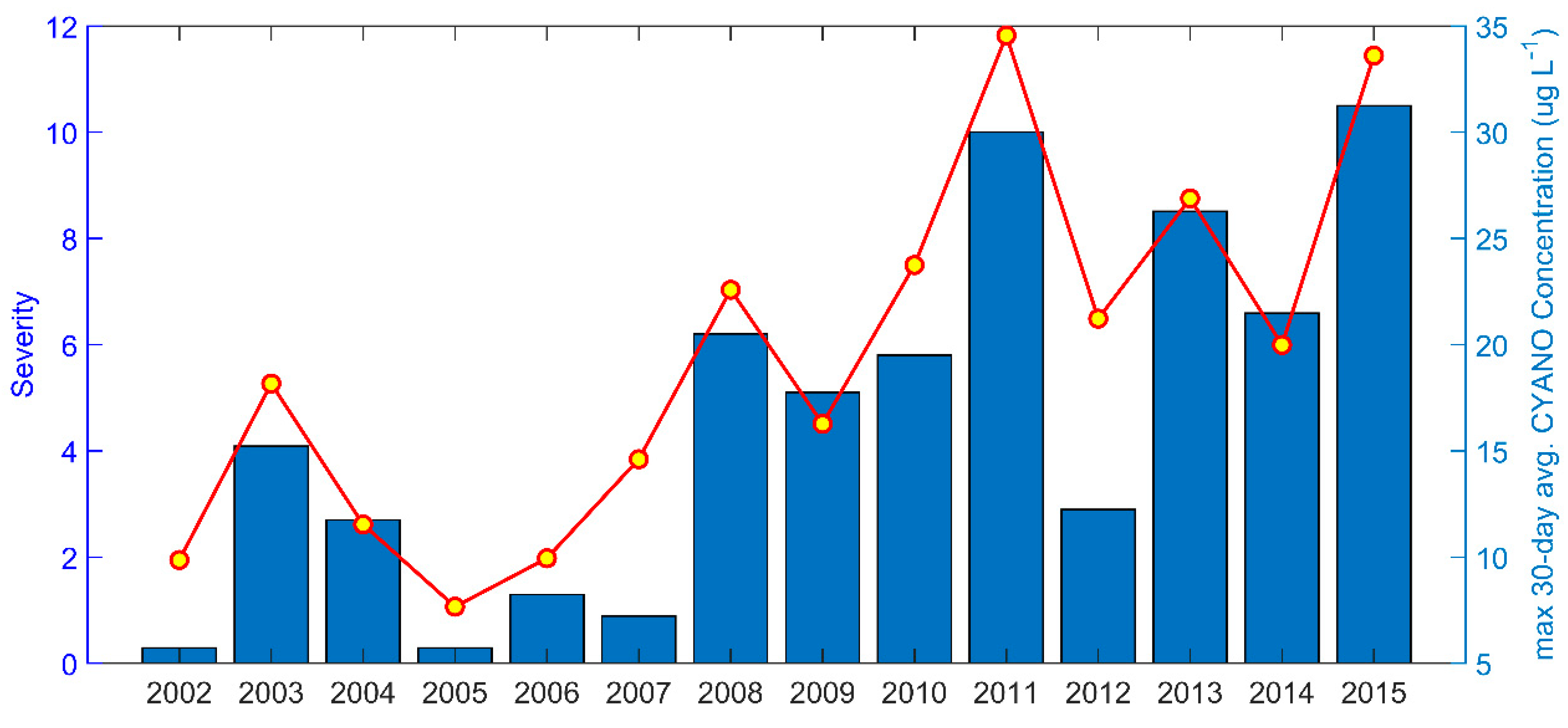
3.3. Phytoplankton
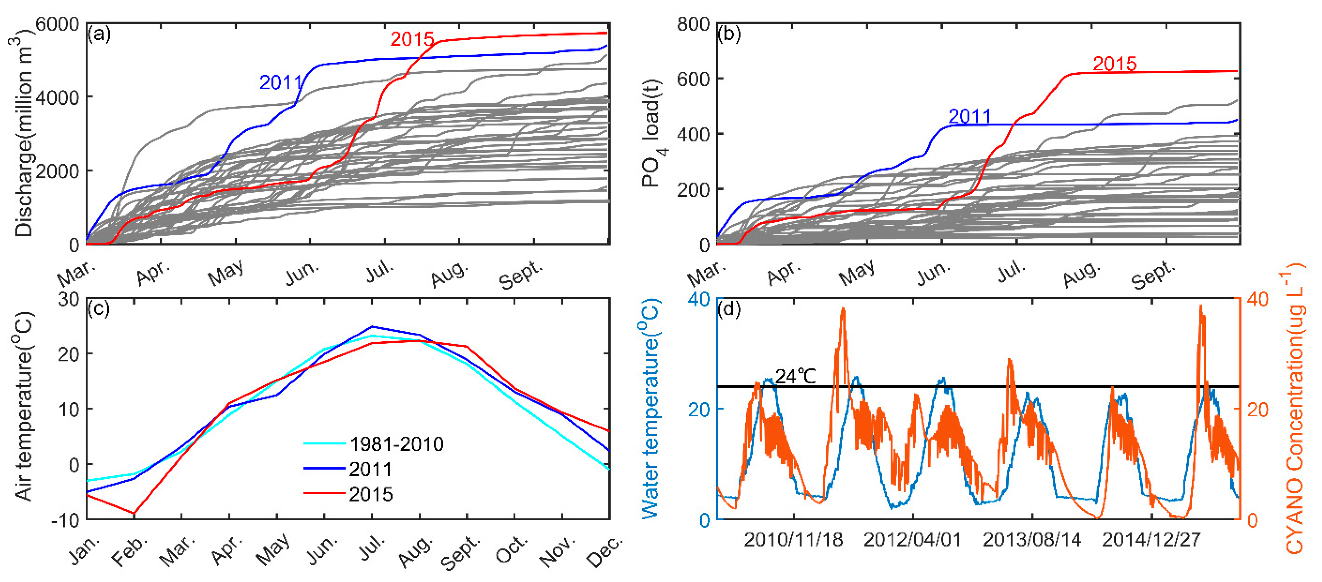
4. Discussion
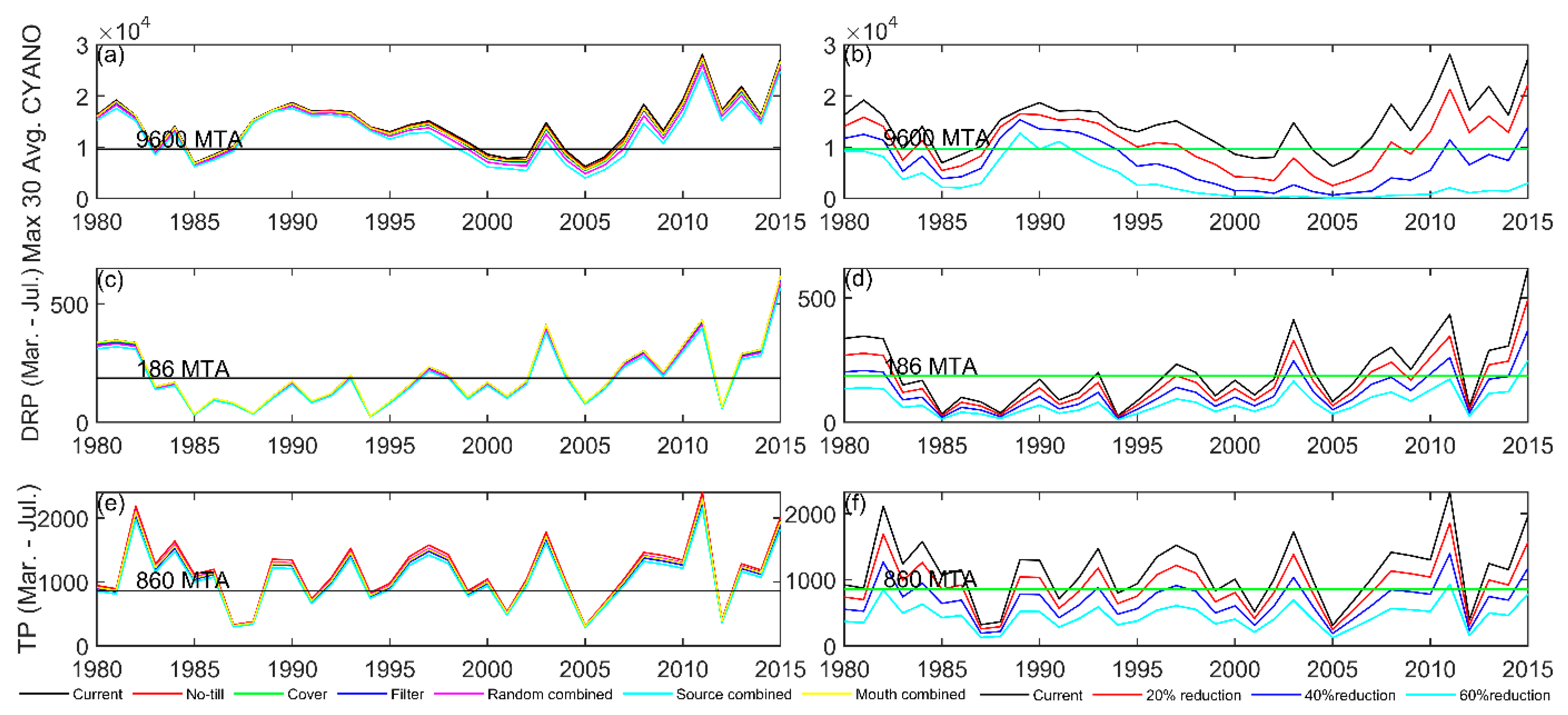
Nutrient-Reduction Scenarios
5. Conclusions
Supplementary Materials
Author Contributions
Funding
Institutional Review Board Statement
Informed Consent Statement
Data Availability Statement
Acknowledgments
Conflicts of Interest
References
- Scavia, D.; Allan, J.D.; Arend, K.K.; Bartell, S.; Beletsky, D.; Bosch, N.S.; Brandt, S.B.; Briland, R.D.; Daloğlu, I.; DePinto, J.V. Assessing and addressing the re-eutrophication of Lake Erie: Central basin hypoxia. J. Great Lakes Res. 2014, 40, 226–246. [Google Scholar] [CrossRef]
- Sweeney, R.A. “Dead” Sea of North America?—Lake Erie in the 1960s and’70s. J. Great Lakes Res. 1993, 19, 198–199. [Google Scholar] [CrossRef]
- De Pinto, J.V.; Young, T.C.; McIlroy, L.M. Great Lakes water quality improvement. Environ. Sci. Technol. 1986, 20, 752–759. [Google Scholar] [CrossRef] [PubMed]
- Dolan, D.M. Point source loadings of phosphorus to Lake Erie: 1986–1990. J. Great Lakes Res. 1993, 19, 212–223. [Google Scholar] [CrossRef]
- Makarewicz, J.C.; Bertram, P. Evidence for the restoration of the Lake Erie ecosystem. Bioscience 1991, 41, 216–223. [Google Scholar] [CrossRef] [Green Version]
- Makarewicz, J.C. Phytoplankton biomass and species composition in Lake Erie, 1970 to 1987. J. Great Lakes Res. 1993, 19, 258–274. [Google Scholar] [CrossRef]
- Millie, D.F.; Fahnenstiel, G.L.; Bressie, J.D.; Pigg, R.J.; Rediske, R.R.; Klarer, D.M.; Tester, P.A.; Litaker, R.W. Late-summer phytoplankton in western Lake Erie (Laurentian Great Lakes): Bloom distributions, toxicity, and environmental influences. Aquat. Ecol. 2009, 43, 915–934. [Google Scholar] [CrossRef] [Green Version]
- Rinta-Kanto, J.; Ouellette, A.; Boyer, G.; Twiss, M.; Bridgeman, T.; Wilhelm, S. Quantification of toxic Microcystis spp. during the 2003 and 2004 blooms in western Lake Erie using quantitative real-time PCR. Environ. Sci. Technol. 2005, 39, 4198–4205. [Google Scholar] [CrossRef]
- Kane, D.D.; Conroy, J.D.; Richards, R.P.; Baker, D.B.; Culver, D.A. Re-eutrophication of Lake Erie: Correlations between tributary nutrient loads and phytoplankton biomass. J. Great Lakes Res. 2014, 40, 496–501. [Google Scholar] [CrossRef]
- Zhang, H.; Boegman, L.; Scavia, D.; Culver, D.A. Spatial distributions of external and internal phosphorus loads in Lake Erie and their impacts on phytoplankton and water quality. J. Great Lakes Res. 2016, 42, 1212–1227. [Google Scholar] [CrossRef]
- Michalak, A.M.; Anderson, E.J.; Beletsky, D.; Boland, S.; Bosch, N.S.; Bridgeman, T.B.; Chaffin, J.D.; Cho, K.; Confesor, R.; Daloğlu, I. Record-setting algal bloom in Lake Erie caused by agricultural and meteorological trends consistent with expected future conditions. Proc. Natl. Acad. Sci. USA 2013, 110, 6448–6452. [Google Scholar] [CrossRef] [PubMed] [Green Version]
- USEPA. Recommended Phosphorus Loading Targets for Lake Erie. Annex 4 Objectives and Targets Task Team Final Report to the Nutrients Annex Subcommittee. 11 May 2015. 2015. Available online: https://www.epa.gov/sites/production/files/2015-06/documents/report-recommended-phosphorus-loading-targets-lake-erie-201505.pdf (accessed on 2 July 2021).
- Makarewicz, J.C. Nonpoint source reduction to the nearshore zone via watershed management practices: Nutrient fluxes, fate, transport and biotic responses—Background and objectives. J. Great Lakes Res. 2009, 35, 3–9. [Google Scholar] [CrossRef]
- Bosch, N.S.; Allan, J.D.; Selegean, J.P.; Scavia, D. Scenario-testing of agricultural best management practices in Lake Erie watersheds. J. Great Lakes Res. 2013, 39, 429–436. [Google Scholar] [CrossRef]
- Obenour, D.R.; Gronewold, A.D.; Stow, C.A.; Scavia, D. Using a Bayesian hierarchical model to improve Lake Erie cyanobacteria bloom forecasts. Water Resour. Res. 2014, 50, 7847–7860. [Google Scholar] [CrossRef] [Green Version]
- Bocaniov, S.A.; Smith, R.E.; Spillman, C.M.; Hipsey, M.R.; Leon, L.F. The nearshore shunt and the decline of the phytoplankton spring bloom in the Laurentian Great Lakes: Insights from a three-dimensional lake model. Hydrobiologia. 2014, 731, 151–172. [Google Scholar] [CrossRef]
- Verhamme, E.M.; Redder, T.M.; Schlea, D.A.; Grush, J.; Bratton, J.F.; DePinto, J.V. Development of the Western Lake Erie Ecosystem Model (WLEEM): Application to connect phosphorus loads to cyanobacteria biomass. J. Great Lakes Res. 2016, 42, 1193–1205. [Google Scholar] [CrossRef] [Green Version]
- Chapra, S.C.; Dolan, D.M. Great Lakes total phosphorus revisited: 2. Mass balance modeling. J. Great Lakes Res. 2012, 38, 741–754. [Google Scholar] [CrossRef]
- Leon, L.F.; Smith, R.E.; Hipsey, M.R.; Bocaniov, S.A.; Higgins, S.N.; Hecky, R.E.; Antenucci, J.P.; Imberger, J.A.; Guildford, S.J. Application of a 3D hydrodynamic–biological model for seasonal and spatial dynamics of water quality and phytoplankton in Lake Erie. J. Great Lakes Res. 2011, 37, 41–53. [Google Scholar] [CrossRef]
- Arhonditsis, G.B.; Neumann, A.; Shimoda, Y.; Kim, D.-K.; Dong, F.; Onandia, G.; Yang, C.; Javed, A.; Brady, M.; Visha, A. Castles built on sand or predictive limnology in action? Part A: Evaluation of an integrated modelling framework to guide adaptive management implementation in Lake Erie. Ecol. Inform. 2019, 53, 100968. [Google Scholar] [CrossRef]
- Elbagoury, D. Simulations of Nottawasaga River Plume. MASc Thesis, Department of Civil Engineering, Queen’s University, Kingston, ON, Canada, 2017. [Google Scholar]
- Nakhaei, N. Computational and Empirical Water Quality Modeling in Lakes and Ponds. Ph.D. Thesis, Department of Civil Engineering, Queen’s University, Kingston, ON, Canada, 2017. [Google Scholar]
- Hipsey, M.R.; Bruce, L.C.; Boon, C.; Busch, B.; Carey, C.C.; Hamilton, D.P.; Hanson, P.C.; Read, J.S.; De Sousa, E.; Weber, M. A General Lake Model (GLM 3.0) for linking with high-frequency sensor data from the Global Lake Ecological Observatory Network (GLEON). Geosci. Model Dev. 2019, 473–523. [Google Scholar] [CrossRef] [Green Version]
- Gaudard, A.; Råman Vinnå, L.; Bärenbold, F.; Schmid, M.; Bouffard, D. Toward an open access to high-frequency lake modeling and statistics data for scientists and practitioners–the case of Swiss lakes using Simstrat v2. 1. Geosci. Model Dev. 2019, 12. [Google Scholar] [CrossRef] [Green Version]
- Tyson, J.; Davies, D.; Mackey, S. Influence of riverine inflows on western Lake Erie: Implications for fisheries management. In Proceedings of the 12th Biennial Coastal Zone Conference, Cleveland, OH, USA; 2001. [Google Scholar]
- Matisoff, G.; Kaltenberg, E.M.; Steely, R.L.; Hummel, S.K.; Seo, J.; Gibbons, K.J.; Bridgeman, T.B.; Seo, Y.; Behbahani, M.; James, W.F. Internal loading of phosphorus in western Lake Erie. J. Great Lakes Res. 2016, 42, 775–788. [Google Scholar] [CrossRef]
- Ackerman, J.D.; Loewen, M.R.; Hamblin, P.F. Benthic-pelagic coupling over a zebra mussel reef in western Lake Erie. Limnol. Oceanogr. 2001, 46, 892–904. [Google Scholar] [CrossRef]
- Ludsin, S.A.; Kershner, M.W.; Blocksom, K.A.; Knight, R.L.; Stein, R.A. Life after death in Lake Erie: Nutrient controls drive fish species richness, rehabilitation. Ecol. Appl. 2001, 11, 731–746. [Google Scholar] [CrossRef]
- Thomas, M.; Biesinger, Z.; Deller, J.; Hosack, M.; Kocovsky, P.; MacDougall, T.; Markham, J.; Perez-Fuentetaja, A.; Weimer, E.; Witzel, L. Report of the Lake Erie Forage Task Group. Lake Erie Comm. March 2014. [Google Scholar]
- Reavie, E.D.; Cai, M.; Twiss, M.R.; Carrick, H.J.; Davis, T.W.; Johengen, T.H.; Gossiaux, D.; Smith, D.E.; Palladino, D.; Burtner, A. Winter–spring diatom production in Lake Erie is an important driver of summer hypoxia. J. Great Lakes Res. 2016, 42, 608–618. [Google Scholar] [CrossRef]
- Hamilton, D.P.; Schladow, S.G. Prediction of water quality in lakes and reservoirs. Part I—Model description. Ecol. Modell. 1997, 96, 91–110. [Google Scholar] [CrossRef]
- Trolle, D.; Skovgaard, H.; Jeppesen, E. The Water Framework Directive: Setting the phosphorus loading target for a deep lake in Denmark using the 1D lake ecosystem model DYRESM–CAEDYM. Ecol. Modell. 2008, 219, 138–152. [Google Scholar] [CrossRef]
- Snortheim, C.A.; Hanson, P.C.; McMahon, K.D.; Read, J.S.; Carey, C.C.; Dugan, H.A. Meteorological drivers of hypolimnetic anoxia in a eutrophic, north temperate lake. Ecol. Modell. 2017, 343, 39–53. [Google Scholar] [CrossRef] [Green Version]
- Weber, M.; Rinke, K.; Hipsey, M.; Boehrer, B. Optimizing withdrawal from drinking water reservoirs to reduce downstream temperature pollution and reservoir hypoxia. J. Environ. Manage. 2017, 197, 96–105. [Google Scholar] [CrossRef] [PubMed]
- Hipsey, M.; Bruce, L.; Hamilton, D. Aquatic Ecodynamics (AED) Model Library Science Manual; Perth, Australia; p. 2013. Available online: https://aed.see.uwa.edu.au/research/models/AED/Download/AED_ScienceManual_v4_draft.pdf (accessed on 2 July 2021).
- Boegman, L.; Loewen, M.R.; Culver, D.A.; Hamblin, P.F.; Charlton, M.N. Spatial-Dynamic Modeling of Algal Biomass in Lake Erie: Relative Impacts of Dreissenid Mussels and Nutrient Loads. J. Environ. Eng. ASCE 2008, 134, 456–468. [Google Scholar] [CrossRef] [Green Version]
- Gibson, J.; Prowse, T.; Peters, D. Hydroclimatic controls on water balance and water level variability in Great Slave Lake. Hydrol. Process. 2006, 20, 4155–4172. [Google Scholar] [CrossRef]
- Kebede, S.; Travi, Y.; Alemayehu, T.; Marc, V. Water balance of Lake Tana and its sensitivity to fluctuations in rainfall, Blue Nile basin, Ethiopia. J. Hydrol. 2006, 316, 233–247. [Google Scholar] [CrossRef]
- Luo, L.; Hamilton, D.; Lan, J.; McBride, C.; Trolle, D. Autocalibration of a one-dimensional hydrodynamic-ecological model (DYRESM 4.0-CAEDYM 3.1) using a Monte Carlo approach: Simulations of hypoxic events in a polymictic lake. Geosci. Model Dev. 2018, 11, 903–913. [Google Scholar] [CrossRef] [Green Version]
- Zhang, W.; Rao, Y.R. Application of a eutrophication model for assessing water quality in Lake Winnipeg. J. Great Lakes Res. 2012, 38, 158–173. [Google Scholar] [CrossRef]
- Bosch, N.S.; Evans, M.A.; Scavia, D.; Allan, J.D. Interacting effects of climate change and agricultural BMPs on nutrient runoff entering Lake Erie. J. Great Lakes Res. 2014, 40, 581–589. [Google Scholar] [CrossRef]
- Scavia, D.; Kalcic, M.; Muenich, R.L.; Aloysius, N.; Arnold, J.; Boles, C.; Confessor, R.; De Pinto, J.; Gildow, M.; Martin, J. Informing Lake Erie Agriculture Nutrient Management via Scenario Evaluation; University of Michigan: Ann Arbor, MI, USA, 2016. [Google Scholar]
- Chapra, S.C. Total Phosphorus Model for the Great Lakes. J. Environ. Eng. Div. ASCE 1977, 103, 147–161. [Google Scholar] [CrossRef]
- Wetzel, R.G. Limnology: Lake and River Ecosystems, 3rd ed.; Academic Press: Cambridge, MA, USA, 2001. [Google Scholar]
- Boegman, L.; Sleep, S. Feasibility of bubble plume destratification of central Lake Erie. J. Hydraul. Eng. 2012, 138, 985–989. [Google Scholar] [CrossRef]
- Liu, W.; Bocaniov, S.A.; Lamb, K.G.; Smith, R.E. Three dimensional modeling of the effects of changes in meteorological forcing on the thermal structure of Lake Erie. J. Great Lakes Res. 2014, 40, 827–840. [Google Scholar] [CrossRef]
- Bruce, L.C.; Frassl, M.A.; Arhonditsis, G.B.; Gal, G.; Hamilton, D.P.; Hanson, P.C.; Hetherington, A.L.; Melack, J.M.; Read, J.S.; Rinke, K.; et al. A multi-lake comparative analysis of the General Lake Model (GLM): Stress-testing across a global observatory network. Environ. Model. Softw. 2018, 102, 274–291. [Google Scholar] [CrossRef] [Green Version]
- Collier, K.M. Partitioning of Phytoplankton and Bacteria between Water and Ice during Winter in North Temperate Lakes. MS Thesis, Bowling Green State University, Bowling Green, OH, USA, 2016. [Google Scholar]
- Bocaniov, S.A.; Scavia, D. Temporal and spatial dynamics of large lake hypoxia: Integrating statistical and three-dimensional dynamic models to enhance lake management criteria. Water Resour. Res. 2016, 52, 4247–4263. [Google Scholar] [CrossRef] [Green Version]
- Ohio Lake Erie Phosphorus Task Force II. Final Report. The Lake Erie Commission, Ann Arbor, Ohio. 2013. Available online: https://www.epa.ohio.gov/portals/35/lakeerie/ptaskforce2/Task_Force_Report_October_2013.pdf (accessed on 2 July 2021).
- Chaffin, J.D.; Bridgeman, T.B.; Bade, D.L. Nitrogen constrains the growth of late summer cyanobacterial blooms in Lake Erie. Adv. Microbiol. 2013, 2013. [Google Scholar] [CrossRef] [Green Version]
- Wynne, T.T.; Stumpf, R.P. Spatial and temporal patterns in the seasonal distribution of toxic cyanobacteria in western Lake Erie from 2002–2014. Toxins 2015, 7, 1649–1663. [Google Scholar] [CrossRef] [PubMed] [Green Version]
- Wynne, T.; Stumpf, R.; Tomlinson, M.; Warner, R.; Tester, P.; Dyble, J.; Fahnenstiel, G. Relating spectral shape to cyanobacterial blooms in the Laurentian Great Lakes. Int. J. Remote Sens. 2008, 29, 3665–3672. [Google Scholar] [CrossRef]
- Wynne, T.T.; Stumpf, R.P.; Tomlinson, M.C.; Dyble, J. Characterizing a cyanobacterial bloom in western Lake Erie using satellite imagery and meteorological data. Limnol. Oceanogr. 2010, 55, 2025–2036. [Google Scholar] [CrossRef] [Green Version]
- Stumpf, R.P.; Wynne, T.T.; Baker, D.B.; Fahnenstiel, G.L. Interannual variability of cyanobacterial blooms in Lake Erie. PloS ONE 2012, 7, e42444. [Google Scholar] [CrossRef]
- Scavia, D.; DePinto, J.; Auer, M.; Bertani, I.; Bocaniov, S.; Chapra, S.; Leon, L.; McCrimmon, C.; Obenour, D.; Peterson, G. Great Lakes Water Quality Agreement Nutrient Annex Objectives and Targets Task Team Ensemble Multi-Modeling Report; Great Lakes National Program Office, USEPA: Chicago, IL, USA, 2016. [Google Scholar]
- Baker, D.B.; Johnson, L.T.; Confesor Jr, R.B.; Crumrine, J.P.; Guo, T.; Manning, N.F. Needed: Early-term adjustments for Lake Erie phosphorus target loads to address western basin cyanobacterial blooms. J. Great Lakes Res. 2019, 45, 203–211. [Google Scholar] [CrossRef]
- Richards, R.; Baker, D.; Crumrine, J.; Stearns, A. Unusually large loads in 2007 from the Maumee and Sandusky Rivers, tributaries to Lake Erie. J. Soil Water Conserv. 2010, 65, 450–462. [Google Scholar] [CrossRef] [Green Version]
- Baker, D.; Confesor, R.; Ewing, D.; Johnson, L.; Kramer, J.; Merryfield, B. Phosphorus loading to Lake Erie from the Maumee, Sandusky and Cuyahoga rivers: The importance of bioavailability. J. Great Lakes Res. 2014, 40, 502–517. [Google Scholar] [CrossRef]
- Bridgeman, T.B.; Chaffin, J.D.; Filbrun, J.E. A novel method for tracking western Lake Erie Microcystis blooms, 2002–2011. J. Great Lakes Res. 2013, 39, 83–89. [Google Scholar] [CrossRef]
- Moore, S.K.; Trainer, V.L.; Mantua, N.J.; Parker, M.S.; Laws, E.A.; Backer, L.C.; Fleming, L.E. Impacts of climate variability and future climate change on harmful algal blooms and human health. Environ. Health 2008, 7, S4. [Google Scholar] [CrossRef] [PubMed] [Green Version]
- Paerl, H.W.; Huisman, J. Blooms like it hot. Science 2008, 320, 57–58. [Google Scholar] [CrossRef] [Green Version]
- Schindler, D.W.; Hecky, R.; Findlay, D.; Stainton, M.; Parker, B.; Paterson, M.; Beaty, K.; Lyng, M.; Kasian, S. Eutrophication of lakes cannot be controlled by reducing nitrogen input: Results of a 37-year whole-ecosystem experiment. Proc. Natl. Acad. Sci. USA 2008, 105, 11254–11258. [Google Scholar] [CrossRef] [PubMed] [Green Version]
- Daloglu, I.; Cho, K.H.; Scavia, D. Evaluating causes of trends in long-term dissolved reactive phosphorus loads to Lake Erie. Environ. Sci. Technol. 2012, 46, 10660–10666. [Google Scholar] [CrossRef] [PubMed]
- Hipsey, M.; Bruce, L.; Hamilton, D. Aquatic Ecodynamics (AED) Model Library Science Manual; The University of Western Australia Technical Manual: Perth, Australia, 2013; Volume 34. [Google Scholar]
- Scavia, D.; Kalcic, M.; Muenich, R.; Aloysius, N.; Arnold, J.; Boles, C.; Confessor, R.; De Pinto, J.; Gildow, M.; Martin, J. Informing Lake Erie Agriculture Nutrient Management via Scenario Evaluation; University of Michigan Water Center: Ann Arbor, MI, USA, 2016. [Google Scholar]
- Hartig, J.H.; Wallen, D.G. Seasonal variation of nutrient limitation in western Lake Erie. J. Great Lakes Res. 1984, 10, 449–460. [Google Scholar] [CrossRef]
- Chaffin, J.D.; Bridgeman, T.B.; Bade, D.L.; Mobilian, C.N. Summer phytoplankton nutrient limitation in Maumee Bay of Lake Erie during high-flow and low-flow years. J. Great Lakes Res. 2014, 40, 524–531. [Google Scholar] [CrossRef]
- Özkundakci, D.; Hamilton, D.P.; Trolle, D. Modelling the response of a highly eutrophic lake to reductions in external and internal nutrient loading. N. Zeal. J. Mar. Fresh. 2011, 45, 165–185. [Google Scholar] [CrossRef]


| HFCB | harmful cyanobacteria |
| AED | Aquatic Ecosystem Dynamics |
| GLM | General Lake Model |
| P | phosphorus |
| N | nitrogen |
| PEST | Model-Independent Parameter Estimation |
| GLWQA | Great Lakes Water Quality Agreement |
| TP | total phosphorus |
| DRP | dissolved reactive phosphorus |
| USEPA | United States Environmental Protection Agency |
| BMP | agricultural best management practice |
| Chl-a | total chlorophyll a |
| MTA | metric tons per annum |
| ELCOM | Estuary and Lake Computer Model |
| CAEDYM | Computational Aquatic Ecosystem Model |
| WLEEM | Western Lake Erie Ecosystem Model |
| EcoLE | Ecological Model of Lake Erie |
| GLERL | Great Lakes Environmental Research Laboratory |
| NOAA | National Oceanic and Atmospheric Administration |
| ECCC | Environment and Climate Change Canada |
| EMRB | Environmental Monitoring and Reporting Branch |
| OCWA | Ontario Clean Water Agency |
| GLENDA | Great Lakes Environmental Database |
| NDBC | National Data Buoy Centre |
| GREEN | green algae |
| CYANO | cyanobacteria |
| DIAT | diatoms |
| CRYPT | cryptophytes |
| DO | dissolved oxygen |
| PO4 | dissolved reactive phosphorus |
| NO3 | nitrate |
| NH4 | ammonium |
| RSi | reactive silica |
| DON | dissolved organic nitrogen |
| DOP | dissolved organic phosphorus |
| DOC | dissolved organic carbon |
| PON | particulate organic nitrogen |
| POP | particulate organic phosphorus |
| POC | particulate organic carbon |
| RS | relative sensitivity |
| ARS | absolute relative sensitivity |
| RMSE | root-mean-square error |
| DYRESM | Dynamic Reservoir Simulation Model |
| SWAT | Soil and Water Assessment Tool |
| CI | cyanobacteria index |
| WASP | Water Quality Analysis Simulation Program |
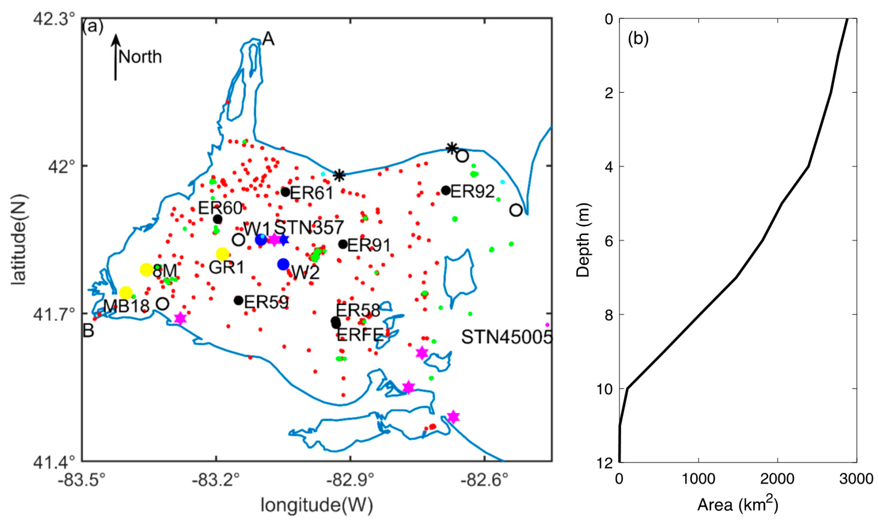
| Character | Location | Source | Identifier in Figure 1 | Sample Date |
|---|---|---|---|---|
| Water temperature | Western basin surface and Sta. 45005 | ECCC and NOAA & NDBC | Red and magenta dots | 1979–2015 and 2005–2015 |
| Sta. W1, W2 and Sta. 357 | Ackerman et al. (2001) | Blue circles and star | 1994 and 2008 | |
| Nutrients (phosphorus and nitrogen) | Western basin | Ludsin et al. (2001) | Orange diamond | 1980–1992 |
| Western basin | Thomas et al. (2014) | Black circles | 1999–2015 (May–Sep.) | |
| 1–11 m | ECCC | Green dots | 1994–2015 | |
| 0–18.8 m | OCWA | Cyan dots | 2001–2014 | |
| 1 m above bottom | EMRB | Black asterisks | 1986–2015 | |
| ER58 (integrated sample) | GLENDA | Black dots | 1986–2015 | |
| ER59 (integrated sample) | ||||
| ER60 (integrated sample) | ||||
| ER61 (integrated sample) | ||||
| ER91 (integrated sample) | ||||
| ER92 (integrated sample) | ||||
| Chl-a | 1–11m depth | ECCC | Green dots | 1994–2015 |
| MB18 (integrated sample) | Verhamme et al. (2016) | Yellow dots | 2008–2014 | |
| 8M (integrated sample) | ||||
| GR1 (integrated sample) | ||||
| ER58 (integrated sample) | GLENDA | Black dots | 2001–2015 | |
| ER59 (integrated sample) | ||||
| ER60 (integrated sample) | ||||
| ER61 (integrated sample) | ||||
| ER91 (integrated sample) | ||||
| ER92 (integrated sample) | ||||
| Phytoplankton groups | ER58 (integrated sample) | GLENDA | Black dots | 2001–2015 |
| ER59 (integrated sample) | ||||
| ER60 (integrated sample) | ||||
| ER61 (integrated sample) | ||||
| ER91 (integrated sample) | ||||
| ER92 (integrated sample) |
| DO (mmol O2/m3) | SiO2 (mmol Si/m3) | NH4 (mmol N/m3) | NO3 (mmol N/m3) | PO4 (mmol P/m3) | PON (mmol N/m3) | DON (mmol N/m3) | POP (mmol P/m3) |
|---|---|---|---|---|---|---|---|
| 376.76 | 114.29 | 9.66 | 47.42 | 2.97 | 30.18 | 80.88 | 3.48 |
| DOP (mmol P/m3) | POC (mmol C/m3) | DOC (mmol C/m3) | GREEN (mmol C/m3) | DIAT (mmol C/m3) | CYANO (mmol C/m3) | CRYPT (mmol C/m3) | |
| 2.32 | 41.67 | 250 | 1.59 | 1.81 | 0 | 0.03 |
| Model Parameter | ARS of Modelled State Variable | |||||||
|---|---|---|---|---|---|---|---|---|
| Water Temperature | PO4 | TP | Chl-a | GREEN | CYANO | DIAT | CRYPT | |
| 0.02 | 0.37 | 0.09 | 0.86 | 4.89 | 3.19 | 0.58 | 4.6 | |
| 0.06 | 0.28 | 0.07 | 0.35 | 0.66 | 0.93 | 0.66 | 0.22 | |
| 0.66 | 0.32 | 0.24 | 0.78 | 2.62 | 5.50 | 2.58 | 12.88 | |
| 0.01 | -- | -- | -- | -- | -- | -- | -- | |
| 0.01 | -- | -- | -- | -- | -- | -- | -- | |
| 0.01 | -- | -- | -- | -- | -- | -- | -- | |
| -- | 0.65 | 0.07 | -- | -- | -- | -- | -- | |
| -- | 0.29 | 0.15 | 0.31 | 1.25 | 2.20 | 0.02 | 1.06 | |
| -- | 0.25 | 0.13 | 0.26 | 1.06 | 1.87 | 0.03 | 0.91 | |
| -- | 0.24 | 0.06 | 0.75 | 20.70 | 7.69 | 2.49 | 8.29 | |
| -- | 0.03 | 0.03 | 0.30 | 9.80 | 4.98 | 0.06 | 8.44 | |
| -- | 0.08 | 0.05 | 0.60 | 14.44 | 7.94 | 0.29 | 7.31 | |
| -- | 0.05 | 0.04 | 0.45 | 11.89 | 6.58 | 0.21 | 6.40 | |
| -- | 0.01 | 0.01 | 0.16 | 9.67 | 2.58 | 0.04 | 2.90 | |
| -- | 0.02 | 0.03 | 0.30 | 9.50 | 4.80 | 0.03 | 8.19 | |
| -- | 0.23 | 0.04 | 0.72 | 9.39 | 12.94 | 2.48 | 8.60 | |
| -- | 0.03 | 0.04 | 0.52 | 8.31 | 9.53 | 0.05 | 15.98 | |
| -- | 0.004 | 0.03 | 0.35 | 8.18 | 8.49 | 0.02 | 6.89 | |
| -- | 0.004 | 0.03 | 0.30 | 6.53 | 8.89 | 0.03 | 5.39 | |
| -- | 0.001 | 0.01 | 0.07 | 1.36 | 8.26 | 0.02 | 1.36 | |
| -- | 0.002 | 0.04 | 0.45 | 7.87 | 8.96 | 0.13 | 15.10 | |
| -- | 0.13 | 0.02 | 0.65 | 0.27 | 0.88 | 3.50 | 0.24 | |
| -- | 0.001 | 0.06 | 0.05 | 1.76 | 2.69 | 9.93 | 0.96 | |
| -- | 0.01 | 0.002 | 0.05 | 0.15 | 0.01 | 3.32 | 0.12 | |
| -- | 0.02 | 0.003 | 0.12 | 0.47 | 0.11 | 3.82 | 0.40 | |
| -- | 0.10 | 0.01 | 0.38 | 1.93 | 0.57 | 2.94 | 1.84 | |
| -- | 0.11 | 0.03 | 0.60 | 0.77 | 0.55 | 3.48 | 0.56 | |
| ---- | 0.24 | 0.07 | 0.73 | 9.24 | 7.63 | 2.48 | 83.71 | |
| -- | 0.01 | 0.01 | 0.06 | 1.44 | 1.09 | 0.03 | 16.65 | |
| -- | 0.07 | 0.05 | 0.58 | 8.67 | 7.72 | 0.28 | 64.43 | |
| -- | 0.05 | 0.04 | 0.47 | 8.21 | 6.72 | 0.21 | 57.72 | |
| -- | 0.008 | 0.01 | 0.12 | 2.92 | 1.91 | 0.03 | 17.90 | |
| -- | 0.004 | 0.01 | 0.07 | 1.38 | 1.01 | 0.001 | 16.98 | |
| Scenario Name | Scenario Description | Change in TP Load (%) | Change PO4 Load (%) |
|---|---|---|---|
| No-till | No-till corn and soybean implemented in random 25% of row-crop agricultural land | +2.46 | −1.54 |
| Cover | Rye cover crop planted between soybean and corn crop in random 25% of row-crop agricultural land | −2.37 | −1.66 |
| Filter | Filter strip (10 m with 25% trapping efficiency) in random 20% of row-crop agricultural land | −2.97 | −3.08 |
| Random combined | Combination of three BMPs on same 25% of Maumee row-crop agricultural land; randomly distributed among sub-watersheds | −0.88 | −4.41 |
| Source combined | Combination of three BMPs on same 25% of Maumee row-crop agricultural land; distributed in high source sub-watersheds | −6.92 | −8.04 |
| Mouth combined | Combination of three BMPs on same 25% of Maumee row-crop agricultural land; distributed in sub-watersheds near river mouth | −0.86 | −0.18 |
| BMP Scenarios | TP (mmol m−3) | PO4 (mmol m−3) | TN (mmol m−3) | NO3 (mmol m−3) | Chl-a (μg L−1) | CYANO (μg L−1) |
|---|---|---|---|---|---|---|
| Baseline | 0.56 | 0.07 | 63.54 | 32.84 | 17.58 | 10.17 |
| No-till | 0.57 | 0.07 | 63.70 | 32.98 | 17.56 | 9.96 |
| Cover | 0.55 | 0.07 | 62.84 | 32.43 | 17.55 | 9.76 |
| Filter | 0.55 | 0.07 | 63.15 | 32.65 | 17.54 | 9.80 |
| Random combined | 0.56 | 0.07 | 62.74 | 32.38 | 17.51 | 9.42 |
| Source combined | 0.54 | 0.07 | 62.28 | 32.17 | 17.46 | 8.93 |
| Mouth combined | 0.55 | 0.07 | 62.90 | 32.54 | 17.56 | 9.87 |
Publisher’s Note: MDPI stays neutral with regard to jurisdictional claims in published maps and institutional affiliations. |
© 2021 by the authors. Licensee MDPI, Basel, Switzerland. This article is an open access article distributed under the terms and conditions of the Creative Commons Attribution (CC BY) license (https://creativecommons.org/licenses/by/4.0/).
Share and Cite
Wang, Q.; Boegman, L. Multi-Year Simulation of Western Lake Erie Hydrodynamics and Biogeochemistry to Evaluate Nutrient Management Scenarios. Sustainability 2021, 13, 7516. https://doi.org/10.3390/su13147516
Wang Q, Boegman L. Multi-Year Simulation of Western Lake Erie Hydrodynamics and Biogeochemistry to Evaluate Nutrient Management Scenarios. Sustainability. 2021; 13(14):7516. https://doi.org/10.3390/su13147516
Chicago/Turabian StyleWang, Qi, and Leon Boegman. 2021. "Multi-Year Simulation of Western Lake Erie Hydrodynamics and Biogeochemistry to Evaluate Nutrient Management Scenarios" Sustainability 13, no. 14: 7516. https://doi.org/10.3390/su13147516
APA StyleWang, Q., & Boegman, L. (2021). Multi-Year Simulation of Western Lake Erie Hydrodynamics and Biogeochemistry to Evaluate Nutrient Management Scenarios. Sustainability, 13(14), 7516. https://doi.org/10.3390/su13147516