Abstract
This article reports on the relation between the surface topography and the optical reflectance, both total and diffuse, of different samples of AISI 430 ferritic stainless steel. Gaussian filters with different cutoff wavelengths were applied to the height maps of the surface topography of the samples, to separate the different scales of surface roughness involved in optical scattering in the visible range of the spectrum. Significant anisotropy, related to the rolling process, was found in the topography. An effective roughness slope parameter was defined from the dependence of the ratio between the root mean square height and the autocorrelation length on the cutoff wavelength. This roughness slope demonstrated an exceptionally good linear relationship with CIE 1931 luminance, which was calculated from the diffuse reflection spectra. The color uniformity of the samples was analyzed based on their CIE L*a*b* coordinates under daylight and LED illumination. The results confirmed the strong influence of manufacturing process on the surface characteristics of AISI 430 ferritic stainless steel sheet products with a bright finish.
1. Introduction
Quality control of the visual appearance of surfaces is a key issue in industrial fields dealing with paints, coatings, texturing, and finishing [1,2,3,4,5,6,7]. The optical scattering distribution function is a topic of interest in engineering applications such as the manufacture of high-quality mirrors for scientific use [8], and knowledge of this topic has been supported by the development of infographics and surface rendering [9,10,11,12]. A number of theoretical approaches developed to model the bidirectional reflectance distribution function (BRDF) and the most complete bidirectional scattering-surface reflectance distribution function (BSSRDF) is presented in the review by Frisvad et al. [13], which provides a comprehensive analysis of the approaches that can be found in the literature.
In all these theoretical models, the topographical characteristics of the surface are related in some way to the angular distribution of the light reflected by a surface. All of them have limitations in the goodness of the model according to the roughness scale. Some of these models explicitly consider surface microgeometry, making them better suited to modelling the optical scattering produced by small-scale (nano/micro) roughness. These models are based on the Rayleigh–Rice approach [14,15] and are valid for smooth surfaces fulfilling the so-called Rayleigh criterion:
where Sq stands for the root mean square height of the surface topography, θi is the incidence angle of the light on the surface, and λ is the light wavelength. Other models, based on the Beckmann–Kirchhoff theory, approximate the topography using a normal distribution of microfacets and are better suited to modelling the optical scattering produced by surfaces with roughness on the micro/milli scale [11,15,16,17,18,19].
The aim of the present paper is to characterize the visual appearance of AISI 430 ferritic stainless steel sheets with a bright finish. This product has been commercialized for applications in the manufacturing of home electrical appliances, cutlery, indoor decorations, and other household goods. The production line involves several steps of rolling and bright annealing that lead to a certain variability in the visual appearance of products from different batches. This makes it necessary to establish unambiguous testing processes to characterize and determine the quality of the commercial product.
This work reports on the topographic and photometric characterization of a set of AISI 430 ferritic stainless steel samples from different production batches. It analyzes the effect of applying a Gaussian filter to the topographic maps on the determination of the values of the areal roughness parameters relevant to optical scattering. Special attention is paid to the root mean square height, Sq, and the autocorrelation length, Sal, as well as the slope, Sq/Sal. The results show that there is a strong relationship between the slope and the photometric luminance coordinate of the samples. Additionally, the article reports on color coordinates in the CIE L*a*b* color space, and discusses the color uniformity of the samples.
2. Materials and Methods
2.1. Materials and Bright Annealing
The AISI 430 ferritic stainless steel products studied in this work were produced in flat sheet form with thickness in the range of 0.40–1.50 mm, under conventional industrial conditions, using an electric arc furnace, an AOD converter, and continuous casting [20]. The reduction in slab thickness took place during hot rolling, and the material was recrystallized at the end of this stage by means of an annealing treatment. After this, the final thickness of the coil was reached via a cold rolling stage. A final annealing process was performed in a reducing atmosphere to recrystallize the structure of the steel and, therefore, remove any internal structural alterations produced during the rolling process. In addition, a bright finish was achieved during this stage due to the non-alteration of the laminated surface under the annealing furnace’s H2/N2 atmosphere. The surface of the sheet was not polished before annealing. More details about the production process can be found at www.acerinox.com (accessed on 1 June 2021).
The chemical composition of the AISI 430 ferritic stainless steel samples under study is given in Table 1. It corresponds to the symbolic designation X6Cr17 and numerical designation 1.4016, according to the EN 10088-2 standard [21].

Table 1.
Chemical composition of the AISI 430 ferritic stainless steel samples under study.
The grain size of the AISI 430 stainless steel specimens was found to be between 7.9 μm and 13.4 μm. The average grain size was 11.3 µm, which corresponds to a G index of 10, according to ASTM E 112 [22]. The mechanical properties of this material after cold rolling and final annealing, as specified in [21], were:
- Yield strength, Rp0.2 > 260 MPa;
- Tensile strength, Rm = 450–600 MPa;
- Elongation > 25%;
- Hardness < 185 HB;
- Modulus of elasticity at 20 °C = 220 GPa.
A set of 50 mm × 50 mm specimens was extracted from sheets from 38 different batches, and surface metrology and optical measurements were carried out on all of them.
2.2. Surface Metrology
The topography of the samples was measured using a multimode non-contact optical profilometer (Zeta Instruments, model Z300), working on multi-point focus mode. A 100× objective was used to measure the height maps, covering a field of view (FOV) of 246.2 μm × 184.2 μm. Measurements were taken from three different places on the surface of each 50 mm × 50 mm sample to identify possible texture inhomogeneities. The height maps were processed and analyzed with the software Mountains Map 8.0 by Digital Surf. The areal roughness parameters were calculated according to ISO 25,178 [23]. Three measurements were made and averaged in order to obtain representative values for roughness, and the uncertainty was given as the maximum value minus the minimum value of this set.
2.3. Optical Reflection Spectra
The optical reflectance of the samples was measured in the wavelength range of 350–800 nm using a double beam dispersive UV/Vis/NIR spectrophotometer (Agilent, model Cary 5000). A 150 mm diameter integrating sphere was used to measure both the total reflection spectra according to the optical geometry 8°/di, and the diffuse reflection spectra according to the optical geometry 8°/de [24,25]. Three spectra were measured for each sample. The spectra were obtained from points on the sample placed far enough apart from each other to account for possible surface texture inhomogeneities. The light-spot area was 10 mm2.
3. Results
3.1. Surface Metrology
Figure 1 shows images of two of the AISI 430 ferritic stainless steel samples, taken with an optical profilometer. These two samples are representative of products with a bright finish: one of them with an acceptable mirror-like surface finish and the other showing an undesirable haze effect. The pictures show, in both cases, the presence of a clear uniaxial layer on the surface. This is due to the rolling process, and indicates the rolling direction. A visual inspection of these images does not allow quantification of the quality of the sample’s visual appearance. Hence, it is necessary to find physical magnitudes that are expressive of the visual appearance, with a dynamic range large enough to make a robust determination of sample quality and to avoid problems of ambiguity.
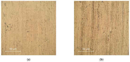
Figure 1.
Pictures of two representative AISI 430 ferritic stainless steel samples with different visual appearances: with a mirror-like finish (a) and with a presence of haze (b). Pictures were taken with a 100× magnification objective, and the field of view was 184.2 μm × 184.2 μm.
The roughness of the samples’ surfaces was analyzed based on the topographic maps obtained by the optical profilometer, as illustrated in Figure 2, following the parameters defined in [23]. It is important to mention that the concept of roughness is relatively ambiguous, insofar as it depends on the scale of interest set by the user. Thus, in [23], a distinction is made between waviness and roughness, and this distinction is made on the application of filters, typically Gaussian, with different cutoff wavelengths, λc.
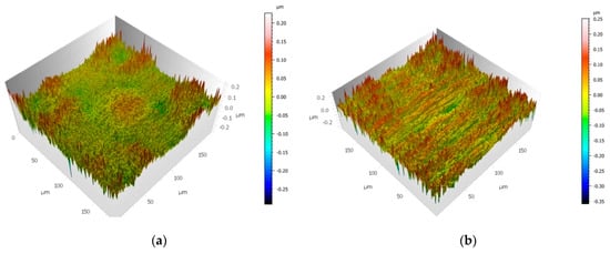
Figure 2.
Three-dimensional topographic maps measured with an optical profilometer for two representative AISI 430 ferritic stainless steel samples with different visual appearances: with a mirror-like finish (a) and with a presence of haze (b).
Primary profiles extracted from the topographic maps of the samples discussed in the previous paragraph have been included as Figure S1 in the Supplementary Material, to illustrate the effect of λc in the discrimination of the low and high spatial frequency height components. It is important to mention that our work is based on the areal method of roughness analysis [23], not on the profile method [26]. However, the workflow to separate high and low spatial frequency components is similar for 1D and 2D topographic records, in such a fashion that the leveling of the height maps is performed on the least square plane of the heights and 2D Gaussian filters are applied to calculate the corresponding areal parameters Sq and Sal, which are shown in Figure 3a,b, respectively, as a function of λc.
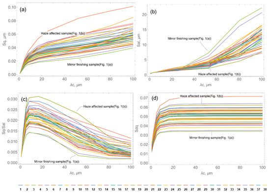
Figure 3.
Values of the roughness parameters as a function of the Gaussian filter cutoff wavelengths determined from the height maps of the AISI 430 ferritic stainless steel samples: root mean square height, Sq (a), autocorrelation length, Sal (b), slope, Sq/Sal (c), and root mean square gradient, Sdq (d). A legend indicating the color of lines representing the various samples is given below the graphs. The colors used for the individual samples are consistent throughout the paper. The curves for the representative samples shown in Figure 1 are marked in the figures for the sake of comparison.
Values for the Sq/Sal ratio were calculated for every λc and are presented in Figure 3c. This ratio is an indicator of the slope of the roughness, but it should not be confused with the root mean square gradient parameter, Sdq, of [23], presented in Figure 3d, which corresponds to the root mean square slope of the heights according to the formula:
Both Sq/Sal and Sdq provide information on the local slope of roughness, which is illustrated in Figure S2 in the Supplementary Material. It is worth mentioning that the slope parameter reported here takes into account the overall effective slope based on the fastest decaying autocorrelation length, Sal.
Finally, the texture aspect ratio, Str, was calculated according to [23] for all the samples. Str takes values in the range 0–1 and is an indicator of the degree of anisotropy of the surface texture (Str = 1 for a completely isotropic surface). Values in the range of 0.05–0.46 were obtained from the primary surfaces of the set of samples under study, which is consistent with anisotropy due to the rolling process.
3.2. Optical Reflection
The representative optical reflection spectra of the samples under study are presented in Figure 4. They were obtained by averaging the set of three spectra taken at different points on each sample’s surface, as described in the Materials and Methods section. The total reflection (diffuse + specular) spectra are shown in Figure 4a and the diffuse reflection spectra are shown in Figure 4b.
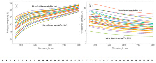
Figure 4.
Optical reflection spectra for the AISI 430 ferritic stainless steel samples, measured with an integrating sphere at total reflection configuration (a), and diffuse reflection configuration (b). The spectra of the samples shown in Figure 1 are marked in the figures for the sake of comparison. A legend indicating the color of lines representing the various samples is given below.
The color coordinates of the surfaces in the color spaces CIE 1931 and CIE 1976 L*a*b* were determined from both the total and diffuse reflection spectra [24,25]. They were calculated for the CIE 1964 10° standard observer, and for both the CIE standard illuminant D65 and the spectral radiance of an LED light source. Particular attention was paid to the luminance coordinate, Y10, which is also known as the light reflectance value (LRV). This is a practical parameter used to quantify the contrast between surfaces, for example, in applications of stainless steel for searching and navigation tasks within buildings [27]. Additionally, attention was paid to the L*, a* and b* color coordinates to quantify any color differences, ΔE*, between the AISI 430 ferritic stainless steel samples under study.
4. Discussion
The results reported here highlight the significant influence of the production process on the surface characteristics of AISI 430 ferritic stainless steel sheet products with a bright finish. This can be observed in Figure 3, where the values of the roughness parameters, Sq and Sal, change significantly from one sample to another, and in Figure 4, where a significant scatter in the optical reflection spectra can be observed, mainly in the diffuse reflection spectra of Figure 4b. Further study into the factors affecting the appearance of bright-finished AISI 430 stainless steel is currently in progress. Differences in grain size do not completely explain the observed differences in reflectivity. It appears to be a complex phenomenon with various originating factors. The results of this study will be reported in due course.
It was found that the total optical reflectance is notably larger than the diffuse optical reflectance in all cases, which indicates that the surfaces are mostly specular, as expected for these materials. It is worth mentioning that similar values for both total and diffuse reflectance have been reported by other authors for AISI 430 stainless steel with a bright finish [28]. However, although at first glance these materials are mostly specular, their surfaces cannot be considered smooth in the sense of the Rayleigh criterion given by Equation (1). If the figures for roughness derived from the non-scale-limited primary surfaces of the samples, such as shown in Figure 2, are taken as inputs for Equation (1), values ranging from 0.389 to 0.997 for θi = 8° and λ = 0.6328 μm are obtained. These values indicate that the diffraction of the scattered light by these samples cannot be approximated as a first-order phenomenon, which would be the case for smooth samples, thus they must be considered rough in the sense of Beckmann–Kirchhoff’s model [11,15,16,17,18,19].
It is not the aim of this work to study the BRDF of these samples, but it is relevant to remember that, in its formulation, the effect of the roughness slope dominates the angular distribution of scattered light on rough surfaces [15,16,29]. The values for the roughness slope parameter, Sq/Sal, are shown in Figure 3c, and a trend can be observed across all the samples under study, with the maximum roughness slope value invariably occurring at a value of λc, within an 8–16.5 μm range. The difference between the values and the behavior for this slope parameter and those observed for the root mean square slope parameter, Sdq, presented in Figure 3d, is noteworthy. As can be seen, the slope parameter, Sq/Sal, shows a greater sensitivity to the cutoff wavelength, λc, than the Sdq slope parameter does, and it highlights more clearly the spatial frequencies involved in the optical reflection of light and, in turn, in the visual appearance of the surface.
We found that the values of the roughness slope parameter, presented in Figure 3c, show a dependence on λc that very plausibly fits the following function:
This fact is illustrated in Figure 5, where the values of Sq/Sal determined for the representative samples of Figure 1 are plotted along with their corresponding fits to Equation (3). Values for the fitting parameters, A and B, for all the samples under study are collated in Table 2. It is worth mentioning that correlation coefficients, r, greater than 0.968 were obtained in all cases.
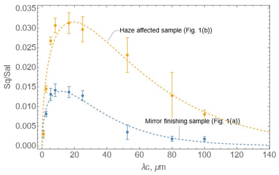
Figure 5.
Fits of the data of slope parameter Sq/Sal vs. λc, to the function of Equation (3), for the two representative samples shown in Figure 1.
Table 2.
Values of the fitting parameters A and B from Equation (3), along with the values of the correlation coefficient r of these fits, as well as the values of the roughness slope parameter calculated according to Equation (4), for the set of AISI 430 ferritic stainless steel samples under study. Samples #18 corresponds to the mirror-finished sample shown in Figure 1a. Sample #25 corresponds to the haze-affected sample shown in Figure 1b.
The influence of the roughness scale in modeling optical scattering has been reported by Marx and Vorburger [30,31], Li and Torrance [17] and Dong et al. [10]. Their findings highlight the importance of spatial bandwidth selection in isolating the roughness scale that dominates scattering behavior. In general, roughness components with small spatial wavelengths diffract light into angles far from the specular direction, and components with long spatial wavelengths diffract light into angles near the specular direction. For this reason, high-pass filtering was performed by [17] and [30], with cutoff wavelengths of 50 μm and in the range of 25–40 μm, respectively, to obtain the roughness surface from the primary surface, whilst low-pass filtering was performed by Dong et al. [10] with a cutoff wavelength of 1 μm, to filter out small-scale roughness, in such a fashion that the surface waviness was obtained from the primary surface.
In the present work, an effective value for roughness slope was calculated from the average value theorem applied to Equation (3), as follows:
where λc0 and λc1 stand for the minimum and maximum values, respectively, of the cutoff wavelengths used, namely, λc0 = 0.0008 μm and λc1 = 0.100 μm. This approach reduces any arbitrariness in filtering, and is effective at balancing the roughness scales involved in visual appearance, as is shown below.
The values of the slope parameter, calculated from Equation (4), were used to analyze the dependence of luminance, Y10, obtained from the diffuse component of the samples’ optical reflection (optical geometry 8°/de), on the surface topography, for both the D65 and the LED illuminants, as illustrated in Figure 6.
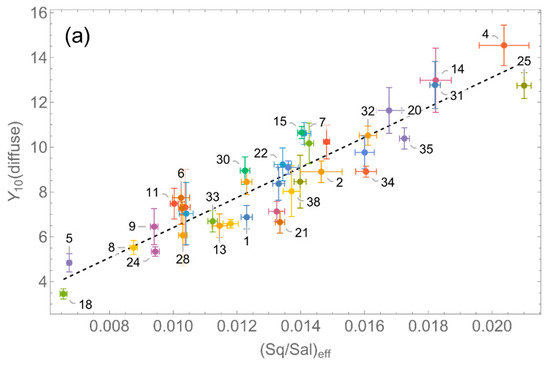
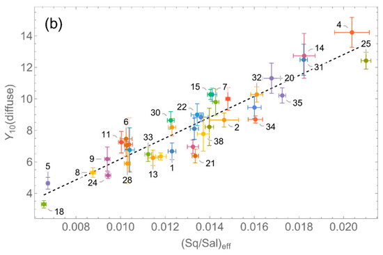
Figure 6.
Values of the luminance coordinate Y10 as a function of the parameter , along with their corresponding linear fits, for the D65 illuminant (a) and an LED light source (b). Values of the r-square correlation coefficient of the fits are 0.925 and 0.927, respectively. Sample IDs from Table 2 have been used in the figures.
A particularly good linear dependence was observed between Y10 and , with correlation coefficient values of r = 0.926 and 0.927, respectively. These results for goodness of fit are very plausible considering the variability observed in the measurements of the reflection spectra and the topography of each sample. It is especially important to note that the linear dependence of luminance, Y10, on the values of Sdq obtained for each λc is, in all cases, notably weaker than the dependence on the effective slope parameter from Equation (4). Correlation coefficients of r < 0.8 have been found for the fits of Y10 vs. Sdq for all values of λc (with r decreasing when the value of λc decreases).
It is worth mentioning that possible metallographic effects that could affect the optical constants of the passive layer cannot be ruled out in the optical reflection results for the samples. However, such effects, if present, do not seem to be exceptionally large nor very scattered, in view of the linear dependence found between the photometric parameter, Y10, and the roughness parameter. Studies on the optical characterization of the passive layer of these samples are currently in progress.
Finally, to complete the study of the visual appearance, the color differences between the AISI 430 ferritic stainless steel samples were analyzed. They were calculated from the samples’ color coordinates in the CIE L*a*b* color space, which were obtained from the total optical reflection spectra (optical geometry 8°/di) and both D65 and LED illuminants. CIE L*a*b* is a perceptually uniform color space, in which numerical differences in the coordinates represent equivalent visual differences, regardless of location within the color space. The coordinates L*, a*, and b* define the distance between two colors by the formula [23,30]:
Equation (5) is the well-known Euclidean distance, and was the original formula used to define the color distance in the CIE L*a*b* color space. Other formulas, such as CIEDE2000, have since been suggested to correct some non-uniformities in the coordinate–perception equivalency [32]. Nevertheless, it was not considered necessary to proceed further in this work for the present study, since our purpose was to highlight differences in the visual appearance of relatively specular non-colored surfaces, rather than to faithfully discriminate between two colored products. Calculations were performed by first determining the centroid of the set of CIE L*a*b* color points for both D65 and LED illuminants, then calculating the distances from the color points to this centroid.
The results, shown in Figure 7, indicate that the distance to the centroid of the set of color points was <8.4 for all the samples in the case of the D65 illuminant, and <3.4 in the case of LED illumination. Taking into account the statistically confirmed ranges for the perception of two colors by a standard observer based on ΔE* [33], namely:
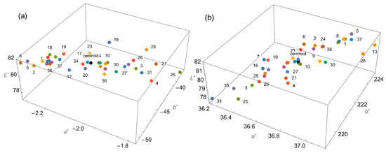
Figure 7.
CIE L*a*b* color coordinates of the AISI 430 ferritic stainless steel samples determined for the D65 illuminant (a) and the LED illuminant (b). The position of the centroid of the set of color points is marked in black. Sample IDs from Table 2 have been used in the figures.
- 0 < ΔE* < 1: the observer does not notice the color difference;
- 1 < ΔE* < 2: only an experienced observer notices the difference;
- 2 < ΔE* < 3.5: an inexperienced observer also notices the difference;
- 3.5 < ΔE* < 5: a clear difference in color is noticed;
- 5 < ΔE*: the observer notices two different colors.
Our results suggest a larger tolerance in color for the AISI 430 ferritic stainless steel products when they are used indoors under LED illumination, compared to outdoors under daylight illumination.
5. Conclusions
The visual appearance of AISI 430 ferritic stainless steel sheet products was analyzed by measuring their surface metrology and photometric properties. The results reported here all clearly indicate that the production process has a strong influence on the surface characteristics of AISI 430 ferritic stainless steel sheet products with a bright finish. Anisotropy was observed in the surface texture; this was found to be consistent with anisotropy related to the rolling process. The surfaces were found to be rough, in the sense of Beckmann–Kirchhoff’s microfacets approach, and the BRDF was found to be strongly dependent on the roughness slope. The spatial filtering of the height maps by Gaussian filters was crucial to limit the roughness scale involved in the diffuse optical reflection. An excellent correlation was found between the photometric luminance, Y10, derived from the diffuse optical reflection, and the scale-limited effective roughness slope parameter proposed in this work. Analysis of the CIE L*a*b* coordinates, which were calculated from the total optical reflection, showed that the color appearance of the AISI 430 ferritic stainless steel products was less significant under LED illumination than under daylight.
Supplementary Materials
The following are available online at https://www.mdpi.com/article/10.3390/met11071058/s1, Figure S1: Sketch illustrating the roughness slope parameter, Figure S2: Height profiles extracted from the 3D topographic maps illustrating the effect of the cut-off wavelength values in the Gaussian filtering.
Author Contributions
Conceptualization, J.M.G.-L.; methodology, J.M.G.-L., E.B. and M.R.d.S.; software, J.M.G.-L.; investigation, J.M.G.-L., E.G., E.B., M.R.d.S., A.N. and J.F.A.; formal analysis, J.M.G.-L., E.B., M.R.d.S., A.N. and J.F.A.; writing—original draft preparation, J.M.G.-L.; writing—review and editing, E.G., E.B., M.R.d.S., A.N. and J.F.A.; funding acquisition, J.M.G.-L. All authors have read and agreed to the published version of the manuscript.
Funding
This work was co-financed by the 2014–2020 ERDF Operational Programme and by the Department of Economy, Knowledge, Business and University of the Regional Government of Andalusia. Project reference: FEDER-UCA18-106321.
Institutional Review Board Statement
Not applicable.
Informed Consent Statement
Not applicable.
Data Availability Statement
Not applicable.
Conflicts of Interest
The authors declare no conflict of interest.
References
- ISO 2813:2014. Paints and Varnishes—Determination of Gloss Value at 20°, 60° and 85°; ISO: Geneva, Switzerland, 2014; Volume 23.
- ASTM. Standard Test Methods for Measurement of Gloss of High-Gloss Surfaces by Abridged Goniophotometry1; American Society for Testing and Materials: West Conshohocken, PA, USA, 2009. [Google Scholar]
- ISO 7668:2018. Anodizing of Aluminium and Its Alloys—Measurement of Specular Reflectance and Specular Gloss of Anodic Oxidation Coatings at Angles of 20 Degrees, 45 Degrees, 60 Degrees or 85 Degrees; ISO: Geneva, Switzerland, 2010.
- ISO 13803:2014. Paints and Varnishes—Determination of Haze on Paint Films at 20 Degrees; International Organization for Standardization: Geneva, Switzerland, 2014.
- ISO 18314-1:2015. Analytical Colorimetry. Part 1: Practical Colour Measurement; International Organization for Standardization: Geneva, Switzerland, 2015.
- Vaidya, S.; Debnath, N.C. Investigation of Physico-Chemical Characteristics of Stainless Steel Surface and Their Effect on the Appearance Aspects of the Alloy Surface. J. Surf. Eng. Mater. Adv. Technol. 2019, 9, 55–87. [Google Scholar] [CrossRef] [Green Version]
- Zhang, Q.; Zhang, B.; Li, R.; Ma, L. Control of surface glossiness during temper rolling aimed at improving visual aesthetics of tinplate. Jixie Gongcheng Xuebao/J. Mech. Eng. 2016, 52, 48–57. [Google Scholar] [CrossRef]
- Harvey, J.E.; Moran, E.C.; Zmek, W.P. Transfer function characterization of grazing incidence optical systems. Appl. Opt. 1988, 27, 1527. [Google Scholar] [CrossRef] [PubMed]
- Donner, C.; Lawrence, J.; Ramamoorthi, R.; Hachisuka, T.; Jensen, H.W.; Nayar, S. An empirical BSSRDF model. ACM Trans. Graph. 2009. [Google Scholar] [CrossRef]
- Dong, Z.; Walter, B.; Marschner, S.; Greenberg, D.P. Predicting appearance from measured microgeometry of metal surfaces. ACM Trans. Graph. 2015, 35. [Google Scholar] [CrossRef]
- Walter, B.; Marschner, S.; Li, H.; Torrance, K. Microfacet models for refraction through rough surfaces. Eurographics 2007, 195–206. [Google Scholar] [CrossRef]
- Cook, R.L.; Torrance, K.E. A Reflectance Model for Computer Graphics. ACM Trans. Graph. 1982, 1, 7–24. [Google Scholar] [CrossRef]
- Frisvad, J.R.; Jensen, S.A.; Madsen, J.S.; Correia, A.; Yang, L.; Gregersen, S.K.S.; Meuret, Y.; Hansen, P.E. Survey of Models for Acquiring the Optical Properties of Translucent Materials. Comput. Graph. Forum 2020, 39, 729–755. [Google Scholar] [CrossRef]
- Rice, S.O. Reflection of electromagnetic waves from slightly rough surfaces. Commun. Pure Appl. Math. 1951, 4, 351–378. [Google Scholar] [CrossRef]
- Stover, J.C. Optical scattering. Meas. Anal. 2012, 9781107003. [Google Scholar] [CrossRef]
- Beckmann, P. Scattering of light by rough surfaces. Prog. Opt. 1967, 6, 53–69. [Google Scholar] [CrossRef]
- Li, H.; Torrance, K.E. An Experimental Study of the Correlation between Surface Roughness and Light Scattering for Rough Metallic Surfaces. In Advanced Characterization Techniques for Optics, Semiconductors, and Nanotechnologies II; SPIE: Bellingham, WA, USA, 2005; p. 58780V. [Google Scholar]
- Torrance, K.E.; Sparrow, E.M. Theory for off-specular reflection from roughened surfaces. J. Opt. Soc. Am. 1967, 57, 1105. [Google Scholar] [CrossRef]
- He, X.D.; Torrance, K.E.; Sillion, F.X.; Greenberg, D.P. A comprehensive physical model for light reflection. Proceedings of the 18th Annual Conference on Computer Graphics and Interactive Techniques. Siggraph 1991, 25, 175–186. [Google Scholar] [CrossRef]
- García, I.C.; Galindo, A.N.; Almagro Bello, J.F.; González Leal, J.M.; Botana Pedemonte, J.F. Characterisation of high temperature oxidation phenomena during AISI 430 stainless steel manufacturing under a controlled H2 atmosphere for bright annealing. Metals 2021, 11, 191. [Google Scholar] [CrossRef]
- EN 10088-2:2014. Stainless Steels. Part 2: Technical Delivery Conditions for Sheet/Plate and Strip of Corrosion Resisting Steels for General Purposes; European Committee for Standardization Comité: Brussels, Belgium, 2015.
- ASTM E112. Standard Test Methods for Determining Average Grain Size E112-10; ASTM E112-10; ASTM: West Conshohocken, PA, USA, 2010; Volume 96, pp. 1–27. [CrossRef]
- ISO 25178-2:2012. Geometrical Product Specifications (GPS)—Surface Texture: Areal—Part 2: Terms, Definitions and Surface Texture Parameters; International Organization for Standardization: Geneva, Switzerland, 2012.
- CIE 130:1998. Practical Methods for the Measurement of Reflectance and Transmittance; International Commission on Illumination: Vienna, Austria, 1998.
- CIE 15:2004. Technical Report: Colorimetry, 3rd ed.; International Commission on Illumination: Vienna, Austria, 2004.
- ISO 4287:1997. Geometrical Product Specifications (GPS)—Surface Texture: Profile Method—Terms, Definitions and Surface Texture Parameters; International Organization for Standardization: Geneva, Switzerland, 2015.
- BS 8493:2008+A1:2010. Light Reflectance Value (LRV) of a Surface—Method of Test; British Standard Institution: London, UK, 2010.
- Lee, S.J.; Chen, Y.H.; Liu, C.P.; Fan, T.J. Electrochemical mechanical polishing of flexible stainless steel substrate for thin-film solar cells. Int. J. Electrochem. Sci. 2013, 8, 6878–6888. [Google Scholar]
- Yang, Y.; Buckius, R.O. Surface length scale contributions to the directional and hemispherical emissivity and reflectivity. J. Thermophys. Heat Transf. 1995, 9, 653–659. [Google Scholar] [CrossRef]
- Marx, E.; Vorburger, T.V. Direct and inverse problems for light scattered by rough surfaces. Appl. Opt. 1990, 29, 3613. [Google Scholar] [CrossRef] [PubMed]
- Vorburger, T.V.; Marx, E.; Lettieri, T.R. Regimes of surface roughness measurable with light scattering. Appl. Opt. 1993, 32, 3401. [Google Scholar] [CrossRef]
- CIE 142:2001. Improvement to Industrial Colour-Difference Evaluation; International Commission on Illumination: Vienna, Austria, 2001.
- Mokrzycki, W.; Tatol, M. Color difference Delta E—A survey Colour difference ∆ E—A survey Faculty of Mathematics and Informatics. Mach. Graph. Vis. 2011, 20, 383–411. [Google Scholar]
Publisher’s Note: MDPI stays neutral with regard to jurisdictional claims in published maps and institutional affiliations. |
© 2021 by the authors. Licensee MDPI, Basel, Switzerland. This article is an open access article distributed under the terms and conditions of the Creative Commons Attribution (CC BY) license (https://creativecommons.org/licenses/by/4.0/).