1. Introduction
By following the classic definition in information theory, entropy represents a measure of the ignorance of the target system under investigation [
1]. This is generally utilized to define its intrinsic complexity, i.e., non-uniformity. Its application for structural health monitoring (SHM) purposes stems from a conjecture of a possible eighth axiom of SHM, as reported in Farrar et al. [
2] a decade ago:
“The presence of damage in a structure or system usually results in increased complexity of measured responses or features”.
In other words, the concept is that damage can be detected and assessed through statistics and signal processing as a time- and space-defined variation in the system’s structural complexity, as further detailed more recently in [
3].
The SHM axioms [
2,
4] aimed to provide a framework for the principled selection of effective damage-sensitive features (DSFs). In this regard, entropy is widely considered the measure of diversity/complexity par excellence. For instance, the Shannon entropy has been proved to be equivalent to the true diversity index with a Hill number of unit order
[
5]. Therefore, it makes sense to apply entropy measurements as a DSF.
Some entropy-based SHM approaches reported in the last years in the scientific literature include the use of power spectral entropy [
6] and multiscale cross-sample entropy [
7]. In [
8], the authors proposed an interesting interpretation of the insurgence and development of fatigue, corrosion, wear, radiation, and creep damage as irreversible thermodynamics phenomena, thus from an entropic point of view.
Recently, in [
9] benchmarked Shannon, Rényi, permutation, sample, approximate, and spectral entropy for SHM purposes. The authors of [
10] performed a similar comparison between Wiener and Shannon spectral entropy for the application to mixed brick-stone masonry structures, considering experimental evidence from three case studies damaged from previous seismic events.
Indeed, the basic principles of the procedure reported here were set in [
10,
11]. In the present paper, these principles are expanded, further detailed, and validated on a numerically simulated case study of a buried steel pipe. This application, relevant in the context of oil & gas engineering, presents several differences in comparison with the masonry buildings analyzed in [
10,
11]. Underground structures are inherently challenging due to:
- (1)
The impossibility to directly excite the structure with a controlled input; and
- (2)
The very stiff boundary conditions.
These aspects are shared by many geotechnical applications, such as deep foundation piles, which are very difficult to investigate for structural integrity [
12,
13]. This is mainly due to the very small amplitude of the output displacements, naturally induced by ambient vibrations (AVs) and recorded with a grid of sensing devices. In fact, it is notoriously difficult to extract reliable DSFs from output-only recordings from weakly-excited structures (see, e.g., a case study for cultural heritage preservation in [
14]). As will be shown here, entropy measures are instead particularly well-suited for dealing with low-amplitude, random signals.
In this work, the potentialities of this framework were methodically investigated for the first 2/3 main tasks of SHM, defined according to the classic Rytter’s hierarchy [
15,
16].
The remainder of this paper is organized as follows:
Section 2 describes the theoretical framework of the proposed approach; in
Section 3, the context of this application is briefly outlined; the numerical case study is detailed in
Section 4; the results are discussed in the following
Section 5; and
Section 6 (Conclusions) ends this paper.
2. Wiener Entropy Measurements for SHM Purposes
Out of the several definitions of ‘entropy’ currently reported in the scientific literature, the Wiener entropy (WE, also known as spectral flatness) was found to be particularly well-suited for metallic structures in previous studies [
17]. The main motivation resides in its greater sensitivity to small alterations in comparison to the more common Shannon spectral entropy. This is relatively inconvenient for masonry or concrete structures, where the material inhomogeneity and variability may cause damage-unrelated fluctuations. In turn, these cause a higher risk of false-positive identifications [
10], which are a common threat to vibration-based SHM [
18]. On the other hand, for more homogeneous building materials, this greater accuracy can instead be exploited to detect small cracks in their earlier extension phases.
The WE can be mathematically defined in a discretized fashion as:
where
B represents the total number of frequency bins, that is to say, the number of discrete measurements in the frequency domain, while
is the (discretized) power spectrum of the recorded vibrational time history, evaluated at frequency
.
The convenience of entropy measurements over other, more classic, approaches directly derives from the specific conditions of underground pipeline monitoring.
The first aspect regards the amplitude of the system input and output. As hinted above, the AV input is very low, and thus the system is only weakly excited. Due to this minimal excitation level and the increased stiffness from the confining soil, the expected output amplitude is even lower in amplitude. Generally, this is an inconvenient condition.
One can consider the following: the system behaves more deterministically for increasing input energy. In fact, the energy of the system’s response is naturally amplified more at the natural frequencies than at other frequencies. Thus, increasing the system energy increases this disproportion and, therefore, inherently reduces the flatness of the frequency spectrum. In contrast, at low energy levels, the actual response tend to become indistinguishable from the measurement noise, the system behaves mostly non-deterministically, and the responses will have inherently higher entropy.
The second aspect regards the frequency content of the input. For system identification (SI) purposes, it is preferable to have a controlled input in order to excite only specific portions of the system’s global dynamics. This is, e.g., the case of chirp or stepped sines, which allow to isolate and follow a specific resonance frequency even in nonlinear conditions. However, the Gaussianity of ambient dynamic loads (due to the central limit theorem) guarantees an (almost) flat distribution of energy in the frequency domain, which is ideal for entropy measurements [
19].
Thus, these two aspects—the natural spectral flatness of the input signal and the very low amplitude of the output response—make the use of the Wiener entropy/spectral flatness particularly well-suited for buried metallic structures.
The rest of this discussion aims to verify the use of entropy measurements as a health state indicator for the several tasks included in a complete SHM diagnosis. These include, according to the classic hierarchical structure proposed by Rytter [
15]:
(single- or multi-) Damage Detection: to identify if one or more damage(s) are present or not in the structure;
(single- or multi-) Damage Localization: to define the most probable position of damage;
(single- or multi-) Damage Assessment: to evaluate the severity of the damage(s);
(single- or multi-) Damage Prediction: to establish the expected future growth of damage.
The last step is of less interest here since it will require further statistical information concerning the expected remaining useful life (e.g., prognosis).
2.1. Uses for Damage Detection
The values of WE can be computed at any point and compared with the known baseline computed from the pristine system. This approach is in accordance with the classic statistical framework of pattern recognition-based SHM [
20].
However, a deviation from the normality model is not necessarily an indicator of damage per se. Such deviations could happen due to damage-unrelated confounding influences, collectively known as environmental and operational variations (EOVs, [
21,
22]). For this reason, the pipeline is here investigated only without any internal pressure to avoid changes in the stress field induced by the changing operating conditions. The rationale is that SHM is rarely performed online and in real-time but rather periodically, during a phase of inactivity (e.g., at night, see for instance [
23]). For unchanged external conditions, any statistically relevant variation can be then pinpointed to a change in the internal structure of the target system, i.e., to damage.
2.2. Uses for Damage Localisation
The effects of damage fade moving away from its location. This represents a limitation for single-output damage detection, since the acquisition channel may be too far from the damage to detect it correctly. However, with a properly placed array of sensors (thus, with a multi-output acquisition system), this spatial variability can be exploited to locate the (single or multiple) source(s) of inconsistency.
2.3. Uses for Damage Severity Assessment
The physical, quantitative assessment of the damage severity would require some a priori knowledge about the expected damage effects. This is not considered here as the proposed framework is based only on data from the undamaged conditions of the target system. Nevertheless, it is still possible to qualitatively estimate the severity of damage by comparing the divergence between the WE values estimated from pre-and post-damage recordings.
3. Buried Oil & Gas Pipelines
Pipelines are defined by four main factors: their external environment (i.e., the boundary conditions), construction material, diameter, and thickness.
Regarding the external environment, buried pipelines are the predilected alternative for the distribution of liquid resources over long distances. On the one hand, this is particularly convenient to avoid interferences with other infrastructures, especially in proximity of urbanized areas and potential incidents. Following the terminology in [
24], ‘incidents’ refers in this context to both nonintentional accidents and sabotage or terroristic events. On the other hand, this choice makes visual inspection—which still is the most common practice for scheduled maintenance—unfeasible. This is even more evident for subsea pipelines, which stretch below the seabed inside purposely excavated trenches. Anyhow, even if doable, the length and ramifications of pipeline networks make man-made visual inspection generally not cost-efficient. Thus, automated and vibration-based approaches are preferable.
The reliability of such structural health monitoring (SHM) systems is nevertheless of paramount importance due to the deleterious consequence of damage. This might result in the leakage of pressurized inflammable liquids, with the potential for fire and explosion. The costs in terms of human losses, disruption to the energy supply network, environmental pollution, and other geohazards make the research into advanced solutions economically convenient. Their sensitivity is relevant as well; in high-stress lines, even small cracks can rapidly grow due to the spilling of highly pressurized fluids and lead to abrupt rupture [
25].
For these underground uses, two main categories of pipes are generally employed: “rigid” and “flexible” pipelines. The former group is made up of the so-called pre-stressed concrete cylinder pipes (PCCP), while the latter one consists of metallic structures. The mechanical behavior is very different in these two options, as in PCCPs the pipe structure carries the structural loads itself, while in steel pipes (SPs) they are supported by the soil-structure interactions, thanks to the steel capability to deflect without breaking.
This discussion will focus on SPs, since they are overwhelmingly more widespread for oil & gas transportations, both on- and offshore. For the industry needs, oil, gas, and/or pressurized natural gas liquids (NGLs) are moved through these pipelines thanks to compressor (for gas lines) or pump (for oil and NGLs) stations departing from the production regions to distribution centers. In this sense, they represent a much more economically convenient and safer way of transportation than by rail or road [
26], with statistics reporting only two deaths and 11 injuries on average per year between 1999 and 2001 on US territory, compared to the several thousand involved in truck crashes in the same period [
27].
SPs are generally made in carbon steel due to this material’s strength, relatively low weight, and ease of workability. Alloy steels are also applied frequently; alloying elements generally improve mechanical resistance but at a major economic cost, and thus they are reserved for specific uses at extremely high temperatures and pressure. The interested reader is referred to [
28] for other relevant aspects about the design and structural analysis of buried flexible steel pipelines.
3.1. Typical Damages and Defects
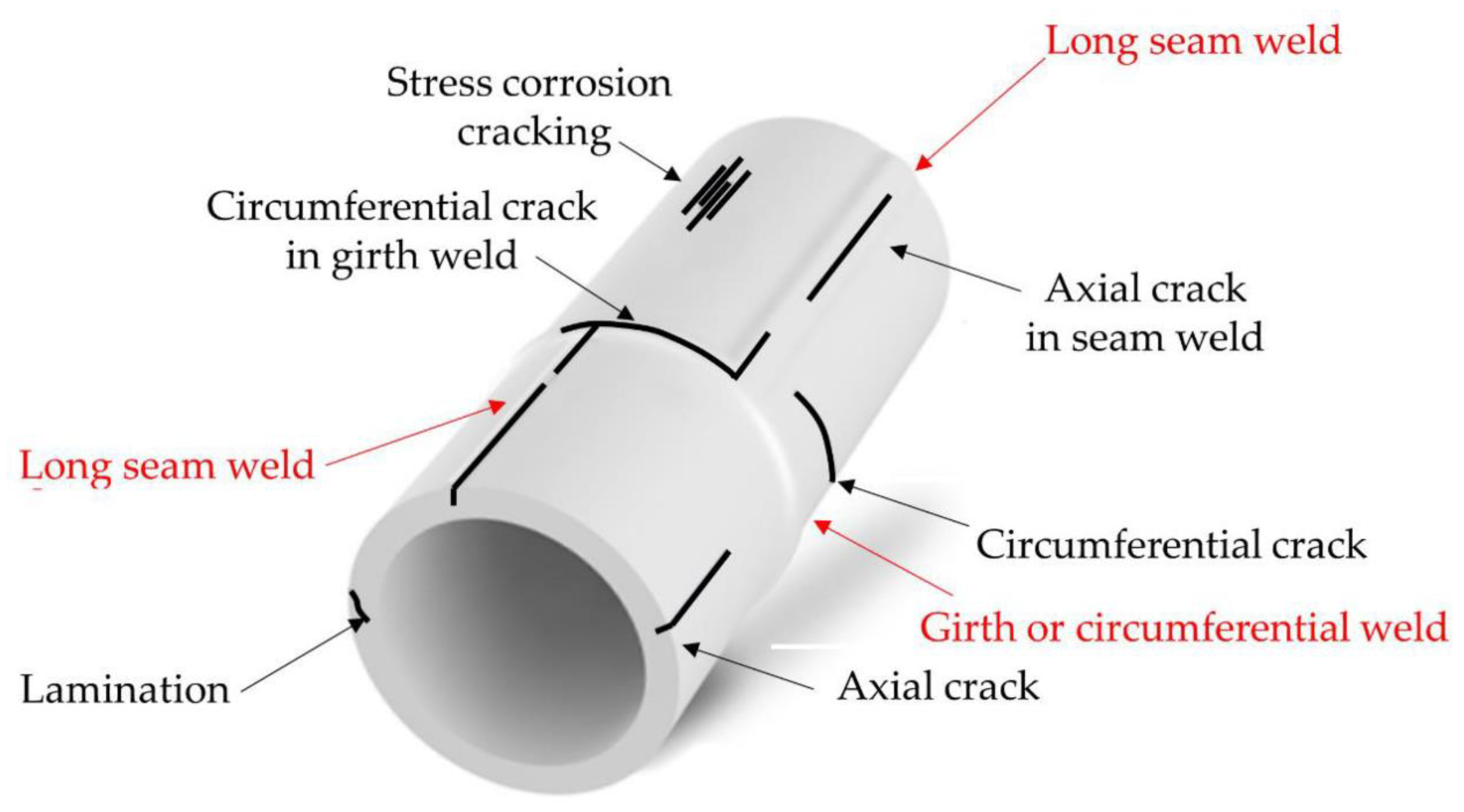
A geometry-based classification of main damage typologies frequently encountered in buried pipelines can be found in [
29]. These include several crack shapes (circumferential, longitudinal, spiral, or others), plus blowout holes. Some examples are represented in
Figure 1.
The most commonly occurring types of damage can be further classified according to the different failure mechanisms from which they originate. These typically include pitting corrosion, pipeline thinning, and pipe bursts. These latter ones are caused by sudden transient pressures of the carried liquid (e.g., the “water hammer” phenomenon). The pipeline thinning, generally, derives from steel corrosion, graphitization, or other material-related degradation phenomena which result in metal loss. These are all time-dependent and intensified by the exposition to a chemically aggressive environment, both externally (i.e., in the surrounding soil) and/or internally (i.e., in the transported fluid).
Apart from mechanical fatigue and corrosion, other damaging factors include manufacturing-related defects, which are known to cause internal cavities which coalesce into larger cracks under mechanical stress [
30], and defective welding. This latter case may result in localized damages or larger coupling failures. Rapid (e.g., landslides) or slow (e.g., long-term subsidence) large land movements of the nearby and underneath soil are two other frequent issues, as well as weather-related and natural phenomena. Due to their long extension, pipelines are also strongly vulnerable to seismic events and other large natural disasters (this aspect is analyzed in-depth in [
31]).
Finally, mechanical damages (voluntary or involuntary, such as vandalism, impacts, incorrect operations) constitute a significant cause of instantaneous, immediate failure. Mechanical damages caused by third-party excavation are widely considered as the main cause of pipeline failure.
In their less severe form, these generally result in dent and gouge defects. More rarely, these may cause latent weak points, very difficult to detect due to their limited area and severity, until they lead to rapid collapse even after years.
Plain dents, which may occur due to small ground movements, rock impingement, poor installation, or limited buckling phenomena, are not of great interest here since they usually are not harmful, provided they are not excessively large [
32]. Thus, they have not been considered for this study.
For the sake of this study, two different typologies of damage have been considered and numerically modeled. In the first case, localized reductions in the material stiffness are representative of dents or manufacturing defects (for low damage severity), pitting corrosion (at intermediate/high damage level), or any through-thickness crack (for higher damage intensity). In the second case, the stiffness is uniformly reduced over a narrow ring-like cross-section of the pipe. This is intended to replicate, e.g., the loosening of bolts at joints. More details about the modelling of these two damage cases will be provided throughout
Section 4.
3.2. Typical Approaches for Pipeline Monitoring
There are several best practices reported in the scientific literature regarding pipeline integrity management (PIM; see, e.g., [
33]). These can be categorized between maintenance surveys, which can potentially include some non-destructive testing (NDT) techniques, and long-term SHM apparatuses, which apply embedded sensors. Techniques and approaches for both categories have been extensively reviewed, e.g., in [
34,
35].
Regarding NDTs, some approaches worthy of note include ultrasonic techniques (reviewed by [
36]), acoustic emissions (AE, [
37]), eddy currents, etc. These point-wise, localized approaches require, however, a nearby (robotic or human) operator. In this sense, for scheduled maintenance and surveys, the use of instrumented pipeline inspection gauge (PIG) [
38] represents one of the main options for unmanned inspections to date. However, pipelines dedicated to the transportations of explosive fluids are generally deemed as “unpiggable” due to safety reasons. For these and other reasons, man- or robot-made periodical inspections are not cost-efficient. Thus, output-only, vibration-based approaches are preferable from a practical and economical point of view.
The procedure proposed in this work falls in this latter group, utilizing optical fibers deployed along the pipe length for strain measurements. In this regard, a concise yet quite complete review of sensors for vibration-based and non-vibrational SHM in buried pipes can be found in [
39] (the specific application is for underground water supply systems, but the differences are irrelevant for what concerns the sensing technologies).
4. The Finite Element Models
In this research, two sets of finite elements (FE) were considered. Both sets were made up of a pristine SP and its damaged counterparts.
Firstly, to better investigate the feature (Wiener entropy of axial strains) performance, all unnecessary sources of uncertainties—such as material inhomogeneities—were omitted in this first set of tests. Measurement noise was artificially added to corrupt the signals.
On the other hand, initial flaws on the SP and uneven distribution of the soil material properties in the surrounding areas were included in the second case (being already included in the first model the non-uniform distribution of the soil stiffness due to the location of the pipeline in the depth). This point will be better addressed later in a dedicated Section.
All the FE models were built on Ansys
® Mechanical APDL™. Here in this section, only the first model will be discussed in detail. The differences between the first and the second numerical case study will be detailed in the dedicated
Section 6.
The structure consists of a 20 m-long section of steel pipeline. The SP was realized with 4-node, 6-DoFs-per-node finite elements. Linear-elastic spring-like elements were used to simulate the presence of the surrounding soil in the three directions (see
Figure 2). Each spring has a different stiffness value depending on the model geometry. The specific details of this modeling choice will be discussed in the next subsections.
The mass participation of the soil was considered with an additional term in the SP density by minimizing the difference between the fundamental natural frequency of the plane strain model of soil and SP (
Figure 2b) and the fundamental natural frequency of a local model of the SP surrounded by springs (
Figure 2c) with stiffness obtained by the FE model of the soil.
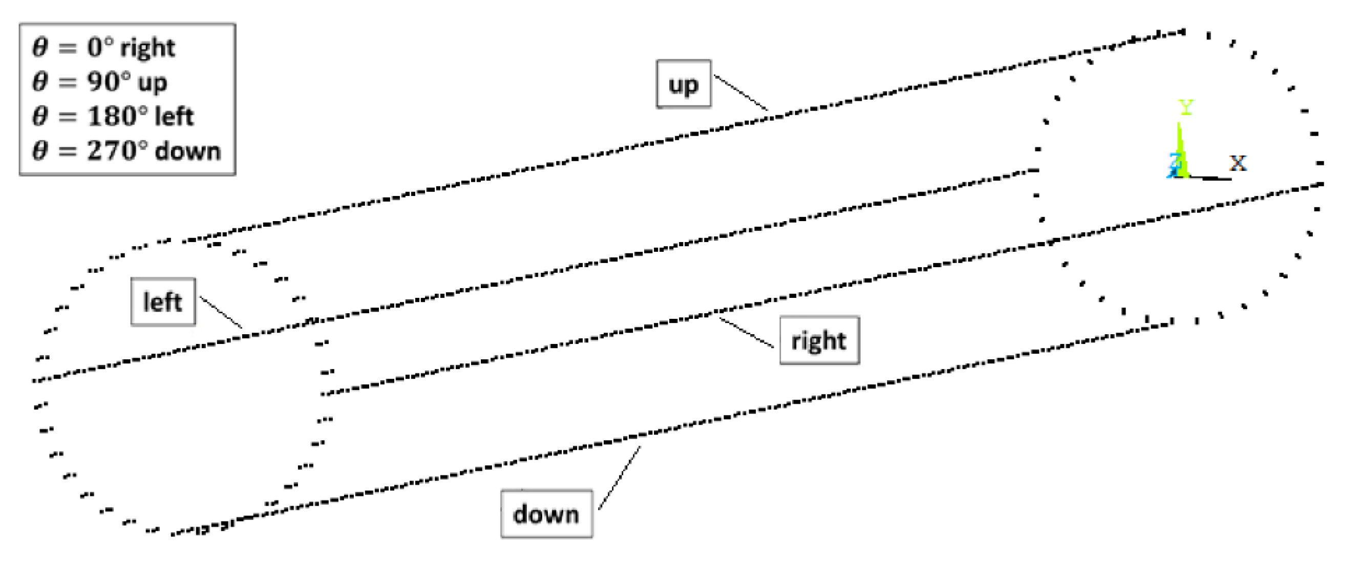
The global reference system was located at the centroid of the SP on one end, with the z-axis oriented along the main pipe axis, the y-axis perfectly vertical and pointing upward, and the x-axis perfectly horizontal to form a right-handed triad. The stiffness of the springs in the z-direction was assumed to equal the one in the horizontal direction. This multi-modeling approach was needed to consider the effect of the soil in the dynamics of the SP in an way needing less computational effort, allowing the simulation of several damage scenarios.
4.1. Cross-Sectional Geometry of the Pipe
The geometry of the pipeline cross-section was designed as follows. A relatively large diameter (100 cm) was considered. The choice was made considering that the nominal diameter for underground subsea pipelines generally ranges from a minimum diameter of 6″ (~15.2 cm) to a maximum of 48″ (~121.9 cm) [
40]. The uniform thickness was thus computed according to ASME code B31.3, considering an allowable tensile stress equal to 16,000 psi (110.32 MPa), quality factor for piping material equal to 0.8, wall thickness coefficient equal to 0.4. To simulate operating conditions, a liquid pressure of about 600 psi wwas assumed, i.e., ~4.14 MPa. This resulted in 22 mm-thick walls. Thus, the pipeline cross-section is defined by an inner diameter of 98.9 cm and an outer diameter of 101.1 cm, with a uniform thickness. The pipe centroid was located at −200 cm (below ground level) for all cross-sections. A consistent mass matrix was applied.
4.2. Material Properties
The parameters of standard carbon steel type 235 have been considered for the construction material (see the second column of
Table 1), as retrieved from [
41] and following the current European regulations [
42]. Type 235 is commonly used in piping systems with minimum design temperature ≥−15 °C and pipe thickness <3 cm [
43]. A linear elastic behavior was assumed for the steel; this assumption is justified by the small strains during operating conditions.
4.3. Boundary Conditions and Soil-Structure Interactions
The boundary conditions for the steel pipeline can be divided between the internal and the external boundaries. On the inside, the pipeline was assumed to be empty and have no internal pressure due to the reasons discussed in
Section 2.1.
Concerning the soil-structure interactions, the following assumptions have been made:
- −
The mass and stiffening effects of the surrounding soil volume are emulated by a set of spring elements;
- −
The SP boundaries are connected to these springs, and the edges of the springs opposite to those connected to the SP are fully restrained, i.e., they do not vibrate independently;
- −
The random noise forces transmitted by the surrounding soil are directly applied on the SP external edge;
- −
A Rayleigh damping model is assumed, with mass and stiffness multipliers equal to 2.954362 and 0.000304, respectively, which corresponds to 3% damping ratio on the first two modes of the SP.
Indeed, the FE model aimed to reproduce the soil effects in a realistic yet simplified way without explicitly modeling the ground surrounding the pipeline. The rationale, as introduced before, was that the focus of this research was on the structural, and not geotechnical, vibrational response of the model. To this goal, a set of properly calibrated springs can effectively reproduce the static and dynamic soil-structure interactions (SSIs) of underground structures (see e.g., [
44] for an example of a wind turbine mono-pile foundation). Specifically, 21,600 spring elements were utilized.
The stiffness coefficients of the springs were obtained by static analyzing a dedicated plane strain model of the soil surrounding the SP. Specifically, the spring calibration procedure followed four modeling phases:
- (1)
The whole soil was modeled with 4-node, 2-DoFs-per-node plane elements (as can be seen in
Figure 2a), considering a cylindric volume of radius
and centered on the pipeline centroid. To avoid edge effects,
R was increased until
m, which was found to be large enough to eliminate any effect of the external boundaries at the soil-structure interface. This procedure followed the current standard practices in the geotechnical analysis of ground excavations. Values of
caused the strain field close to the pipe hole to be biased from boundary conditions. Clean sand was assumed for the soil, with a single layer for the whole volume and linear elastic behavior. The mechanical parameters, retrieved from [
41], were: density 1850 kg/m
3, Young’s modulus 24 MPa, and Poisson’s ratio 0.20. No water table was considered. The external boundaries of the soil volume were defined with no external loads or constraints applied on the flat, perfectly horizontal ground surface. Fixed (zero displacements) constraints were set on the remaining sides. This model was used to define the stiffness of the soil affecting the response of the SP, which has been modeled with independent springs in the third and fourth FE models.
- (2)
The second model is identical to the first, except for the presence of the SP (
Figure 2b)
- (3)
The third (yet plane) model added to the SP the presence of the springs. Together with the second FE model, this model was used to calibrate the mass participation of the soil to the dynamics of the soil-SP system.
- (4)
Finally, the fourth reference, the FE model, is constituted by a 3D representation of the pipelines (20 m long), which was modeled with shell elements. A series of springs, calibrated in the previous steps, were used to simulate the contribution of the soil to the dynamics of the soil-SP system in the 3 spatial directions effortlessly.
4.4. Input Definition and Simulation Settings
The AVs are generally classified as microseismicity, induced by natural sources, predominantly between the 0~1 Hz range, and microtremors, generated by nearby human activities such as pedestrian, traffic, and machinery [
45]. These latter ones cover the higher frequencies (1 to 10
20 Hz) and are more subject to intra- and inter-day variability [
46].
For the former group, for regions not too far inland, as in the Italian peninsula, the main natural phenomena originating the natural AVs are the waves impacting the coast (in the range 0.05–0.1 Hz according to [
47], 0.5–1.2 Hz according to [
48]), large scale meteorological perturbation on site (0.1–0.25 Hz [
47], 0.16–0.5 Hz [
48]), and large scale meteorological events on nearby seas/oceans (0.3–1 Hz [
47], 0.5–3 Hz [
48]). However, the current expert consensus indicates the range of engineering interest between 0.5 and 20 Hz [
49], i.e., the frequency range is mainly affected by anthropic activities [
50]. Thus, the following assumptions and considerations have been made:
The AVs are applied as independent point-like sources of white Gaussian noise (WGN) time histories of forces;
The AVs are applied at each node of the boundaries of the SP;
The frequency and amplitude content of the AVs is stationary (i.e., not time-dependent);
In each direction, the WGN is assumed with zero mean and unit variance;
At each point-like source, the AVs are applied in the three main directions (x-, y-, and z-axes).
Concerning the first assumption, the Gaussian distribution of independent random point-like sources is derived from the state of the art in AV numerical modeling [
49].
The application of the forces on the edges of the SP is intended to mimic the random vibration of the surrounding soil.
Concerning the third assumption, it is assumed that the measurements are performed in absence of abrupt variations during recording. This is assured for the small portion of microseismic noise in these interferences. Even for the larger anthropogenic portion, this is reasonable due to its slow variation rate, generally corresponding to the day/night and seasonal cycles (as experimentally validated in [
23]). These timescales are much larger than the average acquisition duration.
Concerning the amount of variance of the external force, it is worth stating that its definition is arbitrary and does not affect the results of the proposed approach.
Indeed, it is well known that the standard deviation of a linear transformation Y (with zero intercepts) of a random variable X, i.e., Y = kX (with k constant of proportionality) is proportional to the standard deviation of the reference random variable X, i.e., (in the present work, X is a Gaussian distribution with unit variance or standard deviation, i.e., , and ).
Thus, being a linear model, the structural response will vary linearly for a uniform linear variation of the external force vector
x. In this case, the external force vector is made up of the realization of the random variable
X. Then, since (i) the Fourier Transform is a linear operator, and thus:
where
and
are generic power spectra of the components of
r and
u (with
r and
u two generic proportional response displacement fields) and since (ii) the WE is scale-invariant, i.e.,:
Thus, for any value of the chosen variance or standard deviation of the external force vector x, the WE will remain unchanged.
Therefore, a transient dynamic analysis was performed on the baseline (undamaged) model and for all the investigated damage scenarios (see
Section 4.6) for a total duration of 20 + 20 s (to obtain a frequency resolution of
Hz). The readings at the 800 output channels were sampled at
fs = 1000 Hz.
The resulting time series of axial strains have been then artificially corrupted by adding Gaussian noise with zero mean and standard deviation proportional to the standard deviation of the uncorrupted output signals. This is intended to simulate measurement noise during acquisition. Specifically, the robustness to noise has been addressed by considering three levels of noise to signal ratio (NSR) (in terms of noise and signal standard deviation): 0% (ideally noise-free), 5%, and 10%.
4.5. Simulated Sensor Layout
The pipeline is assumed to be instrumented with a set of four optic fibers arranged as depicted in
Figure 3. This is compatible with state of the art practices in the field; e.g., a system of distributed fiber optic sensors was used, e.g., in [
51] to perform strain measurements. The four optic fibers are labeled according to their angular coordinate, as expressed in the legend of
Figure 2. We considered 200 measurement points per fiber, totaling 800 output channels. These were equally spaced from each other by steps of
m along a 20 m-long tract of the pipeline length. To emulate the readings from Fiber Bragg grating (FBG) sensors [
52], the axial strains (along the z-direction in the model) were considered as the quantity of interest.
4.6. Damaged FE Models
Considering the two typologies of damage described in
Section 3.1, the occurrence of damage was simulated by reducing the stiffness in specific elements of the FE model. This is a classic model choice [
53], frequently applied also in geometrically complex models [
54]. The location of the damaged area is described in
Table 2 and graphically portrayed in
Figure 4.
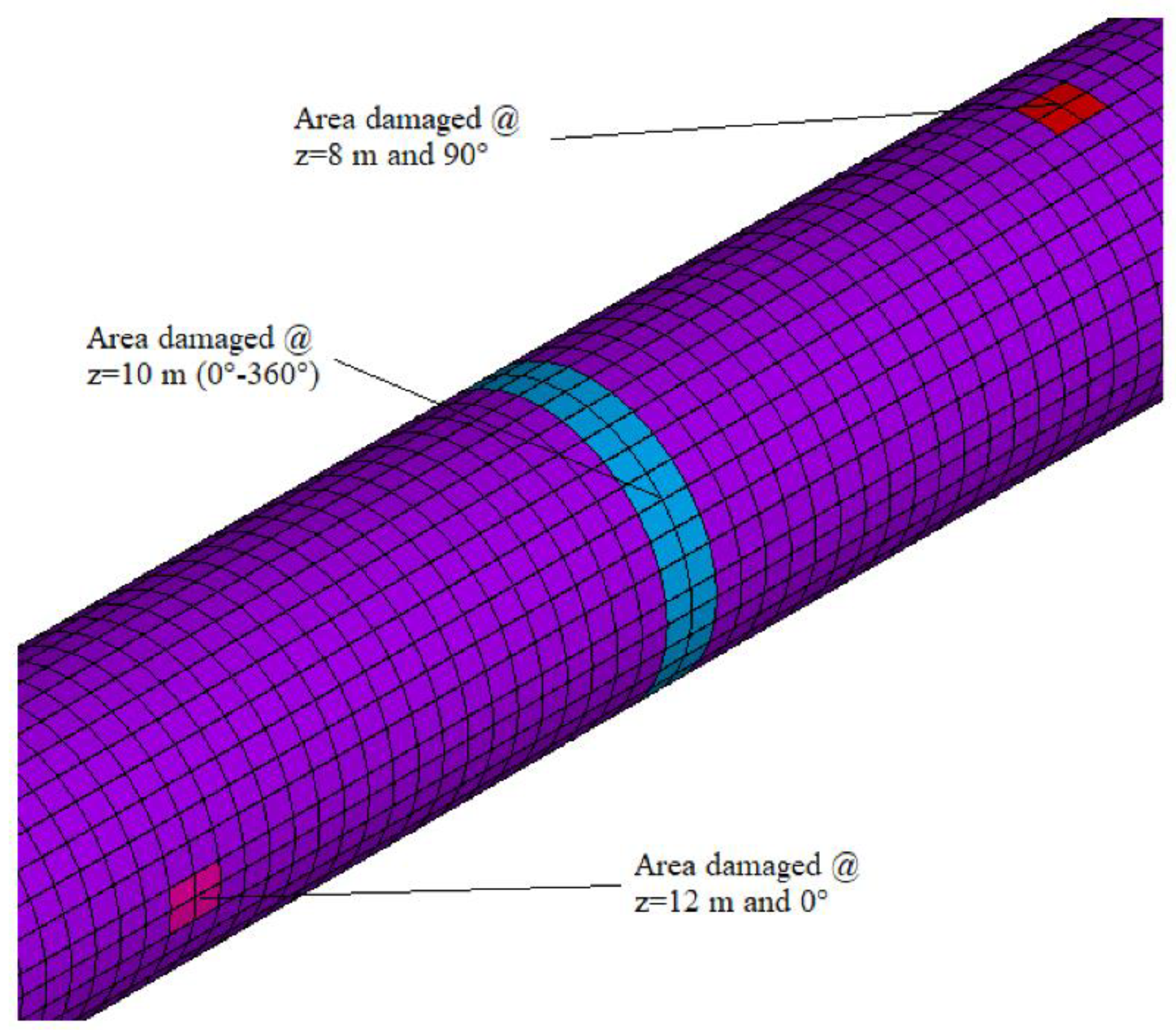
In
Table 2,
zc and
θc represent the cylindrical coordinates of the centroid for the damaged area (the damage extends symmetrically from it along both
z and
θ). C indicates the pipeline circumference (3.14 m). Damages #1 and #3 occupy an area of 0.0314 m
2, encompassing about 5% of the whole circumference. These are intended to represent localized damages, which are inherently more difficult to defect. For the same damage length along the
z-axis, damage #2 covers 100% C, resulting in a much larger surface (0.628 m
2). This second typology can be seen as both a weakened or degraded girth weld or a loose bolted joint.
Several combinations of damage intensity levels have been considered. From hereinafter, these will be indicated by their percentage of reduction with respect to the pristine Young’s modulus. For instance, 80%/20%/0% will indicate an 80% reduction for damage #1, 20% for damage #2, and no damage at θc = 0° and zc = 12 m. Damage growth was emulated as well, increasing step-by-step the damage intensity in the selected areas. This procedure mimics the natural progression of damage, even if at a discrete pace.
5. Results
To demonstrate the WE variations at different damage states (location and severity), the following health state indicator was assumed:
where
is the reference, initial, WE measured over the system, while
is the WE at a generic structural state. The results of the numerical simulations were addressed in light of the classic Rytter’s hierarchy, considering both basic (damage detection) and more advanced (damage localization and severity assessment) tasks for SHM.
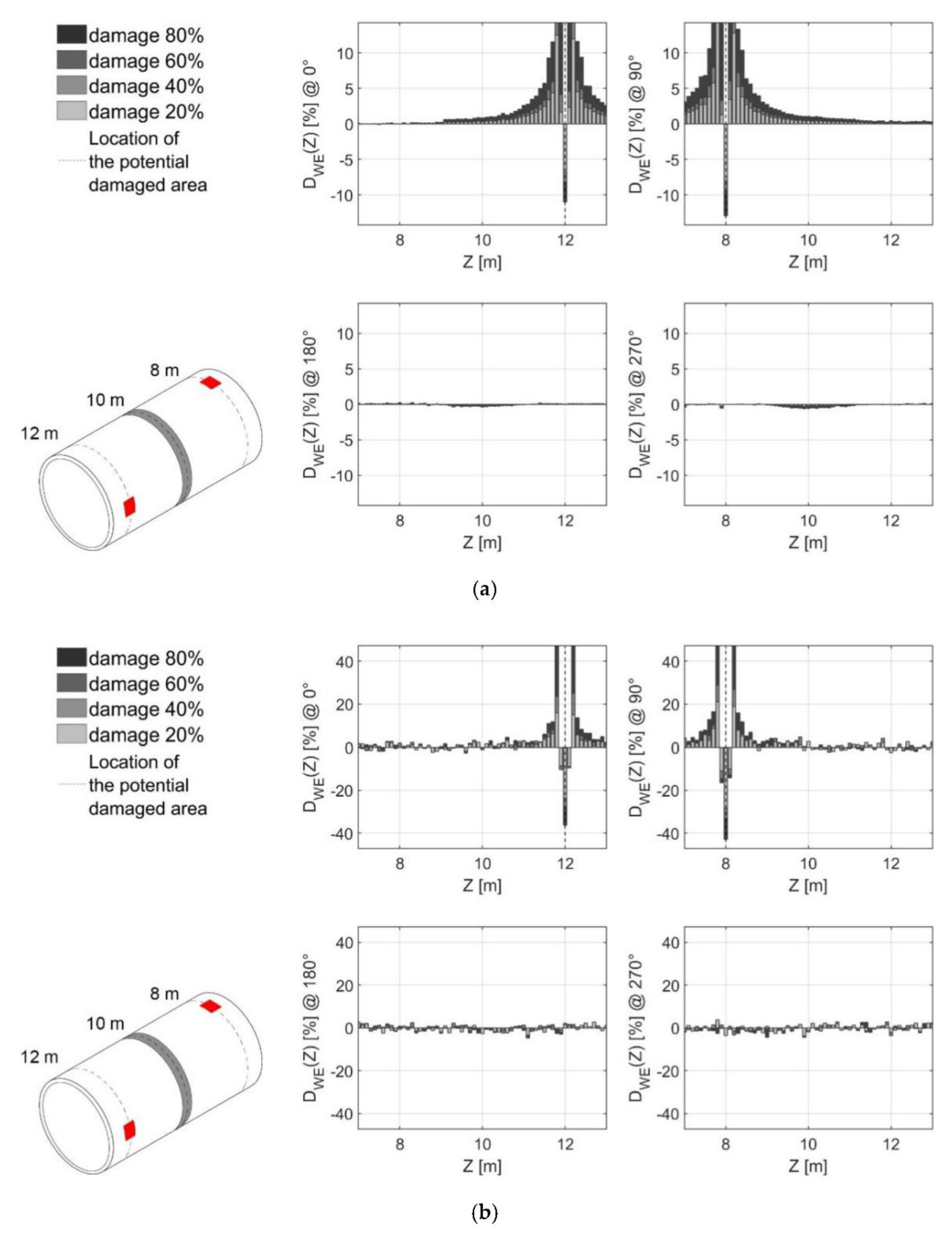
5.1. Multiple Damage Detection and Localisation
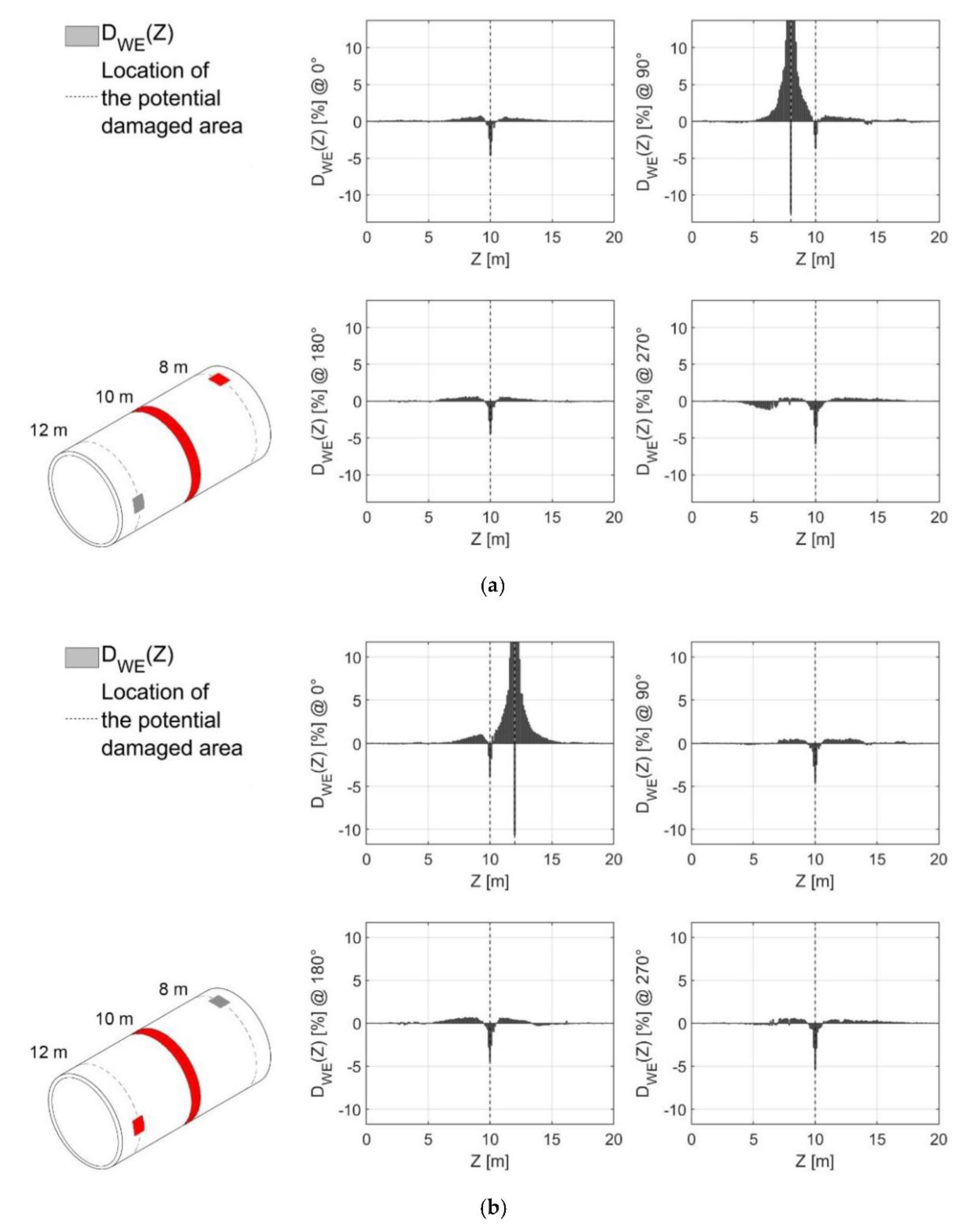
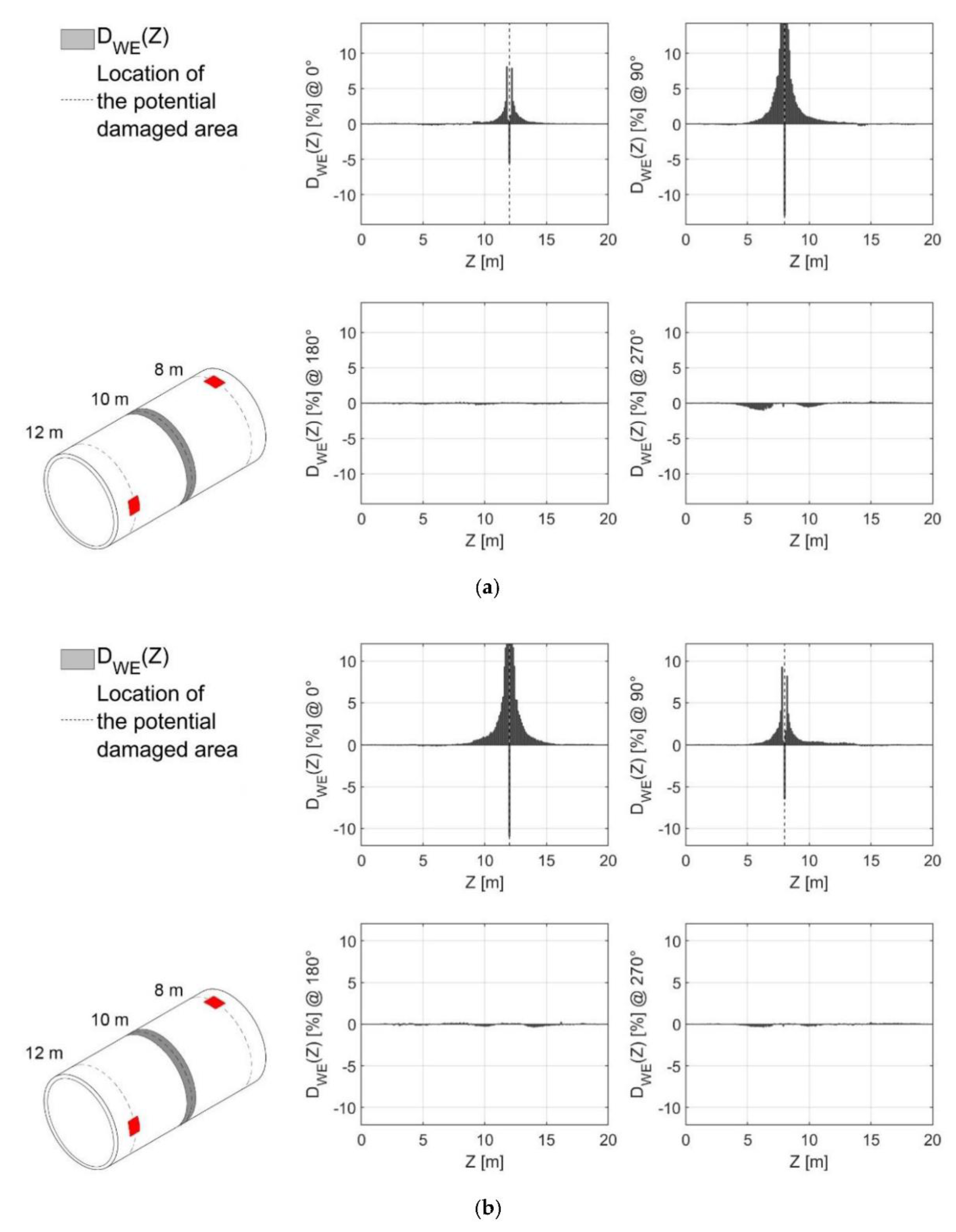
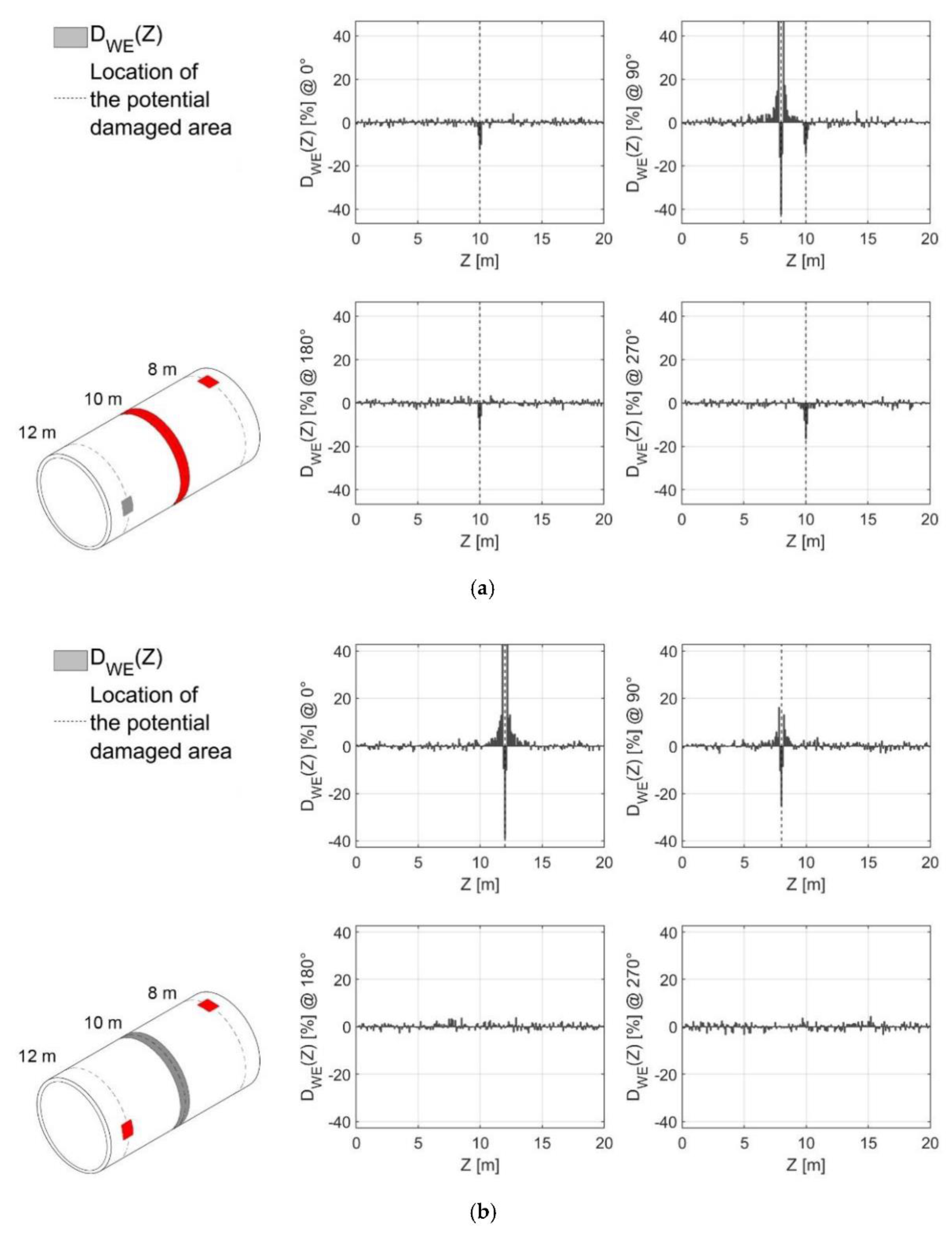
Four damage scenarios are here reported: 80%/20%/0% and its specular 0%/20%/80%, plus 80%/0%/40% and its specular 40%/0%/80%. In the first two cases, one localized and one large-spread damaged area were considered. In the latter pair, the two smaller damaged areas were included, with alternating severity, while the ring-like damage was deactivated. These two sets are reported, respectively, in
Figure 5 and
Figure 6. Both figures report the noise-free results for the optic fibers deployed at
and
in the upper row (left and right plots, respectively) and for
and
in the lower row (in the same order).
As expected, the insertion of the damage caused a localized decrease of the Wiener entropy. This confirms the findings of previous studies [
10,
11,
17].
As can be seen, the variation in the measured WE depended both on the z- and the -coordinate. This allowed us to locate the damaged portion(s) in cylindrical coordinates.
In both
Figure 5a,b, the ring-like damage #2 is visible in all four fibers (
θ = 0°, 90°, 180°, and 270°). It is possible to infer from this the existence of one large example of damage and therefore to evaluate its large spatial extension (although, potentially, the same results might be due to four distinct damages located at the same z coordinates; this ambiguity cannot be solved with the spatial resolution applied in this case study, i.e., 0.10 m). On the other hand, the two smaller examples of damage are only detected by their closest sensor (
and
, respectively).
In noise-free conditions, the insertion of perfectly identical damage at different locations returned identical changes in the spatial distribution of the spectral flatness index. This can be easily visualized in the second set of results as well (
Figure 6).
Effects of Artificially Added Noise
Figure 7 reports the results for the damage scenarios with an artificially added 10% noise. The two cases portrayed there represent the two combinations, with 80%/20%/0% and 40%/0%/80%. These can be directly compared with
Figure 5a and
Figure 6b, respectively. One can see that the presence of noise causes the effects of damage to decay more rapidly, moving away from the damage location. In the exact damage location, the inhomogeneity effects are noticeable and even increased significantly in their absolute value. However, this behavior is reached with a contextual absolute value increase of the health state indicator far from the damaged area.
5.2. Multiple Damage Severity Assessment
Figure 8,
Figure 9 and
Figure 10 report the results for increasing damage level in damage #1, #2, and #3 (in the same order), with and without added noise.
It is possible to notice how the entropy-based health state indicator increases monotonically for an increasing damage level, showing thus a correlation between the stiffness reduction and the entropy variation. In contrast, far from the damage, the variability induced by the noise affects the baseline and the damaged structure in a similar fashion. In this way, the two effects cancel each other out, resulting in a near-zero variation. For this reason, the proposed damage indicator is robust to noise in terms of avoided false positives.
The noise affects the sensibility of the indicator, similarly to what is seen in the previous subsection. The same remarks can be applied here: while the damage becomes less detectable from a longer distance, its short-range effects seem to be positively affected by the additional noise, making it more pronounced.
5.3. Single and Multiple Damage Intensity Tracking
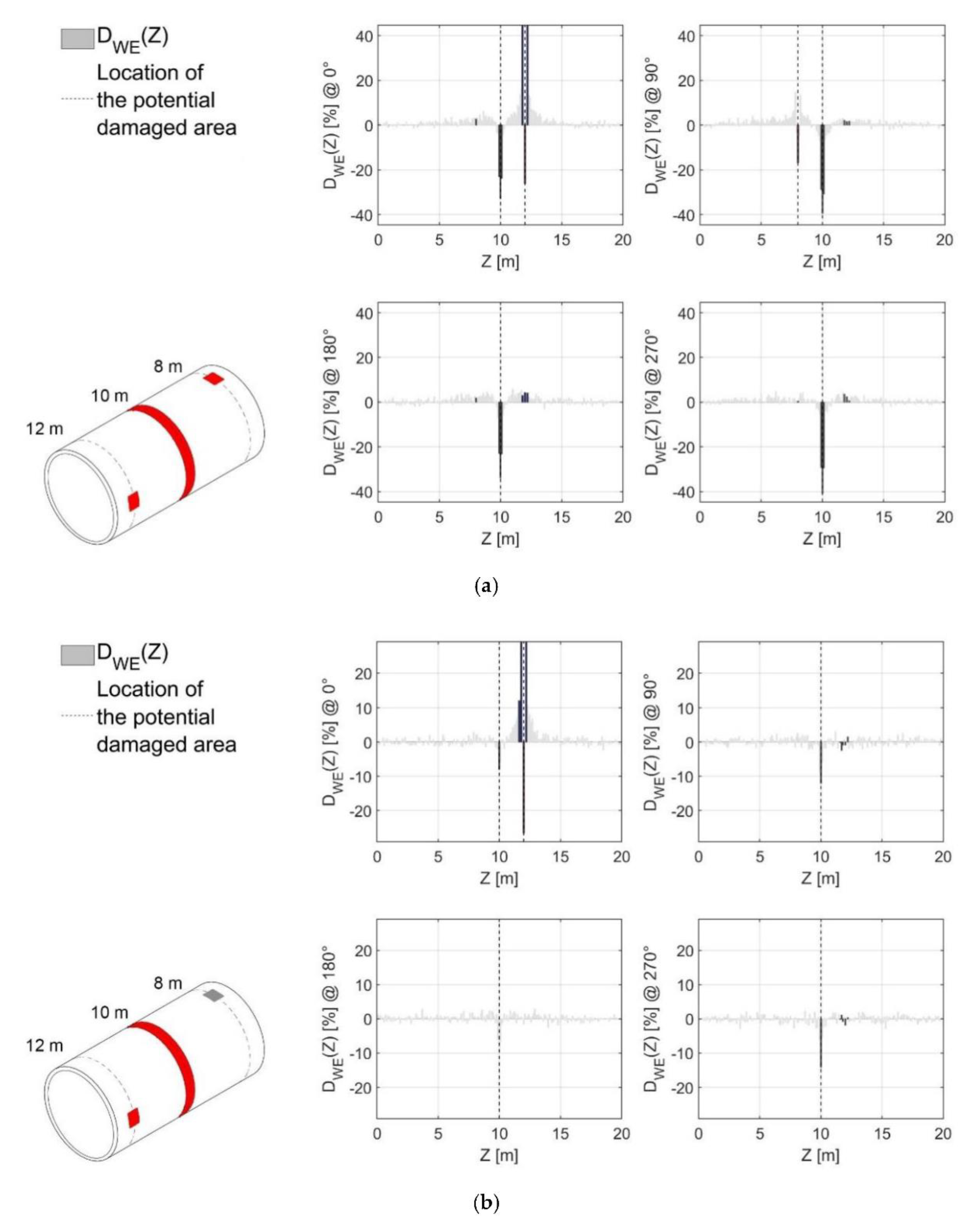
The potentialities of the proposed approach have been tested as well for single and multi-damage tracking. Indeed, buried structures might not always be easily accessible for maintenance and reparation. Furthermore, a certain degree of damage tolerance is always considered at the design stage (see, e.g., [
55]). Thus, it is possible that, due to practical or economic constraints, one or more examples of damage detected are not immediately repaired but rather put under surveillance. These examples of damage are then expected to extend over time, with an increase in their severity. Furthermore, other unrelated damage may occur nearby, compromising the already endangered situation.
Figure 11 reports a damage pattern with 40%/60%/80% stiffness reduction. This can be considered as a scenario where, following the already damaged conditions portrayed in
Figure 6b, a joint failure suddenly happens in the pipe section in-between the two pre-existent damages. By comparing these two cases (with and without artificial noise), one can see that the effects of damage #2 combine with the effects of the previous damages in
θ = 0° and 90°, while also being detectable elsewhere as expected. Adding artificial noise to the measurement does not significantly affect the results.
Similarly,
Figure 12a,b depict a damage increase from 50%/0%/50% to 60%/0%/60% and 80%/0%/80% (for the noise-free and noise = 10% cases, respectively), emulating, e.g., uniform crack growth or corrosion progress at both locations. In this case, it is possible to note that the increase in the absolute value of the health state indicator can be perceived already by moving from 50%/0%/50% to 60%/0%/60% of stiffness reduction. Then, the increase is even more pronounced moving from the damage case 60%/0%/60% to 80%/0%/80%. The results are also quite consistent in the presence of a relatively high level of noise (i.e., 10%).
In conclusion, comparing the different damage steps allows detecting the increasing reduction of WE after each subsequent additional damage. This does not allow precise estimates, yet permits some qualitative assessment of the worsening of the pipeline’s structural integrity at those points already damaged.
5.4. Applications for Unsupervised Learning
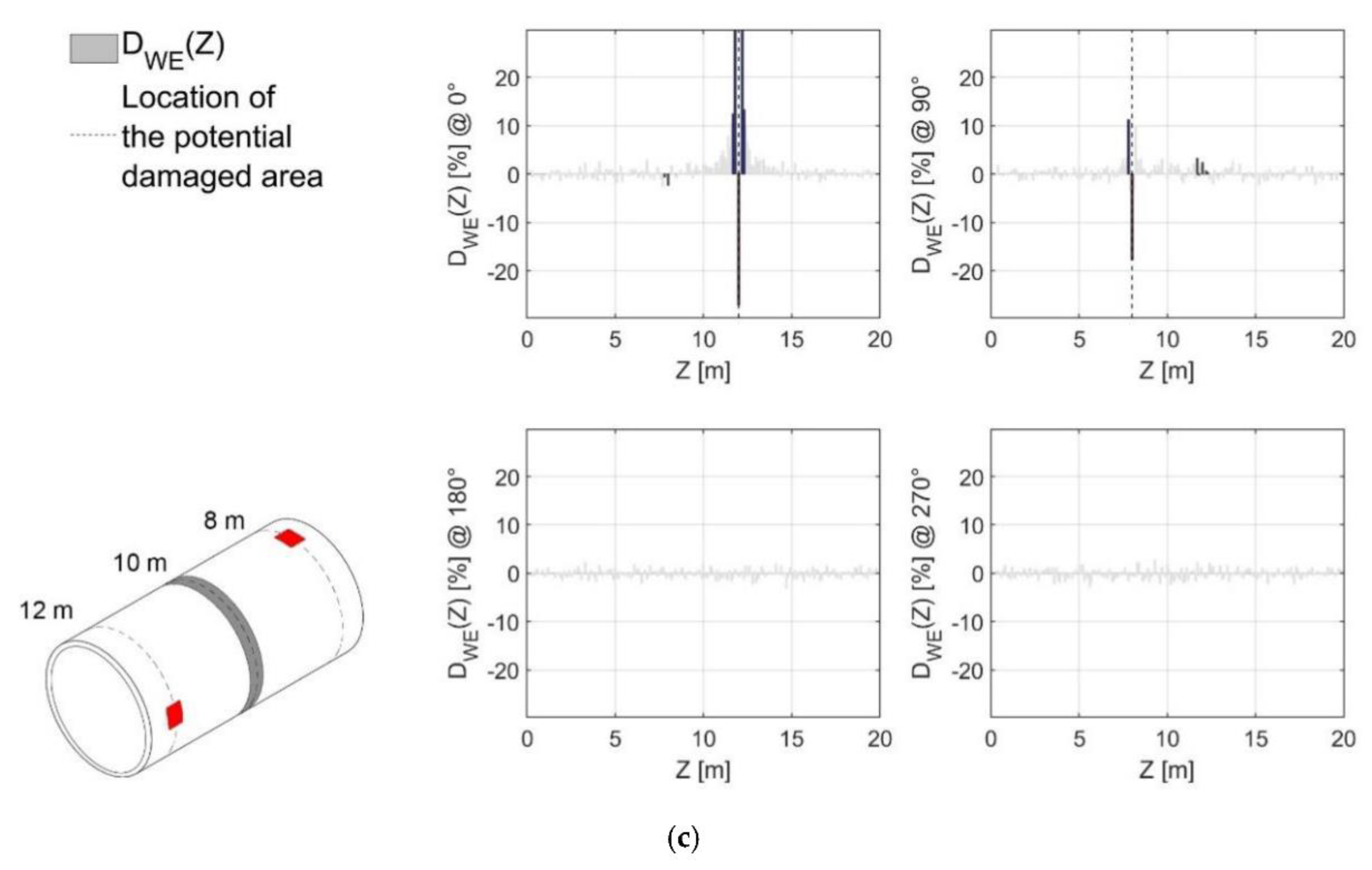
The results presented so far demonstrate how Wiener entropy can define a reliable damage-sensible feature. Its feasibility for machine learning-based SHM can be demonstrated by using it as a training dataset for a pattern recognition technique. Specifically, a simple method for detecting and localizing damage based on outlier detection analysis has been chosen for this aim. The 3-sigma method defines a threshold value for the ‘normality’ model at 3σ, i.e., corresponding to a 99.73% confidence interval if data are Gaussian distributed. This classic approach is commonly used to test newly-proposed DSFs (as done, e.g., in [
56]) due to both its simplicity, its statistically principled bases, but also its well-known limitations. It is known that the 3-sigma rule is an empirical method [
57]; in addition, if data deviate from a Gaussian distribution, the basic assumption of this method is lost. Thus, any valid result obtained by training a damage detection/localization algorithm with the proposed feature can only be improved by applying more recent, sophisticated options. This, however, falls beyond the aim of this paper, that instead takes advantage of the use of non-robust outlier classification methods (i.e., 3-sigma method), which intrinsically define the robustness and the noise rejection capability of the WE as a damage-sensitive feature, estimated starting from random ambient vibrations data.
The results are here statistically described in terms of precision and recall, calculated from the total numbers of false positives and negatives (
fp and
fn) and true positives
tp as follows:
It is possible to note from the results that all of the damage scenarios have relatively high precision and recall. For the precision it is worth underling that the results are quite variable based on the meaning that is given to the class “False positive”, as can be perceived by
Table 3. This is mainly because all of the false positives automatically detected are associated with a point located close to a damaged area. For example, when the damage occurs at
z = 8 m (
), and
z = 12 m (
), the false positives are related to the effect of damage that occurs at
z = 12 m (
), which is perceived by sensors located at
z = 12 m, and
, or vice versa. The same applies to damage at
z = 8 m. This was found not only in the damage scenario 40%/60%/80% but also for all the investigated damage scenarios, as shown in
Figure 13. In fact, in a real SHM scenario, such “false positives” could be a benefit as they should help to strengthen the localization of the damage thanks to considerations on the amplitude of variation of WE. This because all of the “false positives” have a value of the health state indicator
that is very close to zero. If the damage detected by the sensors placed near to the damaged area is not considered as a “false positive”, then the number of false positives is zero (with the 3-sigma outliers detection method), as reported in
Table 3. Regarding the recall, it is possible to conclude that a relatively high value, 90.69%, is obtained by considering all damage scenarios.
5.5. Potential Applications for Supervised Learning
To conclude this investigation, it might be useful to say that, if available, a catalog of expected entropy changes caused by different damage typologies (such as the ones described in
Section 3) could be used for supervised learning, providing a machine learning (ML) system with some damage classification (or even damage prognosis) capabilities. However, these aspects will require further studies.
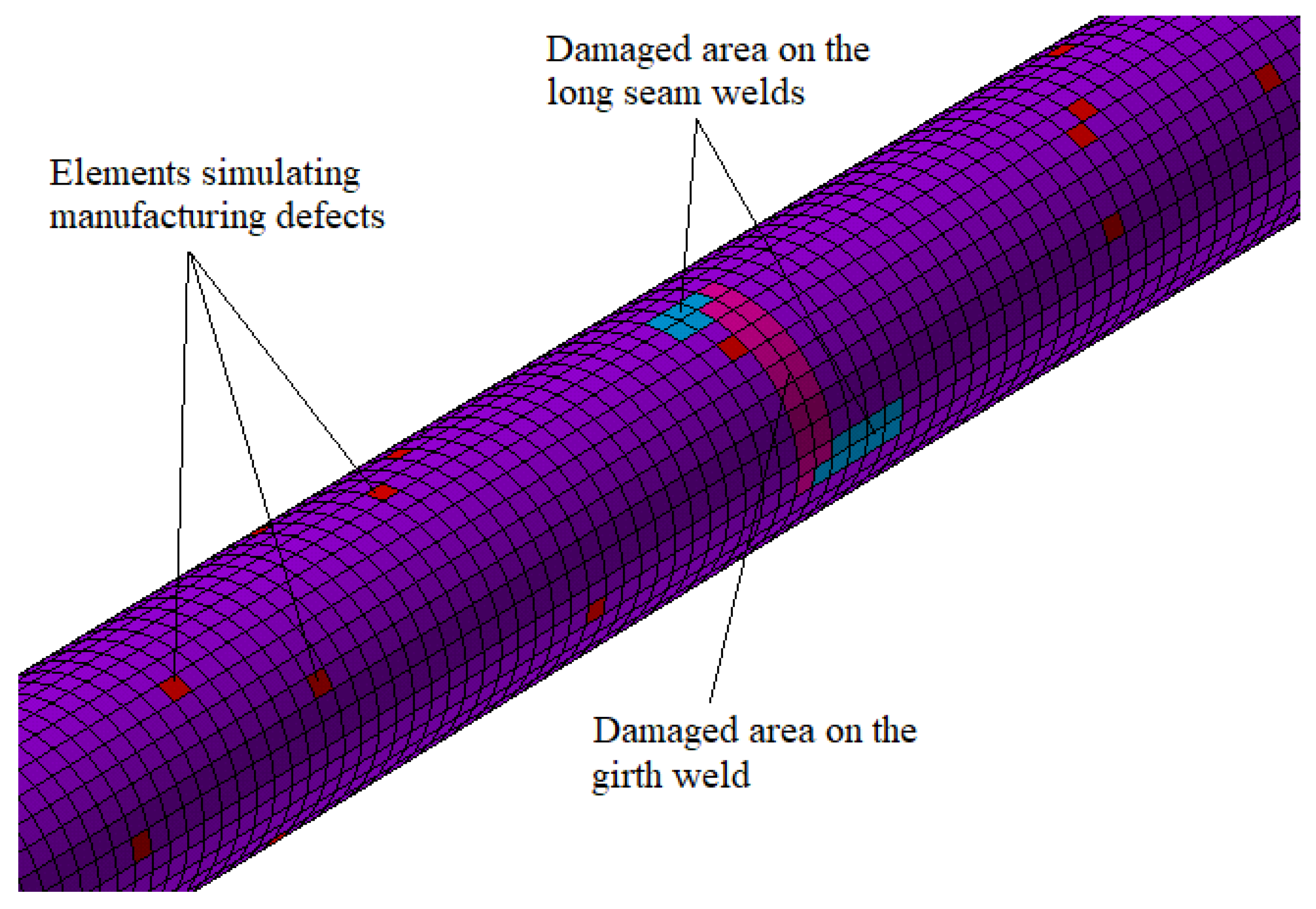
6. Accounting for Uncertainties
To conclude this research, a last set of tests were reserved for a more realistic FE model (shown in
Figure 14).
Specifically, having validated the algorithm under ideal conditions, this further test included more realistic assumptions about the material properties. Since the second FE model shares most of the mechanical and geometrical properties of the first case study, only the major differences will be commented on hereafter.
A random perturbation of the soil parameters over all the springs of the FE model resulted in a random deviation from the nominal value of the first model of about 20% (+-10%). This was intended to emulate the inhomogeneity of the surrounding material soil.
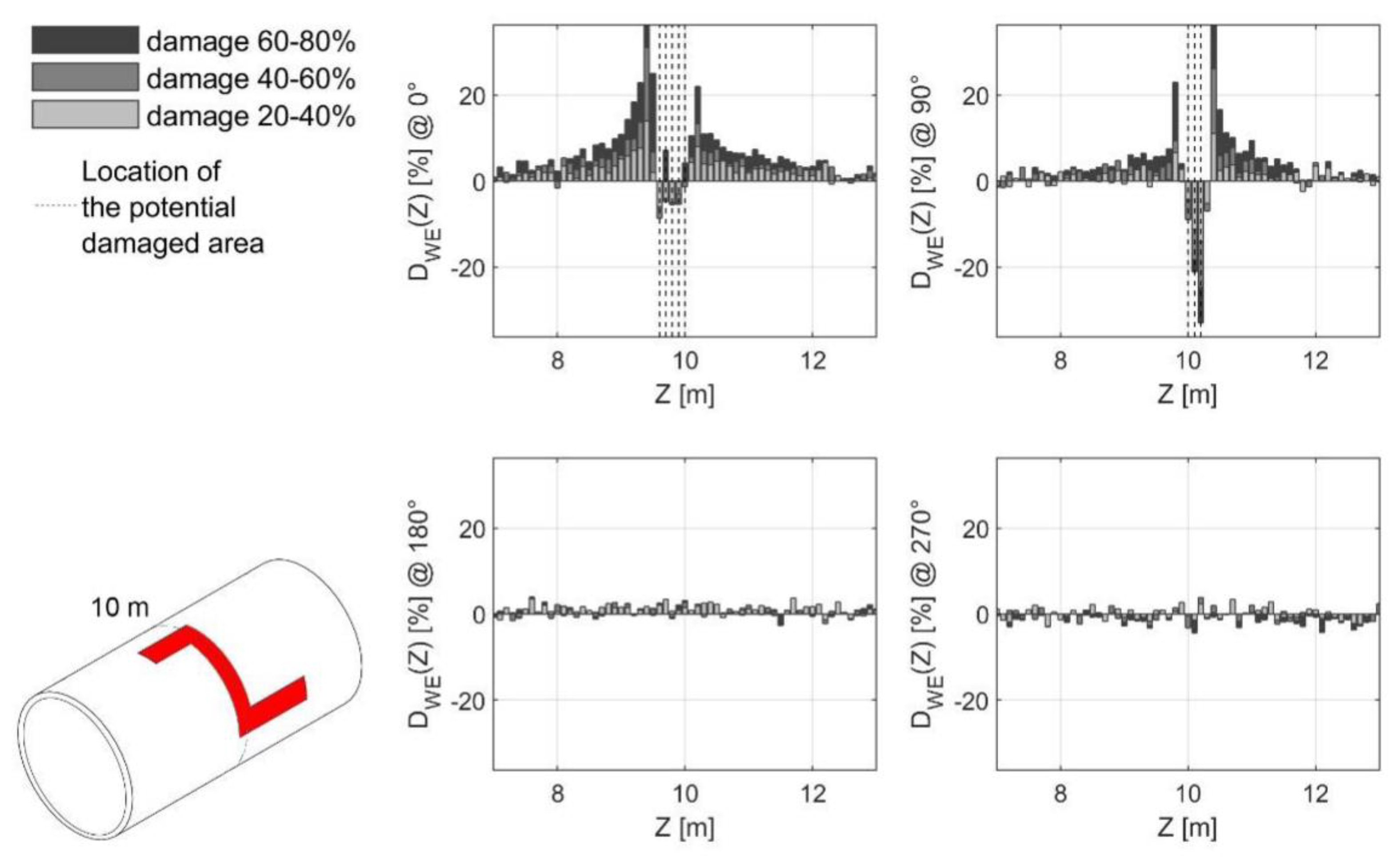
A reduction of 10% of Young’s modulus of 75 randomly selected finite elements of the SP model was assumed to simulate the presence of manufacturing defects. At the same time, a reduction of stiffness of 20%, 40%, and 60% was assumed to simulate damage on the girth weld, located at 10 m (at the center of the analyzed SP) from 0° to 90°; while a reduction of stiffness of 40%, 60%, and 80% was assumed to simulate damage on two long seam welds, located at 0° (from 9.5 to 10 m) and 90° (from 10 to 9.20 m). This was intended to simulate an S-shaped crack on the pipeline similar to the one shown previously in
Figure 1 at the intersection between the girth and two consecutive long seam welds. A constant width of 0.16 m was applied for the damage in the two long seam welds, while a width of 0.20 m was considered for the damage in the girth weld.
To summarize, three steps of increasing damage were introduced, considering the following stiffness reduction on the circumferential tract and the two longitudinal ones (in the same order): 20% and 40%; 40% and 60%; 60% and 80%. As for the previous case study, artificial WGN between 5% and 20% of the standard deviation of the output signals was added to the simulated output responses. For brevity, only results for 5% noise are reported in
Figure 15, as was already done for the first model.
From
Figure 15 it is possible to conclude that also in presence of inhomogeneity of the surrounding soil and manufacturing defects the Wiener entropy of axial strains was able to detect and locate quite well the damage. The same considerations can be performed for other percentages of noise, while an instability was observed in the absence of noise in data, for the damage at 0°. However, as concluded in [
10], this is a known behavior of Wiener entropy, which needs the addition of numerical noise to stabilize the health state indicator estimate.
7. Conclusions
This paper described the use of Wiener entropy for pipeline integrity management and structural health monitoring of buried steel pipes.
In general terms, the undergoing establishment of an entropic framework for SHM strongly supports the main concepts of entropy measurements as an indicator for health state development. A quantifiable decrease in the WE signal entropy in operational conditions can be directly linked to a localized decrease of material stiffness when strain measurements are used as a structural sensing response.
For unchanged boundary conditions, this can be further linked to developing one or more damages in the structure under investigation.
Regarding the specific case study discussed here, the motivations for using the proposed procedure to underground metallic structures have been highlighted. As long as the input spectral flatness is guaranteed by the use of ambient vibrations, the use of a spectral flatness measurement on the system output is entirely logical. This allows for precise assessment for very low amplitude output signals, where traditional techniques struggle or completely fail, thanks to the non-deterministic behavior of the target system. Two FE models were employed and several damage patterns were applied to them.
The WE-based procedure was applied for several SHM tasks, defined accordingly to the classic Rytter’s hierarchy. The main findings can be summarized as follows:
- −
The small extension and severity of some cases highlighted the capabilities of the proposed indicator to detect stiffness reduction at an early stage, thus avoiding the insurgence of latent damages;
- −
The proposed approach can detect and assess multiple damages of different sizes and severities;
- −
The simple health state indicator proved the robustness of the monitoring of WE of strain also in the presence of artificially added measurement noise;
- −
The proposed approach performed well both under ideal (yet unrealistic) conditions and with initial flaws and soil inhomogeneities.
As expected, it was noted that the WE of the simulated output signals (axial strains) locally decreases for local stiffness reductions. It was also noticed that it increases immediately outside the damaged area; this becomes more pronounced as the damage increases. This aspect will be further addressed in future works. Further studies will be needed to better address specific tasks, such as damage classification, which strictly requires pattern recognition techniques in a supervised learning fashion. Nevertheless, this study proved the feasibility of Wiener entropy as a damage-sensitive feature for vibration-based inspection, particularly well-suited for output-only measurements of underground structures.
Author Contributions
Conceptualization, R.C., M.C., G.M. and E.L.; methodology, R.C., M.C., G.M. and E.L.; software, G.M., M.C. and E.L.; validation, G.M., M.C. and E.L.; resources, R.C.; data curation, G.M., M.C. and E.L.; writing—original draft preparation, M.C., G.M. and E.L.; writing—review and editing, R.C., G.M. and E.L.; visualization, M.C., G.M. and E.L.; supervision, R.C. and C.S.; project administration, R.C. and C.S. All authors have read and agreed to the published version of the manuscript.
Funding
This research received no external funding.
Data Availability Statement
The data that support the findings of this study are available from the authors upon reasonable request.
Conflicts of Interest
The authors declare no conflict of interest.
References
- Sethna, J.P. Statistical Mechanics: Entropy, Order Parameters, and Complexity; Oxford University Press: Oxford, UK, 2006. [Google Scholar]
- Farrar, C.; Worden, K.; Park, G. Complexity: A New Axiom for Structural Health Monitoring? 2010. Available online: https://www.semanticscholar.org/paper/Complexity%3A-A-New-Axiom-for-Structural-Health-Farrar-Park/4209f3dd65f98f741fb73241adade9f16df3a8b4 (accessed on 14 June 2021).
- West, B.M.; Locke, W.R.; Andrews, T.C.; Scheinker, A.; Farrar, C.R. Applying Concepts of Complexity to Structural Health Monitoring. In Structural Health Monitoring, Photogrammetry & DIC; Springer: Cham, Switzerland, 2019; Volume 6, pp. 205–215. [Google Scholar] [CrossRef]
- Worden, K.; Farrar, C.R.; Manson, G.; Park, G. The fundamental axioms of structural health monitoring. Proc. R. Soc. A Math. Phys. Eng. Sci. 2007, 463, 1639–1664. [Google Scholar] [CrossRef]
- Hill, M.O. Diversity and Evenness: A Unifying Notation and Its Consequences. Ecology 1973, 54, 427–432. [Google Scholar] [CrossRef] [Green Version]
- Das, A.K.; Leung, C.K.Y. Power Spectral Entropy (PSE) as a Qualitative Damage Indicator. In Proceedings of the 9th European workshop on structural health monitoring (EWSHM-2018), Manchester, UK, 10–13 July 2018. [Google Scholar]
- Lin, T.-K.; Chien, Y.-H. Performance Evaluation of an Entropy-Based Structural Health Monitoring System Utilizing Composite Multiscale Cross-Sample Entropy. Entropy 2019, 21, 41. [Google Scholar] [CrossRef] [Green Version]
- Amiri, M.; Modarres, M. An Entropy-Based Damage Characterization. Entropy 2014, 16, 6434–6463. [Google Scholar] [CrossRef] [Green Version]
- Donajkowski, H.; Leyasi, S.; Mellos, G.; Farrar, C.R.; Scheinker, A.; Pei, J.-S.; Lieven, N.A.J. Comparison of Complexity Measures for Structural Health Monitoring; Springer: Cham, Switzerland, 2020; pp. 27–39. [Google Scholar]
- Ceravolo, R.; Lenticchia, E.; Miraglia, G. Spectral entropy of acceleration data for damage detection in masonry buildings affected by seismic sequences. Constr. Build. Mater. 2019, 210, 525–539. [Google Scholar] [CrossRef]
- Ceravolo, R.; Lenticchia, E.; Miraglia, G. Use of Spectral Entropy for Damage Detection in Masonry Buildings in the Presence of Mild Seismicity. Proceedings 2018, 2, 432. [Google Scholar] [CrossRef] [Green Version]
- Gelman, L.; Kırlangıç, A.S. Novel vibration structural health monitoring technology for deep foundation piles by non-stationary higher order frequency response function. Struct. Control. Health Monit. 2020, 27. [Google Scholar] [CrossRef]
- Civera, M.; Zanotti Fragonara, L.; Surace, C. A novel approach to damage localisation based on bispectral analysis and neural network. Smart Struct. Syst. 2017, 20, 669–682. [Google Scholar]
- Ubertini, F.; Comanducci, G.; Cavalagli, N. Vibration-based structural health monitoring of a historic bell-tower using output-only measurements and multivariate statistical analysis. Struct. Health Monit. 2016, 15, 438–457. [Google Scholar] [CrossRef]
- Rytter, A. Vibrational Based Inspection of Civil Engineering Structures. Ph.D. Thesis, Aalborg University, Aalborg, Denmark, 1993. [Google Scholar]
- Worden, K.; Dulieu-Barton, J.M. An Overview of Intelligent Fault Detection in Systems and Structures. Struct. Health Monit. 2004, 3, 85–98. [Google Scholar] [CrossRef]
- Civera, M.; Ceravolo, R.; Lenticchia, E.; Miraglia, G.; Surace, C. Damage Detection and Localisation in Buried Pipelines using Entropy in Information Theory. In Proceedings of the 1st International Electronic Conference on Applied Sciences, Online, 10–30 November 2020; pp. 30–36. [Google Scholar] [CrossRef]
- Martucci, D.; Civera, M.; Surace, C. The Extreme Function Theory for Damage Detection: An Application to Civil and Aerospace Structures. Appl. Sci. 2021, 11, 1716. [Google Scholar] [CrossRef]
- Barron, A.R. Entropy and the Central Limit Theorem. Ann. Probab. 1986, 14, 336–342. [Google Scholar] [CrossRef]
- Farrar, C.R.; Doebling, S.W.; Nix, D.A. Vibration–based structural damage identification. Philos. Trans. R. Soc. A Math. Phys. Eng. Sci. 2001, 359, 131–149. [Google Scholar] [CrossRef]
- Oh, C.K.; Sohn, H. Damage diagnosis under environmental and operational variations using unsupervised support vector machine. J. Sound Vib. 2009, 325, 224–239. [Google Scholar] [CrossRef]
- Cross, E.; Manson, G.; Worden, K.; Pierce, S. Features for damage detection with insensitivity to environmental and operational variations. Proc. R. Soc. A Math. Phys. Eng. Sci. 2012, 468, 4098–4122. [Google Scholar] [CrossRef]
- Pecorelli, M.L.; Ceravolo, R.; Epicoco, R. An Automatic Modal Identification Procedure for the Permanent Dynamic Monitoring of the Sanctuary of Vicoforte. Int. J. Arch. Heritage 2018, 14, 630–644. [Google Scholar] [CrossRef]
- Transportation Research Board. Introduction. In Transmission Pipelines and Land Use: A Risk-Informed Approach—Special Report 281; Transportation Research Board: Washington, DC, USA, 2004; Chapter 1. [Google Scholar]
- Chmelko, V.; Garan, M.; Šulko, M.; Gašparík, M. Health and Structural Integrity of Monitoring Systems: The Case Study of Pressurized Pipelines. Appl. Sci. 2020, 10, 6023. [Google Scholar] [CrossRef]
- A Papadakis, G. Assessment of requirements on safety management systems in EU regulations for the control of major hazard pipelines. J. Hazard. Mater. 2000, 78, 63–89. [Google Scholar] [CrossRef]
- Transportation Research Board. Approach for Risk-Informed Guidance in Land Use Planning. In Transmission Pipelines and Land Use: A Risk-Informed Approach—Special Report 281; Transportation Research Board: Washington, DC, USA, 2004; Chapter 3. [Google Scholar]
- Whidden, W.R. Buried Flexible Steel Pipe: Design and Structural Analysis; American Society of Civil Engineers: Reston, VA, USA, 2009. [Google Scholar]
- Rizzo, P. Water and Wastewater Pipe Nondestructive Evaluation and Health Monitoring: A Review. Adv. Civ. Eng. 2010, 2010, 1–13. [Google Scholar] [CrossRef] [Green Version]
- Civera, M.; Boscato, G.; Fragonara, L.Z. Treed gaussian process for manufacturing imperfection identification of pultruded GFRP thin-walled profile. Compos. Struct. 2020, 254, 112882. [Google Scholar] [CrossRef]
- Piccinelli, R.; Krausmann, E. Analysis of Natech Risk for Pipelines: A Review; Publications Office of the European Union Luxembourg: Luxembourg, 2013. [Google Scholar]
- Cosham, A.; Hopkins, P. The effect of dents in pipelines—guidance in the pipeline defect assessment manual. Int. J. Press. Vessel. Pip. 2004, 81, 127–139. [Google Scholar] [CrossRef]
- Kishawy, H.A.; Gabbar, H.A. Review of pipeline integrity management practices. Int. J. Press. Vessel. Pip. 2010, 87, 373–380. [Google Scholar] [CrossRef]
- Lu, H.; Iseley, T.; Behbahani, S.; Fu, L. Leakage detection techniques for oil and gas pipelines: State-of-the-art. Tunn. Undergr. Space Technol. 2020, 98, 103249. [Google Scholar] [CrossRef]
- Datta, S.; Sarkar, S. A review on different pipeline fault detection methods. J. Loss Prev. Process. Ind. 2016, 41, 97–106. [Google Scholar] [CrossRef]
- Alobaidi, W.M.; Alkuam, E.A.; Al-Rizzo, H.M.; Sandgren, E. Applications of Ultrasonic Techniques in Oil and Gas Pipeline Industries: A Review. Am. J. Oper. Res. 2015, 5, 274–287. [Google Scholar] [CrossRef] [Green Version]
- Giunta, G.; Budano, S.; Lucci, A.; Prandi, L. Pipeline Health Integrity Monitoring (PHIM) Based on Acoustic Emission Technique. In Proceedings of the Pressure Vessels and Piping Conference. American Society of Mechanical Engineers, Toronto, QC, Canada, 15–19 July 2012; Volume 5, pp. 277–283. [Google Scholar] [CrossRef]
- Quarini, J.; Shire, S. A Review of Fluid-Driven Pipeline Pigs and their Applications. Proc. Inst. Mech. Eng. Part E J. Process. Mech. Eng. 2007, 221, 1–10. [Google Scholar] [CrossRef]
- Liu, Z.; Kleiner, Y. State-of-the-Art Review of Technologies for Pipe Structural Health Monitoring. IEEE Sens. J. 2012, 12, 1987–1992. [Google Scholar] [CrossRef]
- Pipeline Safety Trust. Pipeline Basics & Specifics about Natural Gas Pipelines. Pipeline Safety Trust. Available online: https://www.pstrust.org/wp-content/uploads/2015/09/2015-PST-Briefing-Paper-02-NatGasBasics.pdf (accessed on 14 June 2021).
- Swamee, P.K.; Sharma, A.K. Design of Water Supply Pipe Networks; Wiley: Hoboken, NJ, USA, 2008. [Google Scholar]
- European Commission. EN 1993-1-1:2005 & AC 2:2009—Sections 3.2.1 and 3.2.6; European Commission: Brussels, Belgium, 2005. [Google Scholar]
- Norsok Standardisation Work Group. Material Data Sheets for Piping—Norsok Standard Common Requirements; Norsok Standardisation Work Group: Lysaker, Norway, 1994. [Google Scholar]
- Adhikari, S.; Bhattacharya, S. Vibrations of wind-turbines considering soil-structure interaction. Wind. Struct. Int. J. 2011, 14, 85–112. [Google Scholar] [CrossRef] [Green Version]
- Acerra, C.; Havenith, H.B.; Zacharopoulos, S. Guidelines for the Implementation of the H/V Spectral Ratio Technique on Ambient Vibrations Measurements, Processing and Interpretation; European Commission: Brussels, Belgium, 2004. [Google Scholar]
- Bard, P.-Y. Microtremor measurements: A tool for site effect estimation. Eff. Surf. Geol. Seism. Motion 1999, 3, 1251–1279. [Google Scholar]
- Gutenberg, B. Microseisms. Adv. Geophys. 1958, 5, 53–92. [Google Scholar] [CrossRef]
- Asten, M.; Henstridge, J.D. Array estimators and the use of microseisms for reconnaissance of sedimentary basins. Geophysics 1984, 49, 1828–1837. [Google Scholar] [CrossRef]
- Albarello, D.; Lunedei, E. Structure of an ambient vibration wavefield in the frequency range of engineering interest ([0.5, 20] Hz): Insights from numerical modelling. Near Surf. Geophys. 2011, 9, 543–559. [Google Scholar] [CrossRef]
- Bonnefoy-Claudet, S.; Cotton, F.; Bard, P.-Y. The nature of noise wavefield and its applications for site effects studies: A literature review. Earth Sci. Rev. 2006, 79, 205–227. [Google Scholar] [CrossRef]
- Glisic, B.; Yao, Y. Fiber optic method for health assessment of pipelines subjected to earthquake-induced ground movement. Struct. Health Monit. 2012, 11, 696–711. [Google Scholar] [CrossRef]
- Othonos, A. Fiber Bragg gratings. Rev. Sci. Instrum. 1997, 68, 4309–4341. [Google Scholar] [CrossRef]
- Papadopoulos, C.; Dimarogonas, A. Coupled longitudinal and bending vibrations of a rotating shaft with an open crack. J. Sound Vib. 1987, 117, 81–93. [Google Scholar] [CrossRef]
- Civera, M.; Pecorelli, M.L.; Ceravolo, R.; Surace, C.; Fragonara, L.Z. A multi-objective genetic algorithm strategy for robust optimal sensor placement. Comput. Civ. Infrastruct. Eng. 2021. [Google Scholar] [CrossRef]
- Rosenfeld, M.J.; Pepper, J.W.; Leewis, K. Basis of the New Criteria in ASME B31.8 for Prioritization and Repair of Mechanical Damage. In Proceedings of the 4th International Pipeline Conference, Parts A and B, Calgary, AB, Canada, 30 September–3 October 2002; ASME International: New York, NY, USA, 2002; pp. 647–658. [Google Scholar]
- Civera, M.; Surace, C. A Comparative Analysis of Signal Decomposition Techniques for Structural Health Monitoring on an Experimental Benchmark. Sensors 2021, 21, 1825. [Google Scholar] [CrossRef]
- Lehmann, R. 3σ-Rule for Outlier Detection from the Viewpoint of Geodetic Adjustment. J. Surv. Eng. 2013, 139, 157–165. [Google Scholar] [CrossRef] [Green Version]
Figure 2.
The multi-modeling approach: (a) plain strain FE model of soil; (b) plain strain FE model of soil and SP; (c) plain strain FE model of SP and springs; and (d) 3D FE model of SP and springs. The global reference system is well depicted in (c).
Figure 2.
The multi-modeling approach: (a) plain strain FE model of soil; (b) plain strain FE model of soil and SP; (c) plain strain FE model of SP and springs; and (d) 3D FE model of SP and springs. The global reference system is well depicted in (c).
Figure 3.
The layout of the simulated optic fibers.
Figure 3.
The layout of the simulated optic fibers.
Figure 4.
The location of the three damaged areas.
Figure 4.
The location of the three damaged areas.
Figure 5.
The first set of multi-damaged scenarios: (a) 80%/20%/0%; (b) 0%/20%/80%. Noise-free measurements.
Figure 5.
The first set of multi-damaged scenarios: (a) 80%/20%/0%; (b) 0%/20%/80%. Noise-free measurements.
Figure 6.
The second set of multi-damaged scenarios: (a) 80%/0%/40%; (b) 40%/0%/80%. Noise-free measurements.
Figure 6.
The second set of multi-damaged scenarios: (a) 80%/0%/40%; (b) 40%/0%/80%. Noise-free measurements.
Figure 7.
Noisy measurements (10% of noise): (a) 80%/20%/0%; (b) 40%/0%/80%.
Figure 7.
Noisy measurements (10% of noise): (a) 80%/20%/0%; (b) 40%/0%/80%.
Figure 8.
Increasing stiffness reduction (20%, 40%, 60%, and 80%) for damage #1. (a) noise-free; (b) noise = 10%. Graphs are limited between 7 m and 13 m to show the increase of the intensity of damage for increasing stiffness reduction.
Figure 8.
Increasing stiffness reduction (20%, 40%, 60%, and 80%) for damage #1. (a) noise-free; (b) noise = 10%. Graphs are limited between 7 m and 13 m to show the increase of the intensity of damage for increasing stiffness reduction.
Figure 9.
Increasing stiffness reduction (20%, 40%, 60%, and 80%) for damage #2. (a) noise-free; (b) noise = 10%. Graphs are limited between 7 m and 13 m to show the increase of the intensity of damage for increasing stiffness reduction.
Figure 9.
Increasing stiffness reduction (20%, 40%, 60%, and 80%) for damage #2. (a) noise-free; (b) noise = 10%. Graphs are limited between 7 m and 13 m to show the increase of the intensity of damage for increasing stiffness reduction.
Figure 10.
Increasing stiffness reduction (20%, 40%, 60%, and 80%) for damage #3. (a) noise-free; (b) noise = 10%. Graphs are limited between 7 m and 13 m to show the increase of the intensity of damage for increasing stiffness reduction.
Figure 10.
Increasing stiffness reduction (20%, 40%, 60%, and 80%) for damage #3. (a) noise-free; (b) noise = 10%. Graphs are limited between 7 m and 13 m to show the increase of the intensity of damage for increasing stiffness reduction.
Figure 11.
40%/60%/80% damage scenario. (
a) noise-free (to be compared with
Figure 6b); (
b) noise = 10% (to be compared with
Figure 7b).
Figure 11.
40%/60%/80% damage scenario. (
a) noise-free (to be compared with
Figure 6b); (
b) noise = 10% (to be compared with
Figure 7b).
Figure 12.
Increasing stiffness reduction (50%, 60%, and 80%) for damage in #1 and #3: (a) Noise-free measurements; (b) noise = 10%. Graphs are limited between 7 m and 13 m to show the increase of the intensity of damage for increasing stiffness reduction.
Figure 12.
Increasing stiffness reduction (50%, 60%, and 80%) for damage in #1 and #3: (a) Noise-free measurements; (b) noise = 10%. Graphs are limited between 7 m and 13 m to show the increase of the intensity of damage for increasing stiffness reduction.
Figure 13.
Automatic detection and localization of the severity of damage (noise = 5%). The highlighted bars (in red for negative values, blue for positives ones) are related to points that fall outside 3 times the standard deviation of data (i.e., 3-sigma method): (a) damage scenario 40%/60%/80%; (b) damage scenario 0%/20%/80%; (c) damage scenario 40%/0%/80%.
Figure 14.
The second FE model with damage locations, inhomogeneity of the soil material, and manufacturing defects.
Figure 14.
The second FE model with damage locations, inhomogeneity of the soil material, and manufacturing defects.
Figure 15.
Increasing stiffness reduction (20–40%, 40–60%, and 60–80%) for damage in the girth weld and the long seam welds, respectively. Graphs are limited between 7 m and 13 m to show the increase of the intensity of damage for increasing stiffness reduction.
Figure 15.
Increasing stiffness reduction (20–40%, 40–60%, and 60–80%) for damage in the girth weld and the long seam welds, respectively. Graphs are limited between 7 m and 13 m to show the increase of the intensity of damage for increasing stiffness reduction.
Table 1.
Mechanical properties of the FE models.
Table 1.
Mechanical properties of the FE models.
| Carbon Steel Type 235 (EN 1993-1-1 [42]) |
|---|
| Density | * | |
| Young’s modulus | | |
| Poisson’s ratio | | |
Table 2.
The location and extension of the damaged areas.
Table 2.
The location and extension of the damaged areas.
| Damage ID # | zc [m] | θc [°] | size (z × θ) [m] × [°] |
|---|
| Damage #1 | 8 | 90° | 0.20 × 20° |
| Damage #2 | 10 | 0 ÷ 360° (whole circumference) | 0.20 × 360° |
| Damage #3 | 12 | 0° | 0.20 × 20° |
Table 3.
Results of the automatic detection and localization of the severity of damage (noise = 5%).
Table 3.
Results of the automatic detection and localization of the severity of damage (noise = 5%).
| Damage Scenario (on the Right) | 40%/60%/80% | 0%/20%/80% | 40%/0%/80% | Total |
|---|
| Ideal number of true positive | 600 | 500 | 200 | 1300 |
| True positive | 577 | 402 | 200 | 1179 |
| False positive * | 20/0 | 163/0 | 132/0 | 315/0 |
| False negative | 23 | 98 | 0 | 121 |
| Precision * [%] | 96.65/100 | 71.15/100 | 60.24/100 | 78.92/100 |
| Recall [%] | 96.17 | 80.40 | 100 | 90.69 |
| Publisher’s Note: MDPI stays neutral with regard to jurisdictional claims in published maps and institutional affiliations. |
© 2021 by the authors. Licensee MDPI, Basel, Switzerland. This article is an open access article distributed under the terms and conditions of the Creative Commons Attribution (CC BY) license (https://creativecommons.org/licenses/by/4.0/).


 ,
, 


