Article

Abrupt Change Detection Method Based on Features of Lorenz Trajectories

1
School of Mathematics, Computer Science Institute, Northwest Minzu University, Lanzhou 730030, China
2
Institute of Applied Mathematics and Astronomical Calendar, Northwest Minzu University, Lanzhou 730030, China
3
College of Atmospheric Sciences, Chengdu University of Information Technology, Chengdu 610225, China
4
College of Science, Inner Mongolia University of Technology, Hohhot 010051, China
5
Laboratory for Climate Studies, China Meteorological Administration, Beijing 100081, China
6
School of Physical Science and Technology, Yangzhou University, Yangzhou 225009, China
7
Southern Marine Science and Engineering Guangdong Laboratory, Sun Yat-sen University, Zhuhai 510275, China
*
Author to whom correspondence should be addressed.
Atmosphere 2021, 12(6), 781; https://doi.org/10.3390/atmos12060781
Submission received: 28 April 2021 / Revised: 11 June 2021 / Accepted: 14 June 2021 / Published: 17 June 2021

Abstract

:
This paper presents a definition of bifurcation-type abrupt changes based on the bifurcation features of Lorenz trajectories. These abrupt changes are the result of the transition behavior of dynamical system trajectories among different equilibrium regions. We demonstrate that these bifurcation-type jumps can better reflect the nature of abrupt change. In analyzing the features of Lorenz equation trajectories, a dynamical method for detecting bifurcation-type abrupt changes is presented. A numerical solution of the Lorenz equation is adopted, using a curve integral or vector product to construct a time series of positive and negative values. Changes in the sign of this time series accurately determine whether the trajectory is in the right or left equilibrium region, and the points at which the time series is equal to zero are the times at which the trajectory jumps between different equilibrium regions, that is, the occurrence times of bifurcation-type abrupt changes. This method is completely dependent on the dynamical characteristics of the system. A theoretical approach for detecting abrupt climate changes based on the dynamical characteristics of the atmospheric model is described. Compared with the original method of identifying abrupt climate changes, this method has dynamic significance and can detect abrupt changes in multi-dimensional time series. Although this method can be applied theoretically, applications to real atmospheric data first require the data to be smoothed.

1. Introduction

Abrupt changes are common phenomena in nature, and in human and social activities. Such phenomena have been studied in atmospheric science [1], oceanography [2], geology [3], geography [4], botany [5], zoology [6], medical science [7], economics [8], and sociology [9]. The popular description of an abrupt change is the process of jumping from one state to some other state, leading to the transition of the system of interest from one equilibrium state to another. In this transition process, some properties of the system will change significantly, which may have some unpredictable consequences. This is the main focus of research on abrupt changes.
Catastrophe theory uses mathematical models to explain sudden change behavior in the process of system evolution. The mathematical model may be discrete or continuous, and the results may be exact analytical solutions or numerical approximations. The establishment of catastrophe theory can be traced back to 1972 and the systematic research conducted by the French mathematician Thom [10]. Subsequently, the British mathematician Zeeman developed and improved catastrophe theory [11].
Catastrophe theory is related to the stability of the solution of a differential equation. In 1953, Hadamard solved the Cauchy problem of Laplace’s equation, showing that the differential equation is sensitive to the initial value, which means that the solution is unstable, and constructing a famous counter example [12]. The construction of the Lorenz equation in 1963, in which each term has a clear physical meaning, showed that instabilities are not simply an abstract mathematical concept, such as in Hadamard’s counter example. There are also unstable systems in nature, characterized perhaps by the uncertainty of trajectory motion [13], where the origin of this motion uncertainty lies in the trajectory jumping among different equilibrium points. Catastrophe theory has been applied in various disciplines, such as gene mutations in biology [5,6], the adjustment of industrial structures in the field of economics [8], and the study of abrupt climate change in atmospheric science [14]. In all of these fields, catastrophe theory has been used to predict the changing behavior of complex and disordered systems.
In 1992, Fu et al. proposed a universal definition of abrupt climatic change: “the abrupt change is the jumpy transformation phenomenon from one steady state (the stable and sustainable change trend) to another steady state (the stable and sustainable change trend), the performance is a sharp change from one statistical feature to another statistical feature in space and time” [14]. There has been considerable research on abrupt climate change. For instance, Chu discussed the sudden onset of the East Asian monsoon [15,16], Tu et al. derived approximate times for the advance and retreat of the summer monsoon in China [15,17], and in the analysis of the atmospheric circulation over Asia in 1956, Tao et al. identified a jump change during the transitional period from spring to summer [15,18]. On the basis of surface temperature and precipitation data for China from 1961–2006, the variations and abrupt changes in these variables on the Qinghai Tibet Plateau and six other regions of China were detected and compared by Ding et al. [19]. Krishnamurti discussed the characteristics of the Indian monsoon onset using observational station data [20], while Shinoda et al. analyzed the characteristics of seasonal abrupt changes in the global precipitation distribution in 1979 [21]. All of the above studies are based on observational data, which shows that abrupt changes are a common phenomenon in atmospheric motion. The definition of abrupt climatic change proposed by Fu et al. is founded on statistical features [14], but it is important to clarify the meaning of abrupt climatic change from the viewpoint of the dynamic features of the atmospheric system.
On the basis of mathematical physics and atmospheric observation data, Feng et al. have studied various methods of detecting abrupt climate changes. In particular, heuristic segmentation, permutation entropy, and power-law exponent methods have been proposed for detecting and analyzing abrupt changes in climate, allowing the underlying mechanisms to be identified [22,23,24,25,26,27,28]. Against the backdrop of global warming, the mechanisms and features of abrupt climate change have been extensively studied [29,30,31,32]. However, these previous studies are all based on single time series, such as temperature or precipitation time series. To the best of our knowledge, there has been no research on abrupt changes in real-world time series of multiple meteorological elements. Thus, we study an abrupt change detection method for real-world time series. Additionally, whereas statistical algorithms have been used to study abrupt changes in previous papers, we describe a method for abrupt change detection of the atmospheric system’s dynamic features. Atmospheric motion is described by nonlinear fluid dynamics equations. Due to the high degree of nonlinearity and complexity of these equations, and the limitations of mathematical theory, analytical solutions cannot be obtained. Instead, only numerical approximations can be achieved, whereby the atmospheric dynamic equations are discretized into ordinary differential equations that give the atmospheric numerical model. The atmospheric observations or model output data are the solutions to these ordinary differential equations, and the trajectories of the solutions to these ordinary differential equations in the normed linear space Rn can completely describe the state of atmospheric motion. From the study of these trajectories, we can discuss the underlying mechanism of abrupt climate change in terms of geometry and dynamics. This paper presents a definition and detection method for abrupt climate changes from the perspective of ordinary differential equation trajectories.

2. Dynamic Definition and Detection Method of Abrupt Changes

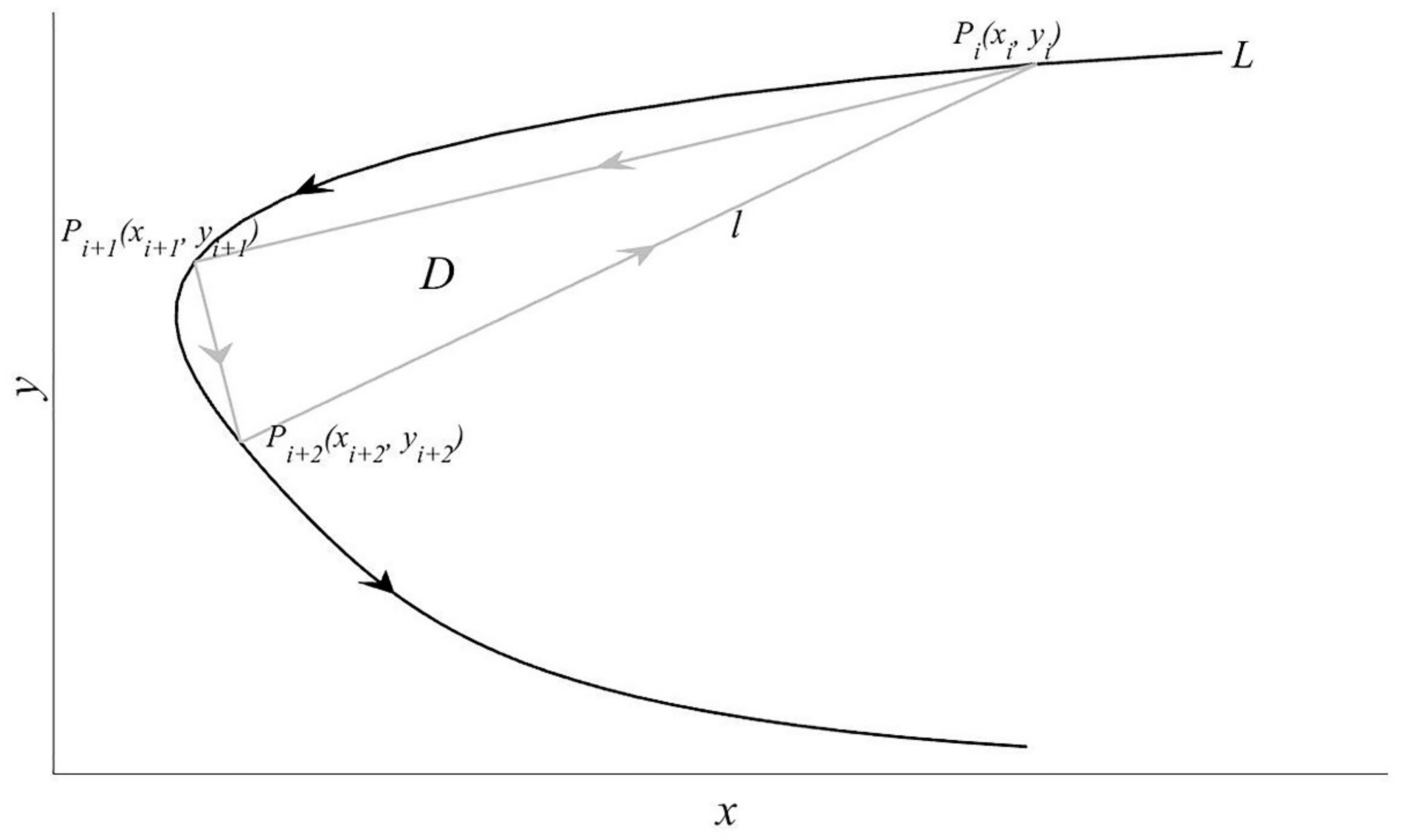
2.1. Abrupt Changes Based on Bifurcation Features

In the study of atmospheric motion, the optimal ordinary differential equations form the ideal atmospheric numerical model, but the dimension n is very high. Thus, the trajectories cannot be drawn in the normed linear space Rn, and so the Lorenz equations are taken as the research object. This is beneficial because, first, theoretical research can be carried out to obtain an abrupt change detection method based on the trajectory evolutions, and second, the Lorenz system is highly simplified, but qualitatively represents certain features of atmospheric dynamics. The Lorenz system comprises the following set of nonlinear equations:
d x d t = σ ( x + y ) d y d t = r x y x z d z d t = x y b z .
Here, x is the flipping velocity of convection, y is the temperature ratio, z is the temperature gradient in the vertical direction, σ is the Prandtl number, r is the relative Rayleigh number, and b is the velocity damping constant. When r is less than or equal to 1.0, there is only one equilibrium point at O(0,0,0)—this is the static state of the fluid. When r is greater than 1.0, there are three equilibrium points, namely, O(0,0,0), L ( b ( r 1 ) , b ( r 1 ) , r 1 ) , and R ( b ( r 1 ) , b ( r 1 ) , r 1 ) , where L and R denote left and right. In this case, the solution of the equation exhibits a bifurcation phenomenon. We take σ = 10, r = 28, and b = 8/3. By taking the initial position as (6, 20, 33) (or any other random value), numerical solutions of the dynamical system in Equation (1) can be determined using the four-rank Runge–Kutta algorithm with an incremental step of 0.001 over the integral interval [0, 50] and a truncation error of 0.013.
In Figure 1a, the black point is the left equilibrium point L and the blue point is the right equilibrium point R; the yellow curve is the trajectory of Lorenz Equation (1). One quasi-periodic trajectory (light gray bold segment) and one quasi-semi-periodic trajectory (light blue bold segment) are selected at random. The motion of these two sections of the trajectory is confined to one equilibrium point, representing the evolution of the solution of the dynamic system in one equilibrium region (the arrows indicate the direction of the trajectory). The green curve is a transition trajectory from the left equilibrium point region to the right equilibrium point region, and the pink curve is a transition trajectory from the right equilibrium region to the left equilibrium region. These two trajectories represent the transitions of the solution curves of the dynamical system between different equilibrium regions. The solution to the Lorenz Equation (1) changes significantly in the pink and green sections, demonstrating a kind of abrupt change. This abrupt change is caused by the bifurcation of Lorenz Equation (1), so it should have some physical meaning. For a dynamical system with more than two equilibrium points, the trajectory motion must have jump characteristics among the different equilibrium states. Therefore, these abrupt changes are relatively common, and can be defined as bifurcation-type abrupt changes. This type of abrupt change is the main focus of our study.
In Figure 1b, the horizontal direction is the time coordinate, and the curve is the y component of the light gray trajectory segment in Figure 1a. Figure 1c–e show the curves of the y component of the light blue, green, and pink trajectory segments in Figure 1a. Abrupt change detection can be applied to the time series in Figure 1b,c, and the abrupt change points are indicated by red stars. However, the time series in Figure 1d,e have no obvious characteristics of abrupt changes (of course, with different detection methods, there may be different detection results).
We can see from Figure 1a that the trajectory in the left equilibrium region rotates clockwise, whereas that in the right equilibrium region rotates counter-clockwise. Therefore, the rotation direction of the pink and green transition trajectories is bound to change. In view of these characteristics of the bifurcation-type abrupt change, we propose a method for their detection that is helpful in classifying and detecting abrupt changes in the atmosphere. It is also expected to provide a geometric and dynamic explanation for extreme weather events, such as abrupt changes between drought and flood in climate forecasts, and an early warning signal for abrupt climate change.

2.2. Bifurcation-Type Abrupt Change Detection Method

To determine the direction of a plane curve as either clockwise or counter-clockwise, consider the directional curve L in Figure 2. We select the points P 1 ( x 1 , y 1 ) , P 2 ( x 2 , y 2 ) , P 3 ( x 3 , y 3 ) , …, P n ( x n , y n ) on L in turn, and obtain the point sequence { P n ( x n , y n ) } . For different curves, we can adjust the density of the selected points. For the trajectory of a dynamical system, point sequence { P n ( x n , y n ) } can be taken as the numerical solution. The three vertices of triangle D in Figure 2 are P i ( x i , y i ) , P i + 1 ( x i + 1 , y i + 1 ) , and P i + 2 ( x i + 2 , y i + 2 ) ; these are enclosed by the directional line segments P i P i + 1 , P i + 1 P i + 2 , and P i + 2 P i , and the boundary of triangle D is l. We can write the integral of this curve as
S i 1 2 l x d y y d x = 1 2 ( p i p . i + 1 x d y y d x + p i + 1 p . i + 2 x d y y d x + p i + 2 p . i x d y y d x ) .
In the above formula, 1 2 l x d y y d x is the second type of curve integral on curve l, and the direction is indicated by the arrow. The geometrical meaning is the directed area of the triangle Δ P i P i + 1 P i + 2 . The integral can be obtained as
S i = 1 4 [ ( y i + 1 y i ) ( x i + x i + 1 ) ( x i + 1 x i ) ( y i + y i + 1 ) + ( y i + 2 y i + 1 ) ( x i + 1 + x i + 2 ) ( x i + 2 x i + 1 ) ( y i + 1 + y i + 2 ) ( y i + 2 y i ) ( x i + x i + 2 ) + ( x i + 2 x i ) ( y i + y i + 2 ) ] .
Simplifying this expression, we get
S i = 1 2 ( x i y i + 1 x i + 1 y i + x i + 1 y i + 2 x i + 2 y i + 1 x i y i + 2 + x i + 2 y i ) ,
where i = 1, 2, 3, …, n2 gives the series { S i } . The definition of the second type of curve integral states that if S i > 0 , the directional curve L is rotating counter-clockwise around the triangle Δ P i P i + 1 P i + 2 , and when S i < 0 , the directional curve L is rotating clockwise around the triangle Δ P i P i + 1 P i + 2 ; if S i = 0 , the curve is a straight line in the triangle Δ P i P i + 1 P i + 2 , that is, P i , P i + 1 , and P i + 2 are collinear. The direction of curve L can also be determined by the sign of the vector product of the following vectors:
p i p i + 1 = ( x i + 1 x i , y i + 1 y i )
p i + 1 p i + 2 = ( x i + 2 x i + 1 , y i + 2 y i + 1 ) .
If the vector product of p i p i + 1 and p i + 1 p i + 2 , i.e.,
p i p i + 1 × p i + 1 p i + 2 = x i + 1 y i + 2 x i y i + 2 + x i y i + 1 x i + 2 y i + 1 + x i + 2 y i + x i + 1 y i ,
is greater than zero, then L is rotating counter-clockwise; if the vector product is less than zero, L is rotating clockwise. Comparing Equations (4) and (6), they differ by a factor of two: this is obvious, because the vector product in Equation (6) is twice the area of the triangle Δ P i P i + 1 P i + 2 . We call the time series { S i } the area index time series, as the directional curve L is in the coordinate plane xoy. The area index time series is recorded as { S x o y i } .

2.3. Bifurcation-Type Abrupt Change Detection Test

For ease of exposition, the trajectory of the Lorenz equation in the region of the left equilibrium point is colored light gray and that in the right equilibrium region is colored light blue. The abrupt change points from the left equilibrium point area to the right equilibrium point area are marked with green points (curve segment), and the abrupt change points from the right equilibrium point area to the left equilibrium point area are marked with pink points (curve segment). This provision extends to the projection of the trajectory of the Lorenz equation on every coordinate plane.

2.3.1. Single-Index Time Series Abrupt Change Detection

Take the projection of the trajectory of Figure 1a on the coordinate plane xoz as the directional curve L, and consider the time interval [0, 10]. P 1 ( x 1 , z 1 ) , P 2 ( x 2 , z 2 ) , and P 3 ( x 3 , z 3 ) are taken on the curve L, where x 1 , x 2 , x 3 and z 1 , z 2 , z 3 are the x and z components of the numerical solution of Equation (1). According to Equation (4), we can obtain S x o z 1 , where the superscript xoz denotes that the curve is in the coordinate plane xoz and the subscript 1 indicates the first point; then, we take P 2 ( x 2 , z 2 ) , P 3 ( x 3 , z 3 ) , and P 4 ( x 4 , z 4 ) to obtain S x o z 2 , etc., to give the area index time series { S x o z i } . In Figure 3a, this area index time series is shown by the red line; the black line is the zero line, and the pink and green stars are the intersection points between the red curve and the black line. The pink stars (denoted as Tp2n1, Tp2n2, Tp2n3) indicate the points at which the time series { S x o z i } changes from positive to negative (the corresponding times are approximately 1.23, 3.63, and 9.39), while the green stars (denoted as Tn2p1 and Tn2p2) indicate the points at which { S x o z i } changes from negative to positive (the corresponding times are approximately 2.76 and 4.50). For convenience, Tp2n1 is also used to represent the time 1.23, and Tp2n2 is used to represent the time 3.63.
In the calculation of the numerical solution of Lorenz Equation (1), the integration step is 0.001. If we take the integration step to be 0.01, the length of the time series { S x o z i } is smaller, but we obtain similar results. Figure 3b shows the projection of the Lorenz trajectory in the xoz plane, where the light blue curve corresponds to S x o z i > 0 , the light gray curve corresponds to S x o z i < 0 , and the times corresponding to the pink stars are Tp2ni (i = 1,2,3) (note that two of these points are very close to each other, labeled as two). The times corresponding to the green stars are Tn2pj (j = 1,2). Figure 3c shows the trajectory of Lorenz Equation (1) in R3; the corresponding time intervals of every directed curve in the graph are exactly the same as in Figure 3b, and the corresponding times of the pink and green stars are also the same as in Figure 3b.
Figure 3b illustrates that when time series { S x o z i } is greater than zero, the trajectory rotates counter-clockwise in the region of the right equilibrium point; conversely, when the time series is less than zero, the trajectory rotates clockwise in the region of the left equilibrium point. There are two cases when { S x o z i } is equal to zero. At times Tp2ni (i = 1,2,3), the trajectory passes from the right equilibrium area to the left equilibrium area, while at times Tn2pj (j = 1,2), the trajectory passes from left to right. Figure 3c shows that the position of the trajectory can be determined by the positive and negative values of the time series { S x o z i } , that is, for S x o z i < 0 , the trajectory is in the left equilibrium region, and for S x o z i > 0 , the trajectory is in the right equilibrium region. However, when S x o z i = 0 , the trajectory transitions between the different equilibrium regions, and these are the times when the bifurcation-type abrupt changes occur.
We denote jumps from the right equilibrium region to the left equilibrium region as SCR2L; these correspond to the pink stars in Figure 3c and Tp2ni (i = 1,2,3). Jumps from the left equilibrium region to the right equilibrium region are defined as SCL2R; these correspond to the green stars in Figure 3c and Tn2pj (j = 1,2). We can see from Figure 3c that there are three instances of SCR2L and two instances of SCL2R in the time interval [0, 10]. Thus, our detection method did not produce any false or missed detections. This new method for detecting bifurcation-type abrupt changes is based on the dynamic characteristics of the Lorenz equation.
In conclusion, bifurcation-type abrupt changes occur when the time series { S x o z i } is equal to zero. Tp2ni correspond to SCR2L abrupt changes, and Tn2pj correspond to SCL2R abrupt changes.

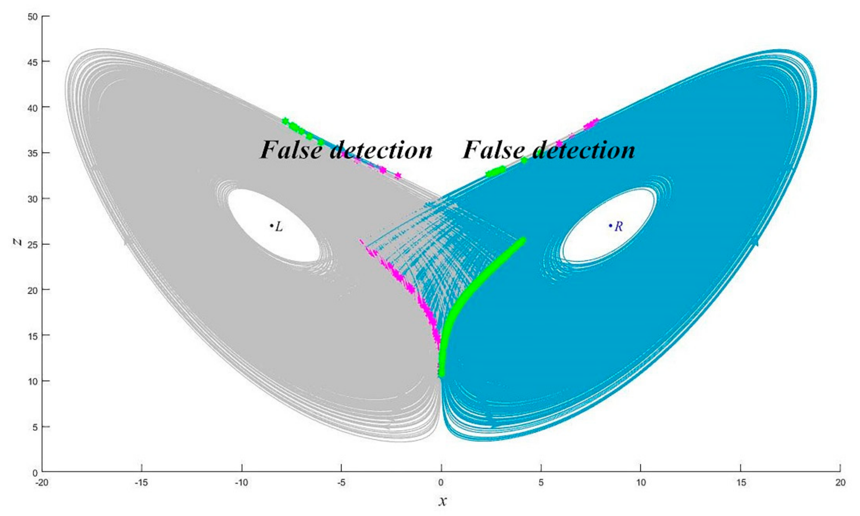
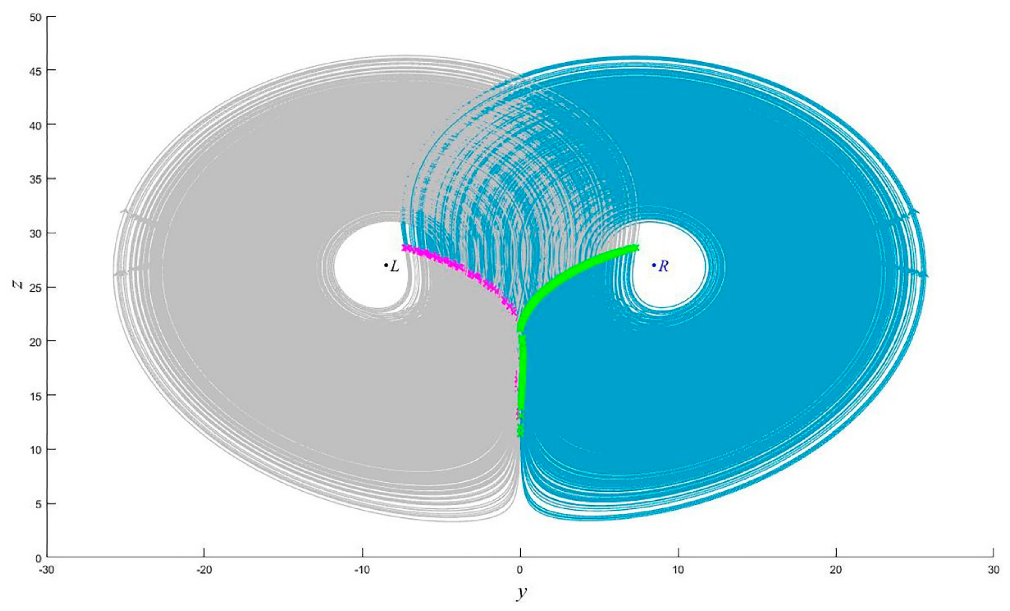
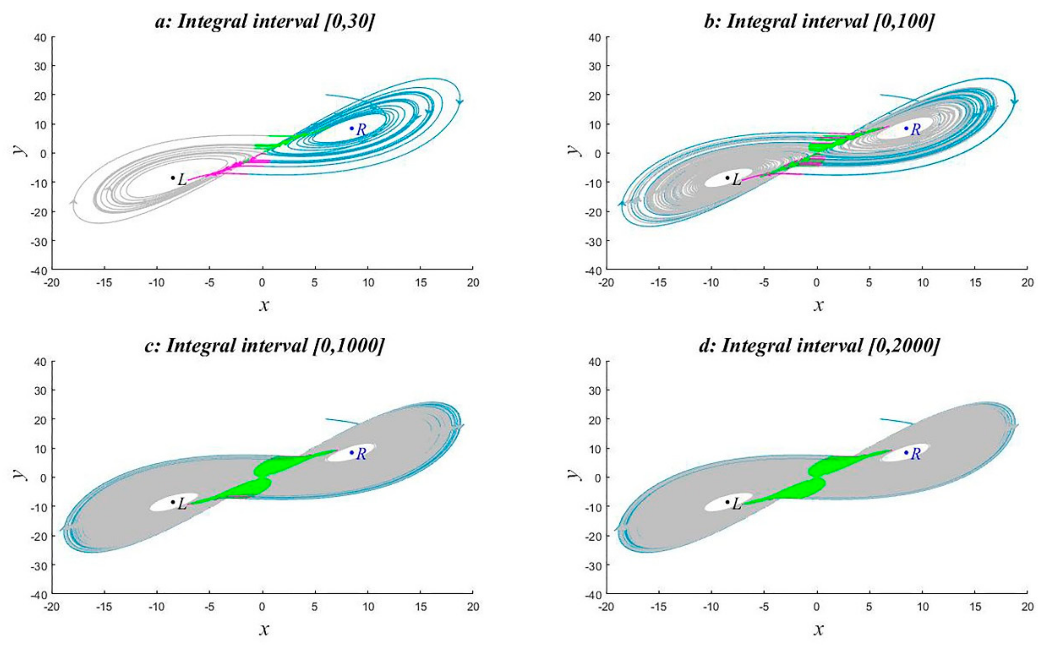
2.3.2. Multi-Index Time Series Abrupt Change Detection

The trajectory of Lorenz Equation (1) can be projected into the yoz and xoy coordinate planes to obtain two directional curves. According to Equation (4), time series { S y o z i } and { S x o y i } are obtained. { S x o z i } , { S y o z i } , and { S x o y i } are plotted in the same coordinate plane over the time interval [0, 10] in Figure 4. In this figure, the red curve is { S x o z i } , the purple curve is { S y o z i } , and the cyan curve is { S x o y i } ; the black line is the zero line, the pink regions correspond to the pink stars in Figure 3a, also identified by Tp2ni (i = 1,2,3), and the green regions correspond to the green stars in Figure 3a, also identified by Tn2pj (j = 1,2). The local map of the pink region Tp2n3 is given in the lower right corner.
The variation of the time series { S x o z i } has been analyzed above. { S y o z i } turns from positive to negative in the pink regions Tp2ni (i = 1,2,3), corresponding to times 1.13, 3.42, and 9.29, and turns from negative to positive in the green regions Tn2pj (j = 1,2), corresponding to times 2.65 and 4.43. It is positive in the intervals [0, 1.13], [2.65, 3.42], and [4.43, 9.29], and negative in the intervals [1.13, 2.65], [3.42, 4.43]. Time series { S x o y i } is slightly more complex. The series changes from negative to positive at times 1.14, 3.50, and 9.29 and changes from positive to negative at times 1.38, 3.95, and 9.54. Thus, in the pink transparent regions Tp2ni (i = 1,2,3), corresponding to time intervals [1.14, 1.38], [3.50, 3.95], and [9.29, 9.54], { S x o y i } is positive. In addition, the series changes from negative to positive at times 2.66 and 4.43 and from positive to negative at times 2.92 and 4.63. Thus, in green transparent regions Tn2pj (j = 1,2), corresponding to time intervals [2.66, 2.92] and [4.43, 4.63], { S x o y i } is also positive. At all other times, { S x o y i } is negative.
The following conclusions can be drawn: the time series { S x o z i } and { S y o z i } alternate between positive and negative, and the transitions are broadly synchronized. However, { S x o y i } is generally negative. The local map clearly shows that both { S x o z i } and { S y o z i } turn from positive to negative, but { S x o y i } turns from negative to positive, and then soon afterwards (about 0.2 time units later) turns back from positive to negative. The occurrence times of positive and negative transitions are largely in the time interval [9.28, 9.53]. The changes in the time series are similar in the remaining pink transparent region Tp2ni (i = 1,2). For the green transparent region Tn2pj (j = 1,2), there are similar results. The times at which { S y o z i } and { S x o z i } are equal to zero are not consistent within the same pink or green area, with { S y o z i } passing through zero slightly ahead of { S x o z i } .
To discuss the effect of abrupt change detection, we consider Figure 5. Figure 5a is the same as Figure 3b. Figure 5b is the projection of the trajectory of Lorenz Equation (1) onto the coordinate plane yoz. The direction and color of the trajectory are exactly the same as those in Figure 5a; however, every time interval is determined by the changes in the sign of the time series { S y o z i } . The points corresponding to the pink crosses in the figure are 1.13, 3.42, and 9.29, where S y o z i = 0 , and S y o z i turns from positive to negative. The points corresponding to the green crosses are 2.65 and 4.43, where S y o z i = 0 , and S y o z i turns from negative to positive. Figure 5c is the projection of the trajectory onto the coordinate plane xoy. As the initial field is in the right equilibrium region, the trajectory in interval [0, 1.14] is shown in light blue, the trajectory in interval [1.14, 1.38] is shown in pink, and the trajectory in interval [1.38, 2.66] is shown in light gray. That is, the trajectory color is determined by whether the time series { S x o y i } is positive or negative. The trajectory in R3 is shown in Figure 5, and the light blue and light gray trajectories are exactly the same as in Figure 3c. The positive and negative elements of the time series { S x o z i } are used to determine whether the trajectory is in the right or left equilibrium region. The times corresponding to the pink stars are when { S x o z i } is equal to zero in the pink areas in Figure 4, i.e., Tp2ni (i = 1,2,3), and the times corresponding to the green stars are when { S x o z i } is equal to zero in the green areas in Figure 4, i.e., Tn2pj (j = 1,2). The pink and green crosses indicate when the time series { S y o z i } is equal to zero. This is similar to the calibration method for the pink and green stars. The pink and green trajectories are determined by the time series { S x o y i } : the time intervals of the pink trajectory correspond to the pink area in Figure 4 when { S x o y i } is greater than zero, and the time intervals of the green trajectory correspond to the green area in Figure 4 when { S x o y i } is greater than zero. It is clear that the pink stars, crosses, and trajectories indicate jumps in the trajectory of the Lorenz equation from the right equilibrium region to the left equilibrium region. Similarly, the green stars, crosses, and trajectories indicate jumps in the trajectory of the Lorenz equation from the left equilibrium region to the right equilibrium region. Thus, the occurrence of bifurcation-type abrupt changes has been detected.
In summary, we can adopt the time at which the time series { S x o z i } or { S y o z i } is equal to zero as the occurrence time of a bifurcation-type abrupt change in Lorenz Equation (1), and can also judge the position of the trajectory from whether the time series { S x o z i } and { S y o z i } are positive or negative. This shows that when the rotation direction of the trajectory changes, there will be a bifurcation-type abrupt change. We can see that the time series { S y o z i } provides an early warning (i.e., the crosses are very prior to the stars) of an abrupt change, unlike { S x o z i } . Of course, this warning time scale is very small. If we consider the changes that occur over long time scales, this can be ignored. This also shows that the abrupt change time detected by different area index time series may be different, but it can be considered as within the range of error. As for why the abrupt change time is detected earlier or later in the different time series, we do not discuss this in detail here. Time series { S x o y i } can detect the abrupt change process, that is, the pink and green trajectory segments in Figure 5d, so we call these the transition trajectories.

2.3.3. Abrupt Change Detection Effect

Figure 5 shows that, as long as the abrupt change of trajectory can be detected in a certain coordinate plane, we can detect the abrupt change of trajectory in R3. We now consider the plane trajectory. First, we discuss the abrupt change detection using the time series { S x o z i } . Figure 6 gives the trajectory in the xoz plane over the time interval [0, 2000]. The curves and points are colored as in Figure 5a. There are seven blue tracks on the upper right side of the left equilibrium region, corresponding to the seven green stars and seven pink stars, and there are eight gray tracks on the upper left side of the right equilibrium region, corresponding to eight green stars and eight pink stars. Thus, this seems to indicate 30 abrupt changes, but these are actually false abrupt changes. The reasons for such false detections may be that the trajectories in these locations are close to straight lines, and when calculating the time series { S x o z i } , machine storage limitations and calculation errors may cause nonzero values to be calculated as zero values, giving a false detection. The abrupt change points are basically clustered on the pink and green star lines. There are 602 SCR2L abrupt changes and 601 SCL2R abrupt changes, with a false detection rate of 2.5%. Note that our method cannot determine whether there are any missed detections.
Figure 7 shows the abrupt change detection for the trajectory in the yoz plane given by time series { S y o z i } over the time interval [0, 2000]. Compared with Figure 6, time series { S y o z i } is more accurate in the detection of abrupt changes, and there are no false detections; again, we cannot comment on the possibility of missed detections.
Figure 8 shows the trajectory in the xoy plane for time intervals of [0, 30], [0, 100], [0, 1000], and [0, 2000]. The trajectory colors are consistent with those in Figure 5c. From Figure 8(a), the areas in which the trajectory dwells are easy to identify, and both SCR2L and SCL2R abrupt change processes can be detected (as shown by the pink and green trajectories in the figure). In Figure 8b, the SCR2L and SCL2R abrupt change processes are not easy to distinguish, and the position of the trajectory cannot be accurately determined. Similar conclusions can be reached for Figure 8c,d. The reason for this detection error is that the trajectory rotates clockwise in both the left and right equilibrium regions. Only in the green region in Figure 8 does it rotate counter-clockwise. Therefore, it is difficult to detect the position and abrupt change type, but the spatial location of the abrupt change must be in the green area in Figure 8d.

3. Conclusions and Implications

Based on the trajectories of the Lorenz equation, jumps among different equilibrium points have been defined as bifurcation-type abrupt changes. According to the rotation direction of the trajectories, a time series was constructed, and the positive and negative elements of the time series allowed us to determine the regions where the trajectory dwells. The points at which the time series are equal to zero are the moments when the trajectory jumps among different equilibrium regions, which determine the occurrence times of bifurcation-type abrupt changes. In conclusion, this method can accurately detect jumps within the Lorenz system of equations.
The motion of the atmosphere can be described by a set of partial differential equations, which can be discretized to give a set of ordinary differential equations. The atmosphere is also a dynamical system, so observation data or the output from numerical models can be regarded as the solution to this dynamical system, and the function image in the normed linear space Rn is the corresponding trajectory. The abrupt change detection method proposed in this paper has been applied to trajectories in the normed linear space R3; therefore, it can theoretically be used on trajectories in any normed linear space Rn. Consider the case in which T, u, v, w, p, and ρ denote time series of temperature, wind speed (three components of velocity), pressure, and density, respectively. The time series { S x o y i } associated with different meteorological elements can be constructed from Equation (4), where x and y are two of T, u, v, w, p, and ρ. By identifying the points at which the time series { S x o y i } is equal to zero, it is possible to determine the times at which abrupt climate changes occur. It is important to note that, although this method can theoretically be applied to climatic change, its application to real atmospheric data requires further investigation in the future. Once the dimension becomes very high, the discreteness of the observation data may cause some technical problems. In summary, the proposed abrupt change detection method has been established based on the dynamic significance of the system trajectories, and is able to detect abrupt changes in multi-dimensional time series.

Author Contributions

C.D. wrote the main text of the manuscript and undertook most of the theoretical research. B.S. wrote the introduction of the manuscript. J.S. translated the full text. B.S. and C.X. designed and implemented all numerical experiments. G.F. contributed to the scientific discussion. All authors have read and agreed to the published version of the manuscript.

Funding

This research is supported by the National Natural Science Foundation of China (Grant Nos. 41765004, 41530531 and 41875096), the National Key Research and Development Program of China (Grant No. 2017YFC1502303), and the National Social Science Foundation of China (Grant No 19VJX139).

Data Availability Statement

The data that support the findings of this study are in this paper.

Acknowledgments

We thank Stuart Jenkinson, from Liwen Bianji (Edanz) (www.liwenbianji.cn 17 June 2021) for editing the English text of a draft of this manuscript, and the Innovation Team of Intelligent Computing and Dynamical System Analysis and Application of Northwest Minzu University.

Conflicts of Interest

For both financial and non-financial interests, the authors declare no competing interests.

References

  1. Li, Q.; Wu, Z.; Wang, X.; Zhang, D.; Xiao, M. The Characteristics of Summer Precipitation in China since 1981 and its Relationship with SST and Pre-circulation. Plateau Meteorol. 2020, 39, 58–67. [Google Scholar]
  2. Yu, R.; Zhai, P. Ocean and cryosphere change related extreme events, abrupt change and its impact and risk. Clim. Chang. Res. 2020, 16, 194–202. [Google Scholar]
  3. Wang, G.; Lu, L.; Sun, J. Stability of Surrounding rock and Thrust Calculation of Shield Passing through Geological mediums. Chin. J. Rock Mech. Eng. 2015, 34, 2362–2372. [Google Scholar]
  4. Zeng, H.; Li, D.; Huang, H. Distribution Pattern of Ploidy Variation of Actinidia chinensis and A deliciosa. J. Wuhan Bot. Res. 2009, 27, 312–317. [Google Scholar]
  5. Zhao, X.; Zhou, B.; Li, Y. Application of T-DNA Insertion Mutagenesis in Functional Genomics of Plant. Lett. Biotechnol. 2009, 20, 880–884. [Google Scholar]
  6. Li, Z.; Zou, Y.; Jiang, Y.; Hu, Y.; Qin, Y.; Li, M.; Zhan, Y.; Wang, D.; Wang, N. Bioinformatics Analysis of Cap Protein Sequences of Porcine Circovirus Type. Lett. Biotechnol. 2020, 24, 13–20. [Google Scholar]
  7. Jin, C.; Zhao, Y. Progress in the study of KRAS mutation in lung adenocarcinoma. J. Int. Oncol. 2020, 47, 180–184. [Google Scholar]
  8. Gao, Z. Human capital, industrial structure mutation and economic catching up. China Mark. 2007, 40, 28–29. [Google Scholar]
  9. Liu, J. Social, Cultural and Psychological Factors of Network Language Variation. Xijiang Moon. 2013. Available online: https://xueshu.baidu.com/usercenter/paper/show?paperid=ee3b00947b1b20c4b9861fc83f709e7d&site=xueshu_se (accessed on 17 June 2021).
  10. Thom, R. Stabilité structurelle et morphogenèse. Poetics 1974, 3, 7–19. [Google Scholar] [CrossRef]
  11. Zeeman, E.C. Catastrophe Theory: A reply to Thom (Dynamical Systems-Warwick 1974); Springer: Berlin/Heidelberg, Germany, 1975; pp. 373–383. [Google Scholar]
  12. Daniell, P.J. Lectures on Cauchy’s Problem in Linear Partial Differential Equations by J Hadamard; Dover Publications: New York, NY, USA, 1953. [Google Scholar]
  13. Lorenz, E.N. Deterministic non-periodic flow. J. Atmos. Sci. 1963, 20, 130–141. [Google Scholar] [CrossRef] [Green Version]
  14. Fu, C.; Wang, Q. The definition and detection of the Abrupt Climatic Change. Chin. J. Atmos. Sci. 1992, 16, 15–21. [Google Scholar]
  15. Fu, C. Studies on the Observed Abrupt Climatic Change. Sci. Atmos. Sin. 1994, 18, 373–384. [Google Scholar]
  16. Zhu, K. East Asian monsoon and rainfall in China. Acta Geogr. Sinica. 1934, 1, 23–30. [Google Scholar]
  17. Tu, C.; Huang, T. Advance and retreat of summer monsoon in China. Acta Meteorol. Sin. 1944, 28, 234–247. [Google Scholar]
  18. Tao, S.; Chen, L. Structure of atmospheric circulation over Asian continent in summer. Chin. Sci. Bull. 1957, 7, 24–25. [Google Scholar]
  19. Ding, Y.; Zhang, L. Intercomparison of the time for climate abrupt change between the Tibetan Plateau and other regions in China. Chin. J. Atmos. Sci. 2008, 32, 794–805. [Google Scholar]
  20. Krishnamurti, T.N.; Ramanathan, Y. Sensitivity of the Monsoon Onset to Differential Heating. J. Atmos. Sci. 1979, 39, 1290–1306. [Google Scholar] [CrossRef] [Green Version]
  21. Shinoda, M.; Mikami, T.; Iwasaki, K.; Kitajima, H.; Eguchi, T.; Matsumoto, J.; Masuda, K. Global Simultaneity of the Abrupt Seasonal Changes in Precipitation during May and June of 1979. J Meteorol. Soc. Jpn. 1986, 64, 531–546. [Google Scholar] [CrossRef] [Green Version]
  22. Feng, G.; Gong, Z.; Dong, W.; Li, J. Abrupt climate change detection based on heuristic segmentation algorithm. Acta Phys. Sin. 2005, 54, 5494–5499. [Google Scholar]
  23. Hou, W.; Feng, G.; Dong, W.; Li, J. A technique for distinguishing dynamical species in the temperature time series of north China. Acta Phys. Sin. 2006, 53, 2663–2668. [Google Scholar]
  24. Gong, Z.; Feng, G.; Dong, W.; Li, J. The research of dynamic structure abrupt change of nonlinear time series. Acta Phys. Sin. 2006, 53, 3180–3187. [Google Scholar]
  25. Feng, G.; Gong, Z.; Zhi, R. Latest advances of climate change detecting technologies. Acta Meteorol. Sin. 2008, 66, 892–905. [Google Scholar]
  26. Zhi, R.; Gong, Z.; Wang, D.; Feng, G. Analysis of the spatio-temporal characteristics of precipitation of China based on the power-law exponent. Acta Phys. Sin. 2006, 53, 6185–6191. [Google Scholar]
  27. Huang, J.P.; Yi, Y.H.; Wang, S.W.; Chou, J.F. An analogue-dynamical long-range numerical weather prediction system incorporating historical evolution. Q. J. R. Meteorol. Soc. 1993, 119, 547–565. [Google Scholar]
  28. He, W.P.; Liu, Q.Q.; Gu, B.; Zhao, S.S. A novel method for detecting abrupt dynamic change based on the changing hurst exponent of spatial images. Clim. Dyn. 2016, 47, 2561–2571. [Google Scholar] [CrossRef]
  29. Halifa-Marín, A.; Lorente-Plazas, R.; Pravia-Sarabia, E.; Montávez, J.P.; Jiménez-Guerrero, P. Atlantic and mediterranean influence promoting an abrupt change in winter precipitation over the southern iberian peninsula. Atmos. Res. 2021, 253, 105485. [Google Scholar] [CrossRef]
  30. Guo, F.; Yan, M.; Zhang, K.; Lei, H.; Guo, L. The climate change in qingdao during 1899–2015 and its response to global warming. J. Geosci. Environ. Prot. 2018, 6, 58–70. [Google Scholar] [CrossRef] [Green Version]
  31. Rahman, M.R.; Lateh, H. Spatio-temporal analysis of warming in bangladesh using recent observed temperature data and GIS. Clim. Dyn. 2016, 46, 2943–2960. [Google Scholar] [CrossRef]
  32. Fang, S.; Yue, Q.; Han, G.; Li, Q.; Zhou, G. Changing trends and abrupt features of extreme temperature in mainland china from 1960 to 2010. Atmosphere 2016, 7, 22. [Google Scholar] [CrossRef] [Green Version]
Figure 1. Trajectory of the Lorenz equation and y component. (a) Trajectory of the Lorenz equation, (b) y component of one periodic trajectory, (c) y component of semi-periodic trajectory, (d) y component of transition trajectory from left equilibrium region to right equilibrium region, and (e) y component of transition trajectory from right equilibrium region to left equilibrium region.
Atmosphere 12 00781 g001
Figure 2. Diagram of curve integral.
Atmosphere 12 00781 g002
Figure 3. Area index time series and trajectory of the Lorenz equation. (a) Area index time series { S x o z i } (b) Trajectory of the Lorenz equation in coordinate plane xoz. (c) Trajectory of the Lorenz equation.
Atmosphere 12 00781 g003
Figure 4. Multiple area index time series.
Atmosphere 12 00781 g004
Figure 5. Trajectory of the Lorenz equation. (a) Trajectory in xoz coordinate plane. (b) Trajectory in yoz coordinate plane. (c) Trajectory in xoy coordinate plane. (d) Trajectory of the Lorenz equation.
Atmosphere 12 00781 g005
Figure 6. Trajectory of the Lorenz equation in xoz coordinate plane.
Atmosphere 12 00781 g006
Figure 7. Trajectory of the Lorenz equation in yoz coordinate plane.
Atmosphere 12 00781 g007
Figure 8. Trajectory of the Lorenz equation in xoy coordinate plane. (a) Integral interval [0, 30]. (b) Integral interval [0, 100]. (c) Integral interval [0, 1000]. (d) Integral interval [0, 2000].
Atmosphere 12 00781 g008
Publisher’s Note: MDPI stays neutral with regard to jurisdictional claims in published maps and institutional affiliations.

