Article

Non-Stationary Effects of the Arctic Oscillation and El Niño–Southern Oscillation on January Temperatures in Korea

1
Natural Science Research Institute, Gangneung-Wonju National University, Gangneung 25457, Korea
2
Department of Atmospheric and Environmental Sciences, Gangneung-Wonju National University, Gangneung 25457, Korea
3
Department of Atmospheric Science, Kongju National University, Gongju 32588, Korea
4
Department of Mathematics and Statistics, Chonnam National University, Gwangju 61186, Korea
5
Department of Earth Science Education, Kyungpook National University, Daegu 41566, Korea
6
National Institute of Meteorological Sciences, Seogwipo 63568, Korea
*
Author to whom correspondence should be addressed.
Atmosphere 2021, 12(5), 538; https://doi.org/10.3390/atmos12050538
Submission received: 25 March 2021 / Revised: 19 April 2021 / Accepted: 20 April 2021 / Published: 22 April 2021

Abstract

:
In recent decades, extremely cold winters have occurred repeatedly throughout the Northern Hemisphere, including the Korean Peninsula (hereafter, Korea). Typically, cold winter temperatures in Korea can be linked to the strengthening of the Siberian High (SH). Although previous studies have investigated the typical relationship between the SH and winter temperatures in Korea, this study uniquely focused on a change in the relationship, which reflects the influence of the Arctic Oscillation (AO) and El Niño–Southern Oscillation (ENSO). A significant change in the 15-year moving correlation between the SH and the surface air temperature average in Korea (K-tas) was observed in January. The correlation changed from −0.80 during 1971–1990 to −0.16 during 1991–2010. The mean sea-level pressure pattern regressed with the temperature, and a singular value decomposition analysis that incorporated the temperature and pressure supports that the negative high correlation during 1971–1990 was largely affected by AO. This connection with AO is substantiated by empirical orthogonal function (EOF) analysis with an upper-level geopotential height at 300 hPa. In the second mode of the EOF, the temperature and pressure patterns were primarily affected by ENSO during 1991–2010. Consequently, the interdecadal change in correlation between K-tas and the SH in January can be attributed to the dominant effect of AO from 1971–1990 and of ENSO from 1991–2010. Our results suggest that the relative importance of these factors in terms of the January climate in Korea has changed on a multidecadal scale.

1. Introduction

Unlike the globally decreasing long-term trend in the frequency and intensity of cold surges, record-breaking cold events have increased in Northern Hemisphere middle latitudes in recent decades [1]. These cold events, which have concurrently occurred with Arctic warming and sea-ice melting resulting from anthropogenic global warming, have been termed “Warm Arctic, Cold Continents” (WACC) [2]. It is widely accepted that the WACC pattern occurs as a consequence of a decrease in the meridional temperature gradient owing to global warming and polar amplification; the weakening of the polar vortex has induced intensification of the meridional component of large-scale atmospheric flows that bring the cold continental air from high latitudes to middle latitudes [3]. In addition to the WACC pattern, cold extremes under global warming have been investigated in many studies, especially in middle-latitude areas [2,4,5,6,7].
It has also been suggested that cold continents in the WACC pattern are affected by low-frequency atmospheric variability rather than by Arctic warming [8], which implies that the WACC pattern could be transient instead of a persistent change. This pattern suggested the possibility of affecting the Arctic climate from the solar cycle [9]. Ural blocking associated with Arctic sea ice loss also appeared to affect cold events on the Asian continent [10,11,12]. Oceanic variabilities with a multi-decadal time scale (e.g. Atlantic multidecadal oscillation), not just atmospheric factors, can also play an important role in inducing cold wave events in mid-latitudes of the Northern Hemisphere [13,14,15,16].
The purpose of this study was to understand the mechanism of cold extremes on the Korean Peninsula (hereafter, Korea). Traditionally, cold extremes in East Asia, including Korea, have been related to a change in the strength and degree of extension of the Siberian High (SH) [17,18]. This study investigated the relationship between the SH and the surface air temperature average in Korea in January. However, unlike previous studies that investigated the typical relationship between the SH and the winter temperature in Korea, this study uniquely focused on the change in the relationship and the mechanism behind this change.
In addition to the SH, several other factors have been investigated to explain the mechanisms of cold extremes in East Asia. Variability in Arctic Oscillation (AO) affects the winter temperature change in Eurasia and has been associated with a change in the strength of SH [19,20] in an opposite phase during 1972–1977 and 1987–1995 [21]. A study discussed that there was a shift in Northern Hemisphere circulation pattern before and after 1976. From 1976 to 1996 there were differences in many regional teleconnection patterns [22]. A recent study demonstrates that the relationship between AO and surface air temperature over Korea for the boreal winter season is not static but changes on the decadal time scale [23]. In addition to the AO, the El Niño–Southern Oscillation (ENSO) affects wintertime temperatures in East Asia.
Being closely related to the East Asia winter temperature, the East Asian winter monsoon (EAWM) and its relationship with Ural–Siberia blocking is also influenced by AO and ENSO, especially through their combined effects, which vary with time [24,25]. Some previous studies have mentioned that the relationship of the EAWM with AO and ENSO both experienced significant interdecadal changes (e.g., [26,27,28]). After 1979, the correlation of the first mode of the empirical orthogonal function (EOF) for EAWM with ENSO was weakened, whereas the correlation of the second mode for EAWM with AO was strengthened [29]. A weakening of both EAWM and SH is correlated with a positive phase of North Pacific Oscillation (NPO), and the inverse is true (strengthening correlated with a negative phase) [26,28,30]. A regime shift in EAWM was reported in association with a change in large-scale circulation patterns [30,31,32,33,34]. The interdecadal variability of the EAWM after the mid-1980s and its possible causes has also been examined [29,34,35,36]. In an analysis using the fifth phase of the Coupled Model Intercomparison Project (CMIP5) simulation data, the relationships between EAWM and each of ENSO and AO were projected to seesaw in the 21st century; this did not appear in historical simulation data [37]. However, most of these previous studies focused on the non-stationary effects of AO and ENSO on a continental scale wintertime climate.
The objective of this study was to examine the multidecadal impact of the non-stationary effects of AO and ENSO on a local scale (the Korean Peninsula) wintertime temperature. The change in the relationship between the surface air temperature averaged over Korea and the strength of SH is explained by the changing influence of large-scale patterns including AO and ENSO. The data and analysis methods used for this study are described in Section 2. In Section 3, we show that the relationship between the cold extremes in Korea and the strength of SH has changed between two different periods during recent decades. Subsequently, to determine the physical reason for the change in the relationship, a composite analysis of the large-scale flow surrounding Korea is presented. Finally, in Section 4, the conclusions are drawn along with a discussion of the results.

2. Data and Methods

The main dataset used in this study was the National Center for Environmental Prediction/National Center for Atmospheric Research (NCEP/NCAR) reanalysis [38] from 1949–2017 with a horizontal resolution of 2.5° × 2.5°. The monthly mean anomaly time series of surface air temperature, mean sea-level pressure and geopotential height at 300 h Pa were used to investigate the relationship between winter cold temperature in Korea and SH and the underlying mechanism for the relationship change between the periods of 1971–1990 (hereafter, P1) and 1991–2010 (hereafter, P2). This interdecadal change in the relationship was determined with a 15-year moving correlation coefficients time series in January between the monthly mean surface air temperature average for Korea (hereafter, K-tas) and an index for the strength of the Siberian High (SHI). The daily mean temperature was exclusively used to formulate a cumulative distribution function to test if a temperature was statistically distinguishable between the two periods.
The focus of the study was K-tas, defined as the surface air temperature in January averaged over the area 34°–43° N and 124°–131° E, including the Korean Peninsula. Based on the typical relationship of winter temperature in Korea with the strength of the SH, our analysis focused on their correlation over time. The strength of SH was determined from the SHI, which is defined as the mean sea-level pressure anomaly averaged over the region of 40°–60° N and 80°–120° E [39].
To examine the underlying mechanisms for the change in correlation between K-tas and SHI, the large-scale flow surrounding Korea was analyzed in terms of mean sea-level pressure, which can be characterized in the regions with the AO index as defined by [40], the index of Aleutian Low Intensity (ALI) as defined by [41], and the ENSO index. However, the Nino3.4 index was used to represent ENSO in the subsequent analysis. The Nino3.4 index, defined as the anomaly of sea surface temperature averaged over the area of 5° S–5° N and 120°–170° W, is computed by using the ERSSTv5 (Extended Reconstructed Sea Surface Temperature version 5) dataset [42]. In addition to the climate variability indices, the climatological means in the two periods were compared for surface air temperature and mean sea-level pressure. A multivariate analysis tool called singular value decomposition (SVD) [43] was also applied to the temperature and pressure. In addition to the large-scale flow at the surface level, the geopotential height at 300 hPa was analyzed using EOF to examine the upper-level change in the flow.

3. Results

3.1. Correlation between the Winter Temperature in Korea and SH

The time series of the K-tas and SHI are presented for January along with their correlation coefficients using a 15-year moving window (Figure 1). The mean of the correlation coefficients for the entire period is −0.55, indicating that an increase in SHI would lead to increasingly severe winter temperatures in Korea [17,44,45,46].
Notably, the correlation coefficients considerably vary with time, showing a maximum of −0.86 in 1984 and a minimum of −0.04 in 2000. The moving correlation coefficients of the time series appeared to be recurrent, with a period of approximately 40 years; however, the data length was too short to affirm this observation. In contrast, we focused on the period centered approximately on the year 1990, when there was a remarkable change in the correlation: P1 from 1971 to 1990 and P2 from 1991 to 2010. During P1, the correlation coefficient was −0.80, meaning that the January temperature in Korea was closely related to SHI. During P2, the coefficient was −0.16, indicating that the contribution of SH to the temperature in Korea became insignificant. It is worth mentioning the reason why we paid attention only to January. We found that the correlation coefficient between K-tas and SHI is quite different each month in winter. The correlation for January decreases significantly from P1 to P2, whereas the correlation for December and February increase slightly (not shown here). As the result, the correlation for the winter averaged (DJF average) appears to decrease slightly. So, we decided to focus our interest only on January.
Figure 2 presents a map of the correlation coefficient between K-tas and the anomaly of mean sea-level pressure calculated at each grid point. Overall, the correlation was negative over the middle latitude continental area, thereby ensuring a traditional perspective that winter temperatures in Korea are influenced by the dry and cold air divergent from the SH in the north [17,44,47]. Positive correlation over the North Pacific was also notable, and this may have bought warm and humid air to Korea along the border of the Aleutian Low. The correlation pattern during P1 and P2 resembled the negative and positive patterns of the AO, respectively. In the following sub-sections, more in-depth analyses are used to explain this AO-like correlation pattern and the change from P1 to P2. Related to the winter temperatures in Korea, a negative AO event can have a significant influence on SH [19,20,21]. However, when interpreting such a correlation map, we must be cautious that the opposite correlations over SH and the Aleutian Low do not necessarily affect the temperature simultaneously. However, the significant correlations over the regions certainly influenced the winter temperature in Korea during these periods, especially in P1 with higher correlations.
Figure 2 confirms that the considerably lower correlation between K-tas and SHI during P2, as shown in Figure 1, resulted from a weakening of the correlation between K-tas and the pressure anomaly, rather than from a cancellation effect between the positive and negative correlation regions (Figure 2b). The positive and negative peaks in the correlation maps were reduced from −0.82 and 0.72 during P1 to −0.55 and 0.46 during P2.

3.2. Time-Mean Anomaly Pattern of Temperature and Mean Sea-Level Pressure

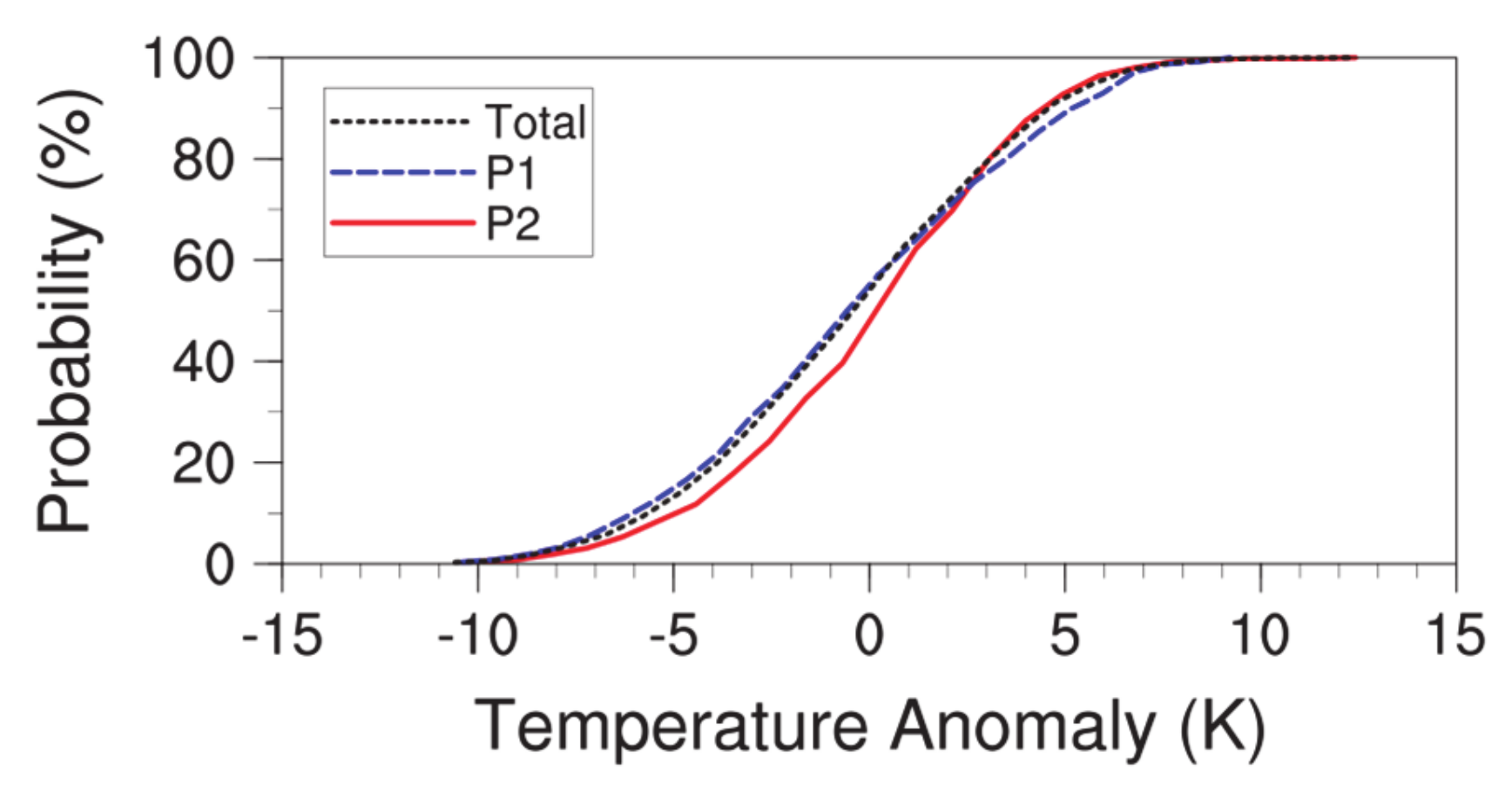
The change in correlation between K-tas and SHI may have also changed the winter climate in Korea. To determine if the time series of the temperature averaged over Korea were distinctive from each other for the two periods, a Kolmogorov–Smirnov test was conducted following [48], as shown in Figure 3, in which the cumulative distribution function of the average daily mean surface air temperature anomalies for Korea are presented. To eliminate global warming effects, the temperature anomalies were detrended beforehand. The test resulted in the distribution function for the period P1 being different from that for the period P2 at a significance level of 0.01; however, the former was statistically identical to that for the entire period, although it did not meet the significance level of 0.05. The distribution functions obtained for the analysis periods indicated that the winter in P1 was certainly colder than the winter in P2, which supports the theory that a higher negative correlation of K-tas with SH may bring increasingly severe cold weather to Korea.
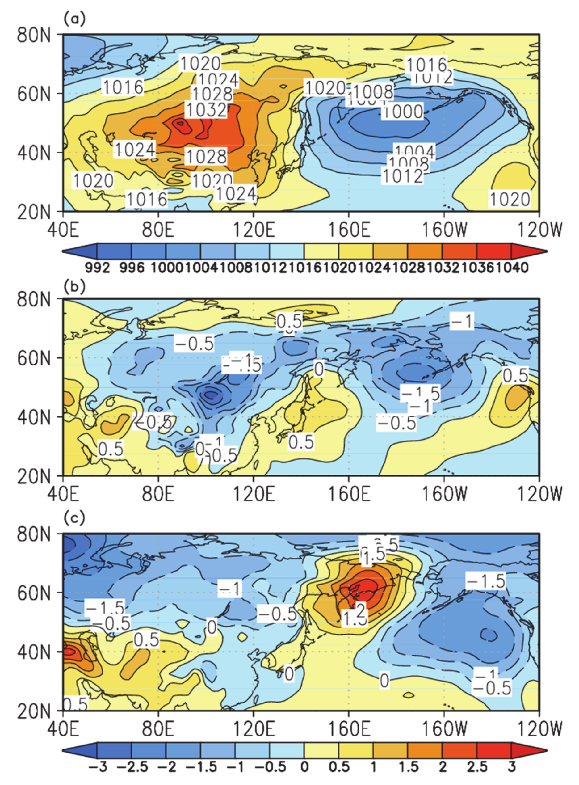
The cold winter in P1 with the high correlation between K-tas and SHI was spread throughout large parts of the Asian continent, except for mainland China (Figure 4b), and it became colder than climatology (Figure 4a). During P2 with the low correlation, the winter climate was warmer in most areas of Asia, including Korea, compared with the winter in P1, as well as to the normal state throughout the entire period [6,34]. These temperature changes in Asia during the periods contradicted the global warming rate, as this rate was the highest during P1 in the 20th century but was the lowest during P2, the period also known as “the global warming hiatus” (1998–2012) [5,7]. These contradictory results suggest that the January temperature in Korea during these periods may have been influenced by regional factors, one of which may have been a change in the correlation between K-tas and SHI instead of global warming.
During P1, the SH was weakened and the Aleutian Low was strengthened, as represented by the negative anomaly in Figure 5b. During P2, the SH was also weakened, but the change was not significant. In contrast, the negative anomaly over the Arctic Ocean peaking over the Barents Sea and the positive anomaly over the Bering Sea displayed the opposite pattern of the temperature anomaly (Figure 4c).
These pressure and temperature anomaly patterns are not in accordance with the correlation pattern in Figure 2. Thus, they are insufficient to explain the correlation change between the two periods. Consequently, the time-mean distributions of temperature and mean sea-level pressure anomalies were not necessarily consistent with the correlation map for the anomalies.

3.3. Large-Scale Circulation around Korea

3.3.1. Surface Air Temperature and Mean Sea-Level Pressure

To determine the reason for the correlation change between the two periods, spatial and temporal variations for the surface air temperature in Korea and the mean sea-level pressure in Asia were analyzed simultaneously using a singular value decomposition (SVD); the results are shown in Figure 6. Notably, the pressure pattern of the first mode resembles the correlation map of opposite phases for the two periods. The first mode’s contribution to the total variability was 98.5% in P1 and 88.0% in P2. The correlation coefficient between the principal component time series for the temperature anomaly in Korea and the pressure anomaly in Asia was also reduced from 0.82 in P1 to 0.56 in P2.
Although a cold tongue of air was elongated to the south during P1 and brought a severe cold event to the Korean Peninsula, this phenomenon was flattened during P2, resulting in a warmer winter. The cold tongue during P1 appeared to have occurred owing to the continental high from the north over the Asian continent being confronted with a marine low that developed over the middle-latitude North Pacific. During P2, the continental high moved to the northwest and the marine low became weaker. Although the continental high and marine low here are decomposed components in the SVD analysis, they contribute to most of the total variability and can be considered as anomaly patterns of the SH and the Aleutian Low, respectively. Subsequently, the reduction in the correlation between K-tas and SHI can be attributed to a shift of the SH to the northwest. However, it is unclear how the shift in the SH was related to the weakening of the Aleutian Low during P2.
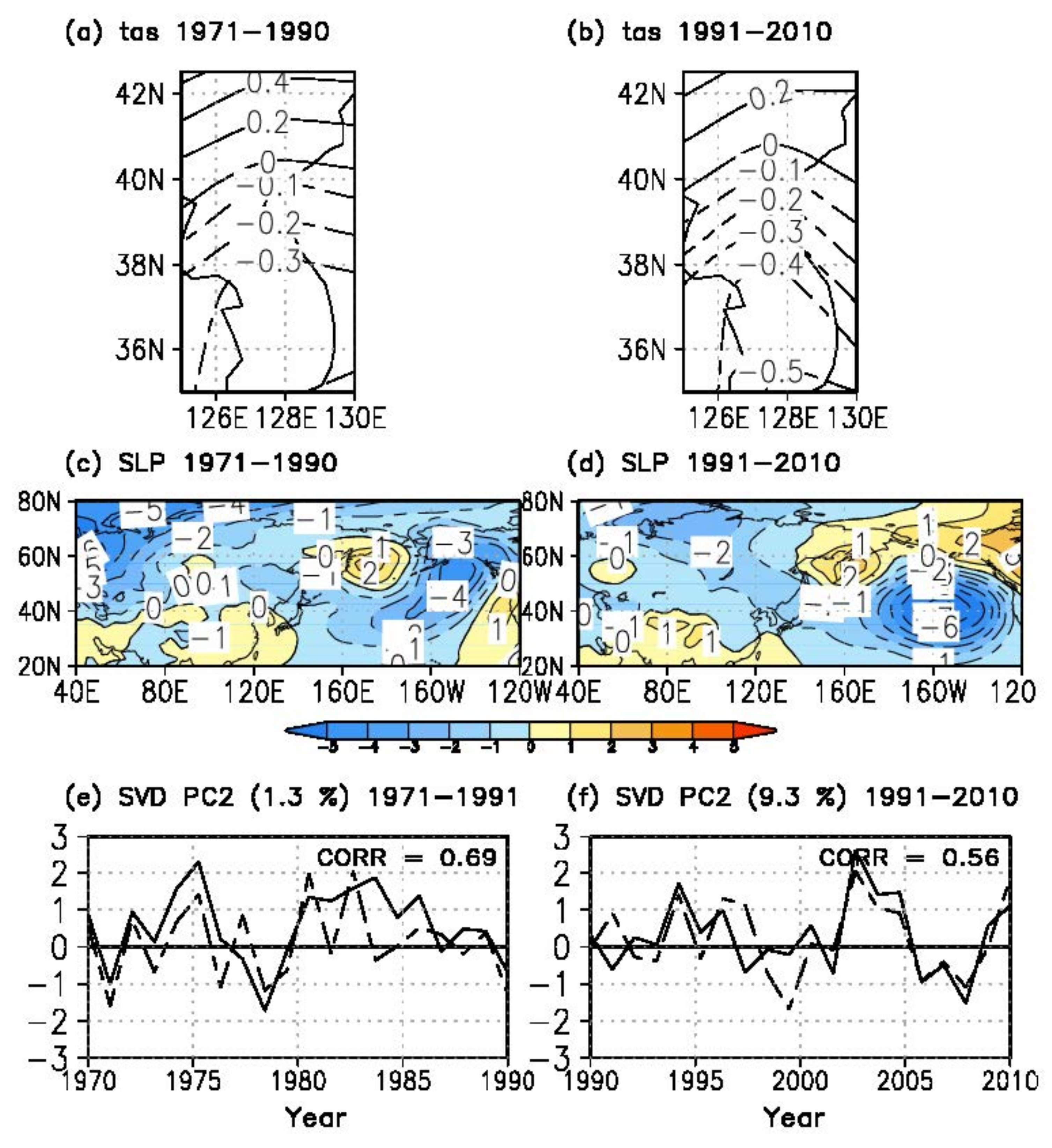
Unlike the first mode, the second modes resulting from the SVD analysis for P1 and P2 were similar, and their principal component time series revealed the same correlation coefficient of 0.7 (Figure 7). Although their contribution to the total variability changed from 1.3% in P1 to 9.3% in P2, based on the similarity in the second mode, the first mode was the primary reason for the change in correlation between K-tas and SHI.
Table 1 and Table 2 compare the correlations between the AO and Nino3.4 indices and the SHI and ALI. The correlation of SHI with AO considerably reduced from −0.43 in P1 to −0.03 in P2, and the correlation of ALI with Nino3.4 significantly intensified from −0.31 in P1 to −0.70 in P2; this confirms that the relative importance of the factors affecting winter climate in Korea changed during these periods. Consequently, the interdecadal change in correlation between the surface air temperature in Korea and the mean sea level pressure in January can be attributed to the stronger effects of AO during 1971–1990 and ENSO during 1991–2010.

3.3.2. Geopotential Height at 300 hPa

In addition to the cold spells in East Asia, including Korea, that resulted from the development and expansion of SHI [17,18], an upper-level wave train and blocking high have recently been attributed to extreme cold weather in Korea [45,46]. Thus, the geopotential height at 300 h Pa was analyzed with EOF.
In Figure 8, the first mode in P1 and P2 resembles the AO pattern known as the opposite phases of the air pressure anomaly between the Arctic region and the middle latitudes [49]. The first mode’s contribution to the total variability was 36% in P1 and 26% in P2, which was similar to the contribution change of the first mode of mean sea-level pressure in the SVD analysis with surface air temperature (Figure 6).
The second mode in P1 appears to be related to the NPO [30], known as the second EOF mode of the mean sea-level pressure. During P2, the Aleutian Low was dominant. This change in the pattern over the North Pacific between the two periods is consistent with a previous study, in that the southern lobe of the NPO pattern has shifted eastward since 1990 in association with ENSO [50]. These upper-level patterns in P1 and P2 shown in the second EOF mode reveal two distinct features in the North Pacific: mean sea-level pressure anomalies forced by North Pacific Gyre Oscillation (NPGO), resulting in NPO and Pacific Decadal Oscillation (PDO) [51] associated with variability in ENSO [52], resulting in a strengthening of the Aleutian Low.
To confirm that the results of EOF analysis with the geopotential height at 300 h Pa can be explained by surface-level features, the correlations of the geopotential height with AO and Nino3.4 indices are shown in Figure 9. Remarkably, the correlation map with the AO index is similar to the first mode eigenvector for both periods (Figure 8a), whereas the correlation map with the Nino3.4 index is similar to the second mode eigenvector.
The highest positive correlation occurred over the Northwest Pacific coast near the Korean Peninsula, with a correlation coefficient of 0.74 for P1 and 0.73 for P2 (Figure 9a,b). Based on the correlation between the surface air temperature in Korea and the mean sea level pressure displaying a typical AO pattern (Figure 2), this result suggests that the winter temperature in Korea is highly affected by AO from the surface level to this upper level at 300 h Pa. The pressure pattern of negative AO in P1 is especially known to cause the intensification of a blocking high over the Ural Mountains in January [7], followed by the development of an atmospheric trough over East Asia [19] that can bring cold air inflow from the polar region to middle-latitude areas including Korea.
The correlation with the Nino3.4 index peaked with a negative maximum at the Aleutian Low over the North Pacific showing correlation coefficients at −0.61 in P1 and −0.77 in P2 (Figure 9c,d). The stronger correlation over the region in P2 was consistent with the Aleutian Low having been strengthened during El Niño events in boreal winter [53].

4. Summary and Conclusions

In this study, the correlation between the average surface air temperature in Korea and the SHI considerably changed from −0.8 during 1971–1990 to −0.16 during 1991–2010. Both the mean sea-level pressure pattern regressed to the temperature and SVD analysis with the temperature and the pressure supports that the high negative correlation during 1971–1990 was largely affected by AO through its interdecadal change. During this period, the SH and Aleutian Low were strengthened with an expansion to middle latitudes. Cold air from the north along the strengthened SH brought severe cold to Korea more frequently; this is a typical causality of extreme cold events in this region. However, even if the Siberian High does not develop, there is a possibility that extremely cold winters have occurred repeatedly throughout the Northern Hemisphere, including the Korean Peninsula. This connection with AO was validated by the EOF analysis with an upper-level geopotential height at 300 h Pa.
EOF analysis results provide additional insights into winter temperature and pressure patterns in Korea during 1991–2010; specifically, they were most affected by the ENSO through teleconnection from low latitudes. During this period, the January temperature was warmer than that during P1.
Although there have been studies that have investigated the influences of AO and ENSO on the winter climate in Korea, this study uniquely focused on the change in the factors determining the winter temperature by means of moving correlation. The changes in the two periods may have resulted from multidecadal variations related to AO and ENSO or their combination. In the future, it will be necessary to reveal more underlying mechanisms of the non-stationary effects of AO and ENSO. To do so, we require simulations using a sophisticated climate model with proper experimental design, along with the analysis of more long-term observational datasets.

Author Contributions

Conceptualization, J.-S.Y., H.-J.S. and I.-U.C.; methodology, I.-U.C., M.-K.K., J.-S.P. and D.-S.R.P.; software, J.-S.Y., K.-Y.J. and H.-J.S.; validation, M.-K.K., Y.-H.B., K.-O.B. and I.-U.C.; investigation, J.-S.Y., H.-J.S., K.-Y.J. and I.-U.C.; data curation, J.-S.Y., K.-Y.J., Y.-H.B., K.-O.B. and H.-M.S.; writing—original draft preparation, J.-S.Y., H.-J.S. and I.-U.C.; writing—review and editing, J.-S.Y., H.-J.S. and I.-U.C.; visualization, J.-S.Y. and K.-Y.J.; supervision, Y.-H.B., K.-O.B. and M.-K.K.; project administration, Y.-H.B., K.-O.B. and H.-M.S.; funding acquisition, I.-U.C., M.-K.K., J.-S.P., D.-S.R.P., Y.-H.B., K.-O.B. and H.-M.S. All authors have read and agreed to the published version of the manuscript.

Funding

This work was supported by the Korea Meteorological Administration Research and Development Program under grant number KMI2018-03410. Work of the NIMS/KMA authors was performed under the auspices of the Korea Meteorological Administration Research and Development Program “Development and Assessment of IPCC AR6 Climate Change Scenarios (KMA2018-00321)”. H-J. Shin was also supported by the National Research Foundation of Korea (NRF) and the Center for Women in Science, Engineering and Technology (WISET; grant number 2018-072) funded by the Ministry of Science and ICT (MSIT) under the Program for Returners into R&D.

Institutional Review Board Statement

Not applicable.

Informed Consent Statement

Not applicable.

Data Availability Statement

All data is publicly available via the National Oceanic and Atmospheric Administration (NOAA) Physical Sciences Laboratory website (https://psl.noaa.gov/data/gridded/index.html) (last access: 15 March 2021).

Acknowledgments

We appreciate the two anonymous reviewers for their valuable suggestions and questions.

Conflicts of Interest

The authors declare no conflict of interest.

References

  1. Lu, C.; Xie, S.; Qin, Y.; Zhou, J. Recent Intensified Winter Coldness in the Mid-High Latitudes of Eurasia and Its Relationship with Daily Extreme Low Temperature Variability. Adv. Meteorol. 2016, 2016, 17–19. [Google Scholar] [CrossRef] [Green Version]
  2. Overland, J.E.; Wood, K.R.; Wang, M. Warm Arctic-cold continents: Climate impacts of the newly open arctic sea. Polar Res. 2011, 30. [Google Scholar] [CrossRef]
  3. Francis, J.; Skific, N. Evidence linking rapid Arctic warming to mid-latitude weather patterns. Philos. Trans. A Math. Phys. Eng. Sci. 2015, 373. [Google Scholar] [CrossRef]
  4. Cohen, J.; Pfeiffer, K.; Francis, J.A. Warm Arctic episodes linked with increased frequency of extreme winter weather in the United States. Nat. Commun. 2018, 9, 1–12. [Google Scholar] [CrossRef] [PubMed]
  5. Johnson, N.C.; Xie, S.P.; Kosaka, Y.; Li, X. Increasing occurrence of cold and warm extremes during the recent global warming slowdown. Nat. Commun. 2018, 9, 4–6. [Google Scholar] [CrossRef] [PubMed] [Green Version]
  6. Kim, Y.H.; Kim, M.K.; Lau, W.K.M.; Kim, K.M.; Cho, C.H. Possible mechanism of abrupt jump in winter surface air temperature in the late 1980s over the Northern Hemisphere. J. Geophys. Res. 2015, 120, 12474–12485. [Google Scholar] [CrossRef] [PubMed]
  7. Li, C.; Stevens, B.; Marotzke, J. Eurasian winter cooling in the warming hiatus of 1998–2012. Geophys. Res. Lett. 2015, 42, 8131–8139. [Google Scholar] [CrossRef] [Green Version]
  8. Sun, L.; Perlwitz, J.; Hoerling, M. What caused the recent “Warm Arctic, Cold Continents” trend pattern in winter temperatures? Geophys. Res. Lett. 2016, 43, 5345–5352. [Google Scholar] [CrossRef]
  9. Roy, I. Solar cyclic variability can modulate winter Arctic climate. Sci. Rep. 2018, 8, 1–15. [Google Scholar] [CrossRef]
  10. Cohen, J.; Jones, J.; Furtado, J.C.; Tziperman, E. Warm Arctic, cold continents a common pattern related to Arctic sea ice melt, snow advance, and extreme winter weather. Oceanography 2013, 26, 150–160. [Google Scholar] [CrossRef]
  11. Luo, D.; Xiao, Y.; Diao, Y.; Dai, A.; Franzke, C.L.E.; Simmonds, I. Impact of Ural blocking on winter warm Arctic-cold Eurasian anomalies. Part II: The link to the North Atlantic Oscillation. J. Clim. 2016, 29, 3949–3971. [Google Scholar] [CrossRef]
  12. Xu, X.; He, S.; Li, F.; Wang, H. Impact of northern Eurasian snow cover in autumn on the warm Arctic–cold Eurasia pattern during the following January and its linkage to stationary planetary waves. Clim. Dyn. 2018, 50, 1993–2006. [Google Scholar] [CrossRef]
  13. Cao, Y.; Liang, S.; Yu, M. Observed low-frequency linkage between Northern Hemisphere tropical expansion and polar vortex weakening from 1979 to 2012. Atmos. Res. 2020, 243, 105034. [Google Scholar] [CrossRef]
  14. Shi, J.; Cui, L.; Ma, Y.; Du, H.; Wen, K. Trends in temperature extremes and their association with circulation patterns in China during 1961–2015. Atmos. Res. 2018, 212, 259–272. [Google Scholar] [CrossRef]
  15. Sung, M.K.; Kim, S.H.; Kim, B.M.; Choi, Y.S. Interdecadal variability of the warm Arctic and cold Eurasia pattern and its North Atlantic origin. J. Clim. 2018, 31, 5793–5810. [Google Scholar] [CrossRef]
  16. Yu, L.; Zhong, S.; Sui, C.; Sun, B. Revisiting the trend in the occurrences of the warm Arctic-cold Eurasian continent temperature pattern. Atmos. Chem. Phys. 2020, 1–48. [Google Scholar] [CrossRef]
  17. Jhun, J.G.; Lee, E.J. A new East Asian winter monsoon index and associated characteristics of the winter monsoon. J. Clim. 2004, 17, 711–726. [Google Scholar] [CrossRef]
  18. Zhang, Y.; Sperber, K.R.; Boyle, J.S. Climatology and Interannual Variation of the East Asian Winter Monsoon: Results from the 1979–95 NCEP/NCAR Reanalysis. Mon. Weather Rev. 1997, 125, 2605–2619. [Google Scholar] [CrossRef]
  19. Gong, D.Y.; Ho, C.H. The Siberian High and climate change over middle to high latitude Asia. Theor. Appl. Climatol. 2002, 72, 1–9. [Google Scholar] [CrossRef]
  20. Gong, D.Y.; Wang, S.W.; Zhu, J.H. East Asian winter monsoon and Arctic Oscillation. Geophys. Res. Lett. 2001, 28, 2073–2076. [Google Scholar] [CrossRef]
  21. Wu, B.; Wang, J. Winter Arctic Oscillation, Siberian High and East Asian Winter Monsoon. Geophys. Res. Lett. 2002, 29, 3–6. [Google Scholar] [CrossRef]
  22. Roy, I. Addressing on Abrupt Global Warming, Warming Trend Slowdown and Related Features in Recent Decades. Front. Earth Sci. 2018, 6, 1–19. [Google Scholar] [CrossRef]
  23. Jun, Y.; Song, K.; Son, S. Decadal Changes in the Relationship between Arctic Oscillation and Surface Air Temperature over Korea. Atmosphere 2021, 31, 61–71. [Google Scholar]
  24. Chen, W.; Lan, X.Q.; Wang, L.; Ma, Y. The combined effects of the ENSO and the Arctic Oscillation on the winter climate anomalies in East Asia. Chinese Sci. Bull. 2013, 58, 1355–1362. [Google Scholar] [CrossRef] [Green Version]
  25. Cheung, H.N.; Zhou, W.; Mok, H.Y.; Wu, M.C. Relationship between Ural-Siberian Blocking and the East Asian winter monsoon in relation to the Arctic oscillation and the El Niño-Southern Oscillation. J. Clim. 2012, 25, 4242–4257. [Google Scholar] [CrossRef]
  26. Wang, L.; Chen, W.; Huang, R. Interdecadal modulation of PDO on the impact of ENSO on the east Asian winter monsoon. Geophys. Res. Lett. 2008, 35, 1–4. [Google Scholar] [CrossRef] [Green Version]
  27. Gong, H.; Wang, L.; Chen, W. Multidecadal changes in the influence of the arctic oscillation on the east asian surface air temperature in boreal winter. Atmosphere 2019, 10, 757. [Google Scholar] [CrossRef] [Green Version]
  28. Gong, H.; Wang, L.; Chen, W. Recently strengthened influence of ENSO on the Wintertime East Asian surface air temperature. Atmosphere 2019, 10, 720. [Google Scholar] [CrossRef] [Green Version]
  29. Yun, K.S.; Seo, Y.W.; Ha, K.J.; Lee, J.Y.; Kajikawa, Y. Interdecadal changes in the Asian winter monsoon variability and its relationship with ENSO and AO. Asia-Pacific J. Atmos. Sci. 2014, 50, 531–540. [Google Scholar] [CrossRef]
  30. Yun, J.; Ha, K.J.; Jo, Y.H. Interdecadal changes in winter surface air temperature over East Asia and their possible causes. Clim. Dyn. 2017, 51, 1375–1390. [Google Scholar] [CrossRef]
  31. Chen, S.; Song, L. Recent strengthened impact of the winter Arctic Oscillation on the Southeast Asian surface air temperature variation. Atmosphere 2019, 10, 164. [Google Scholar] [CrossRef] [Green Version]
  32. He, S. Reduction of the East Asian winter monsoon interannual variability after the mid-1980s and possible cause. Chinese Sci. Bull. 2013, 58, 1331–1338. [Google Scholar] [CrossRef] [Green Version]
  33. Kim, J.W.; An, S. Il; Jun, S.Y.; Park, H.J.; Yeh, S.W. ENSO and East Asian winter monsoon relationship modulation associated with the anomalous northwest Pacific anticyclone. Clim. Dyn. 2017, 49, 1157–1179. [Google Scholar] [CrossRef]
  34. Lee, S.S.; Kim, S.H.; Jhun, J.G.; Ha, K.J.; Seo, Y.W. Robust warming over East Asia during the boreal winter monsoon and its possible causes. Environ. Res. Lett. 2013, 8. [Google Scholar] [CrossRef]
  35. Wang, H.J.; He, S.P. Weakening relationship between East Asian winter monsoon and ENSO after mid-1970s. Chin. Sci. Bull. 2012, 57, 3535–3540. [Google Scholar] [CrossRef] [Green Version]
  36. Yang, L.N.; Wu, B.Y. Interdecadal variations of the East Asian winter surface air temperature and possible causes. Chin. Sci. Bull. 2013, 58, 3969–3977. [Google Scholar] [CrossRef] [Green Version]
  37. Wang, H.; He, S.; Liu, J. Present and future relationship between the East Asian winter monsoon and ENSO: Results of CMIP5. J. Geophys. Res. Ocean. 2013, 118, 5222–5237. [Google Scholar] [CrossRef] [Green Version]
  38. Kalnay, E.; Collins, W.; Deaven, D.; Gandin, L.; Iredell, M.; Jenne, R.; Joseph, D. The NCEP_NCAR 40-year reanalysis project. 1996.pdf. Bull. Am. Meteorol. Soc. 1996, 77, 437–472. [Google Scholar] [CrossRef] [Green Version]
  39. Lee, H.S.; Jhun, J.G. Two types of a Asian continental blocking and their relation to the east Asian monsoon during the boreal winter. Geophys. Res. Lett. 2006, 33, 1–5. [Google Scholar] [CrossRef]
  40. Thompson, D.W.J.; Wallace, J.M. The Arctic oscillation signature in the wintertime geopotential height and temperature fields. Geophys. Res. Lett. 1998, 25, 1297–1300. [Google Scholar] [CrossRef] [Green Version]
  41. Trenberth, K.E.; Hurrell, J.W. Decadal atmosphere-ocean variations in the Pacific. Clim. Dyn. 1994, 9, 303–319. [Google Scholar] [CrossRef]
  42. Trenberth, K.E. The Definition of El Niño. Bull. Am. Meteorol. Soc. 1997, 78, 2771–2777. [Google Scholar] [CrossRef] [Green Version]
  43. Venegas, S.A.; Mysak, L.A.; Straub, D.N. Atmosphere-ocean coupled variability in the South Atlantic. J. Clim. 1997, 10, 2904–2920. [Google Scholar] [CrossRef]
  44. Jeong, Y.K.; Renwick, J.A. Locations of the Siberian high centers of action and associated propagation of wave-like patterns in the northern hemisphere winter. Asia Pac. J. Atmos. Sci. 2008, 44, 149–171. [Google Scholar]
  45. Park, T.W.; Ho, C.H.; Deng, Y. A synoptic and dynamical characterization of wave-train and blocking cold surge over East Asia. Clim. Dyn. 2014, 43, 753–770. [Google Scholar] [CrossRef]
  46. Park, T.-W.; Ho, C.-H.; Jeong, J.-H.; Heo, J.-W.; Deng, Y. A new dynamical index for classification of cold surge types over East Asia. Clim. Dyn. 2015, 45, 2469–2484. [Google Scholar] [CrossRef]
  47. Huang, W.; Wang, B.; Wright, J.S.; Chen, R. On the Non-Stationary Relationship between the Siberian High and Arctic Oscillation. PLoS ONE 2016, 11, e0158122. [Google Scholar] [CrossRef]
  48. Dosio, A.; Fischer, E.M. Will Half a Degree Make a Difference? Robust Projections of Indices of Mean and Extreme Climate in Europe Under 1.5°C, 2°C, and 3°C Global Warming. Geophys. Res. Lett. 2018, 45, 935–944. [Google Scholar] [CrossRef] [Green Version]
  49. Thompson, D.W.J.; Wallace, J.M. Annular modes in the extratropical circulation. Part I: Month-to-month variability. J. Clim. 2000, 13, 1000–1016. [Google Scholar] [CrossRef]
  50. Yeh, S.W.; Yi, D.W.; Sung, M.K.; Kim, Y.H. An Eastward Shift of the North Pacific Oscillation After the mid-1990s and Its Relationship with ENSO. Geophys. Res. Lett. 2018, 45, 6654–6660. [Google Scholar] [CrossRef]
  51. Chhak, K.; Di Lorenzo, E. Decadal variations in the California Current upwelling cells. Geophys. Res. Lett. 2007, 34, 1–6. [Google Scholar] [CrossRef] [Green Version]
  52. Linkin, M.E.; Nigam, S. The North Pacific Oscillation-West Pacific teleconnection pattern: Mature-phase structure and winter impacts. J. Clim. 2008, 21, 1979–1997. [Google Scholar] [CrossRef]
  53. Papineau, J.M. Wintertime temperature anomalies in Alaska correlated with ENSO and PDO. Int. J. Climatol. 2001, 21, 1577–1592. [Google Scholar] [CrossRef]
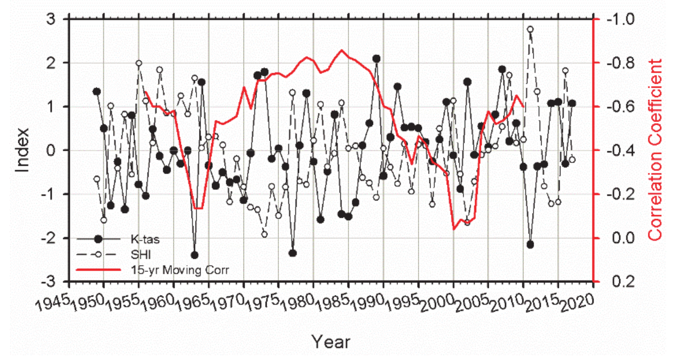
Figure 1. Time series of normalized indices forming surface air temperature averaged for Korea (K-tas) (black solid line with circles), and the strength of Siberian High (SHI) (black dashed line with open circles) in January from 1949 to 2017 calculated with NCEP/NCAR reanalysis data. The red line, labeled on the right-hand side of the figure, denotes the correlation coefficients between K-tas and SHI with 15-year moving window indices.
Atmosphere 12 00538 g001
Figure 2. Correlation between the surface air temperature averaged over Korea and the mean sea-level pressure anomaly at each grid point, calculated for January of (a) 1971–1990 and (b) 1991–2010. The green dots denote statistical significance with a 95% confidence interval.
Atmosphere 12 00538 g002
Figure 3. Cumulative distribution function of the detrended daily surface air temperature anomalies (K) averaged for Korea in January from 1949 to 2017 (black dotted line) and two analysis periods divided by the correlation between the temperature time series and SHI: P1 for 1971–1990 with a high correlation (blue dashed line), and P2 for 1991–2010 with a low correlation (red solid line).
Atmosphere 12 00538 g003
Figure 4. NCEP/NCAR reanalysis: (a) surface air temperature in January averaged for 1949–2017, as well as (b) anomalies for 1971–1990, and (c) 1991–2010. The unit of temperature used here is K.
Atmosphere 12 00538 g004
Figure 5. Same as Figure 4, except for mean sea-level pressure. (a) 1949–2017, (b) 1971–1990 and (c) 1991–2010. The unit of the mean sea-level pressure is hPa.
Atmosphere 12 00538 g005
Figure 6. (a,b) The first mode of SVD analysis with the surface air temperature anomaly, (c,d) mean sea-level pressure anomaly and (e,f) their principal component time series. The left panels present the results for the period from 1971 to 1990 and the right panels present the period from 1990 to 2010. At the bottom, dashed lines denote the results for the temperature and solid lines for the pressure. NCEP/NCAR reanalysis data for January mean were used for the analysis.
Atmosphere 12 00538 g006
Figure 7. Same as Figure 6, except for the second mode of SVD. (a,b) surface air temperature, (c,d) mean sea-level pressure and (e,f) their principal component time series.
Atmosphere 12 00538 g007
Figure 8. Eigenvectors of the first and second EOF modes of the geopotential height at 300 hPa, obtained with January means from NCEP/NCAR reanalysis for (a,c) 1971–1990 and (b,d) 1991–2010.
Atmosphere 12 00538 g008
Figure 9. Correlation map of the 300 hPa geopotential high anomaly based on the (top) AO index and (bottom) ENSO index in January. (a,b) 1971–1990, (c,d) 1991–2010. The green dots denote 95% confidence.
Atmosphere 12 00538 g009
Table 1. Correlation coefficient between SHI and the AO as well as Nino3.4 indices. (*) denotes statistical significance at the 95% significance level.
SHIAONino3.4
1949–2017−0.33 *0.02
1971–1990−0.430.13
1991–2010−0.03−0.17
Table 2. Same as Table 1, except for ALI.
ALIAONino3.4
1949–20170.33 *−0.46 *
1971–19900.40−0.31
1991–20100.43−0.70 *
Publisher’s Note: MDPI stays neutral with regard to jurisdictional claims in published maps and institutional affiliations.