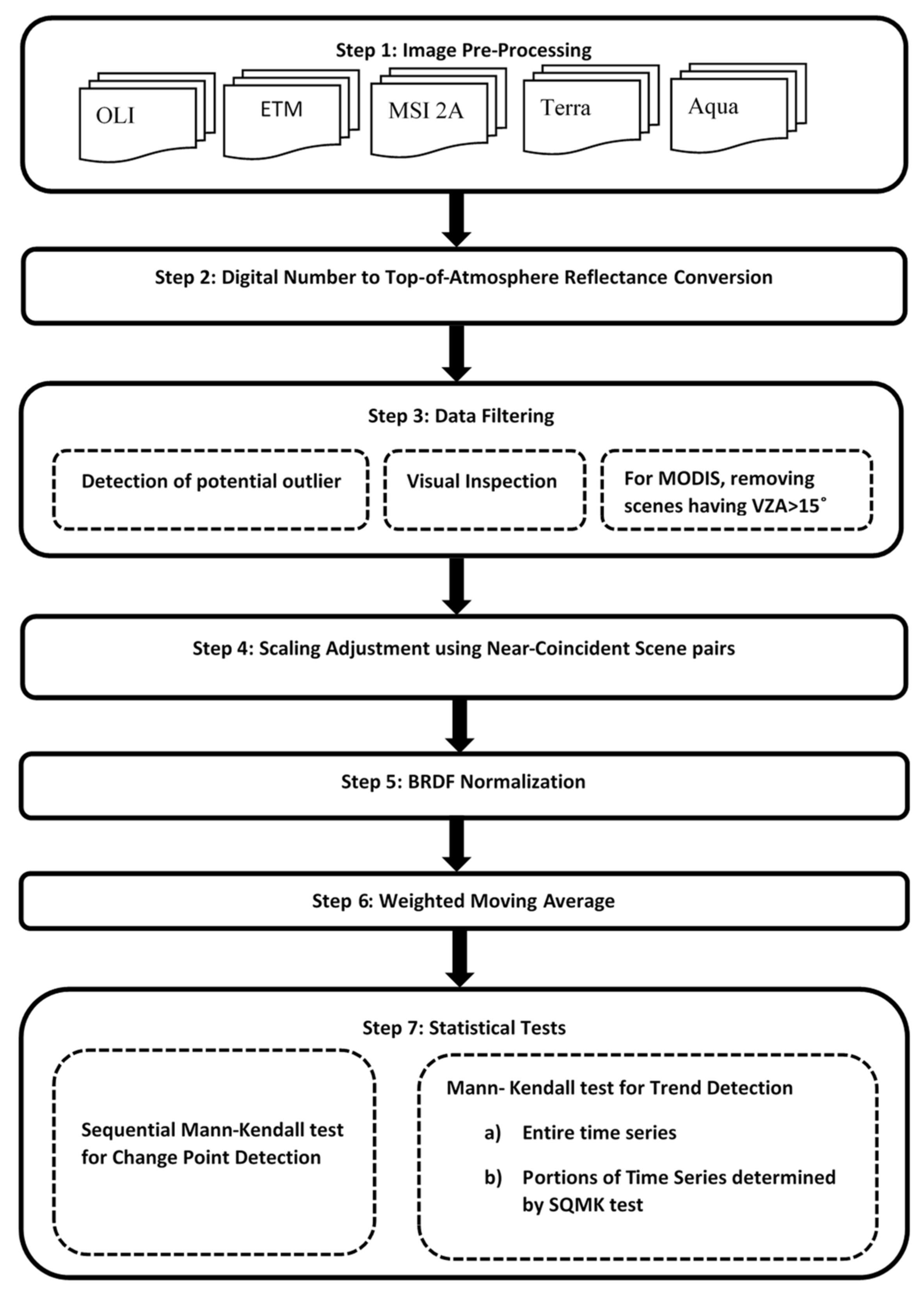
Figure 1.
General flowchart for change point detection of PICS. VZA is the View Zenith Angle; BRDF is Bidirectional Reflectance Distribution Function; SQMK is Sequential Mann–Kendall.
Figure 1.
General flowchart for change point detection of PICS. VZA is the View Zenith Angle; BRDF is Bidirectional Reflectance Distribution Function; SQMK is Sequential Mann–Kendall.
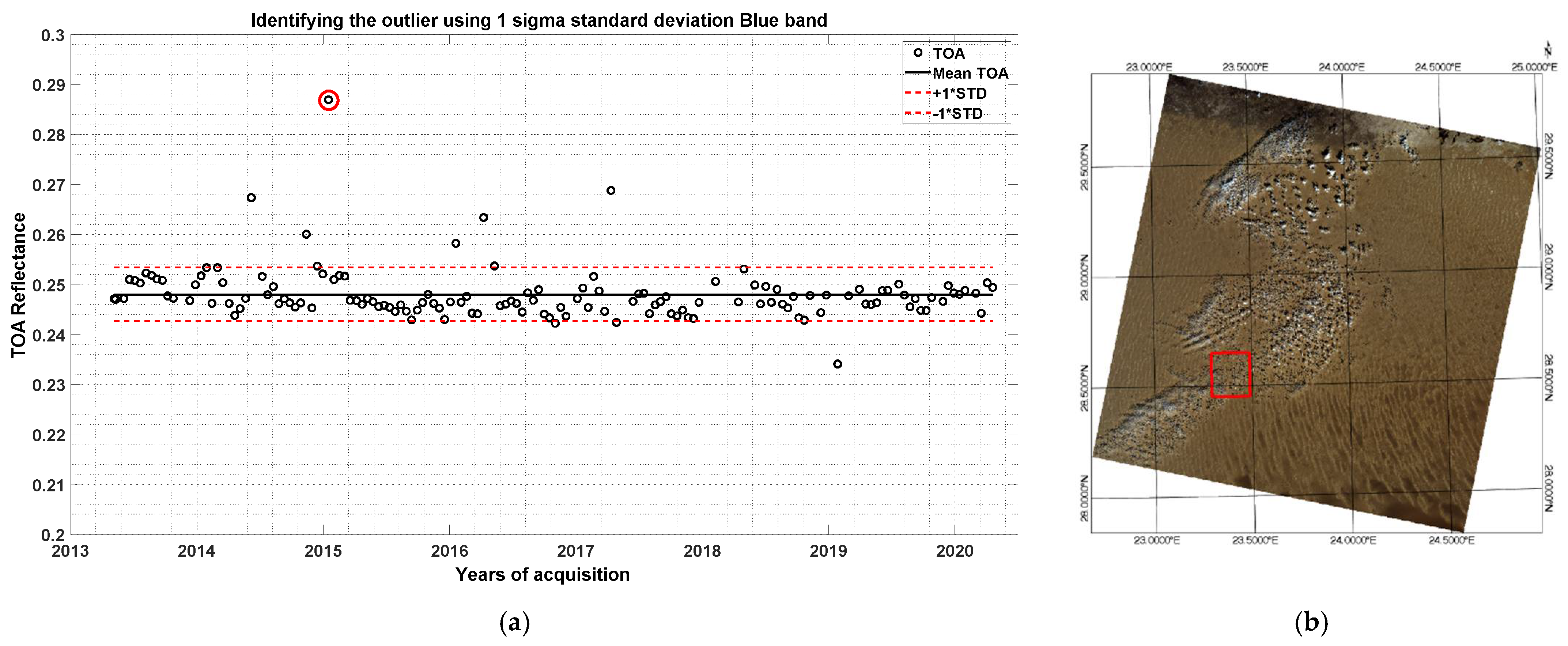
Figure 2.
(a) Graph to illustrate the identification of outlier using 2-sigma standard deviation method; and (b) visual inspection of the image considered as a potential outlier.
Figure 2.
(a) Graph to illustrate the identification of outlier using 2-sigma standard deviation method; and (b) visual inspection of the image considered as a potential outlier.
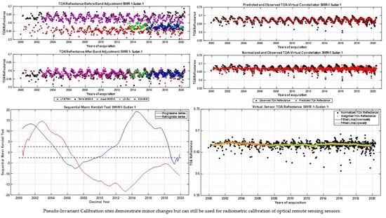
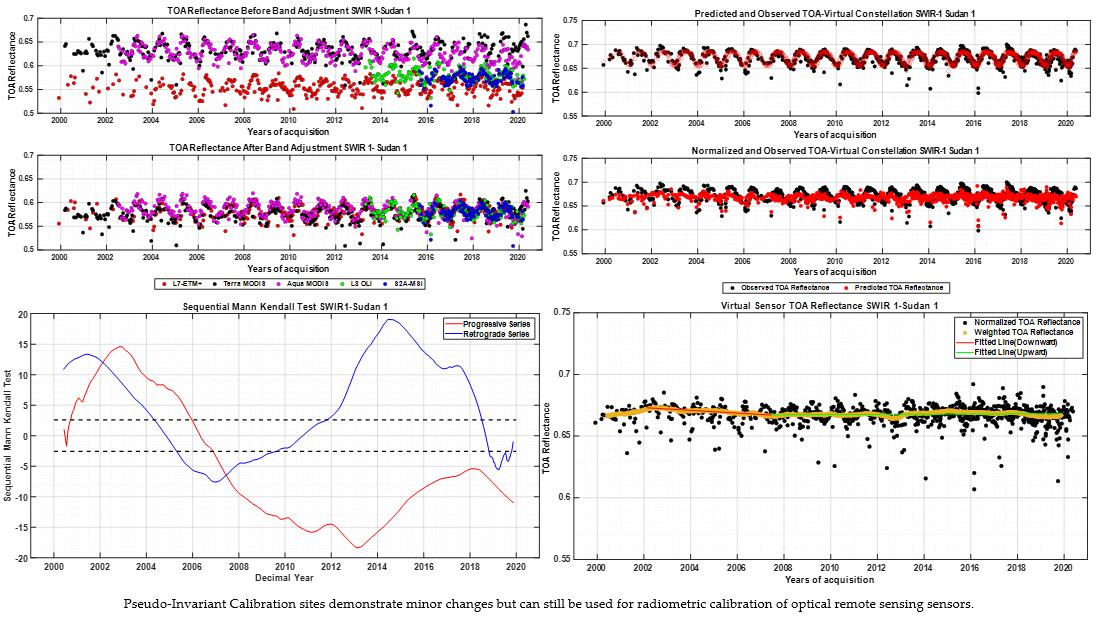
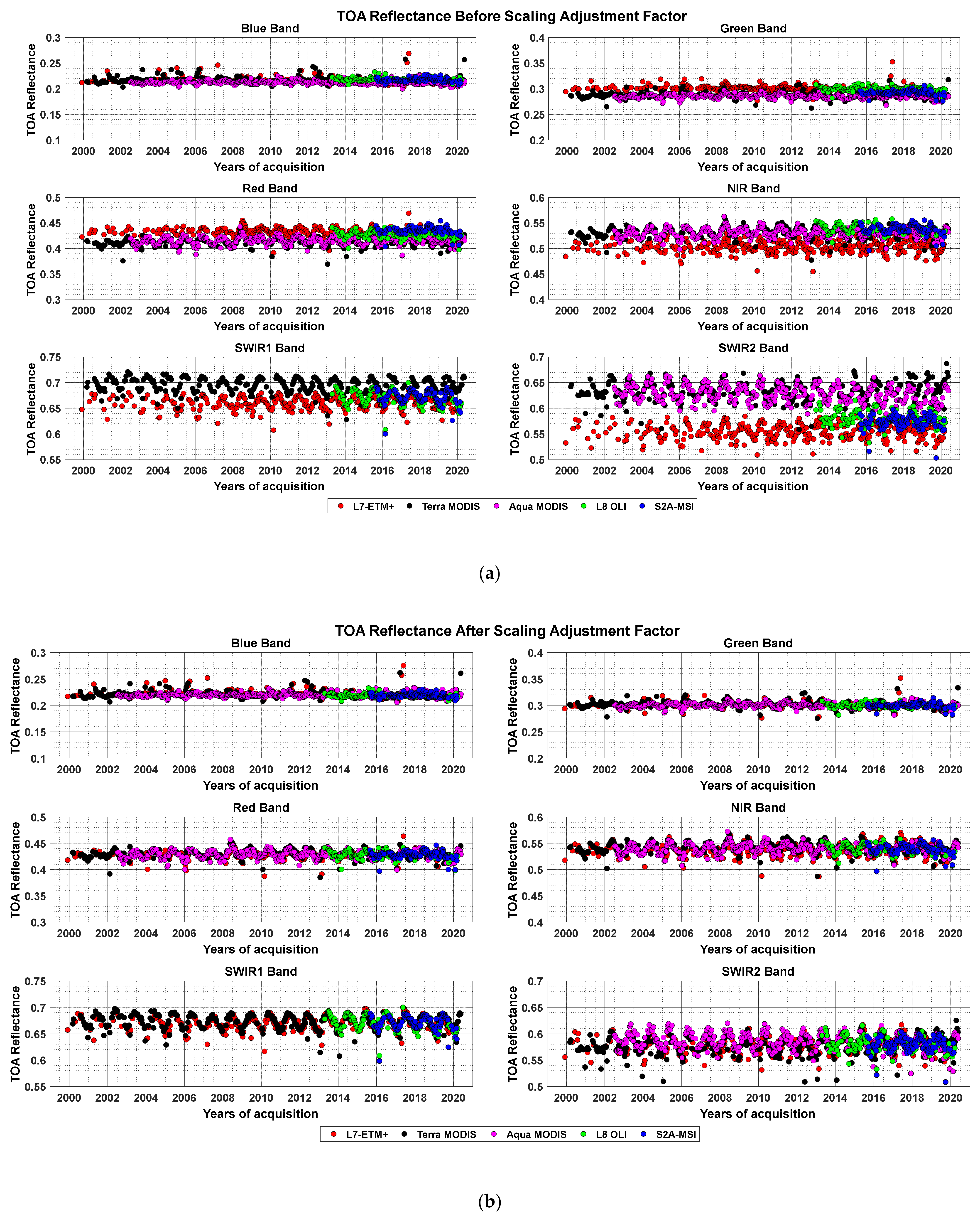
Figure 3.
Temporal trend of before (a) and after (b) scaling adjusted TOA reflectance over Sudan 1 site for the combined dataset (ETM+, Terra MODIS, Aqua MODIS, OLI, and MSI).
Figure 3.
Temporal trend of before (a) and after (b) scaling adjusted TOA reflectance over Sudan 1 site for the combined dataset (ETM+, Terra MODIS, Aqua MODIS, OLI, and MSI).
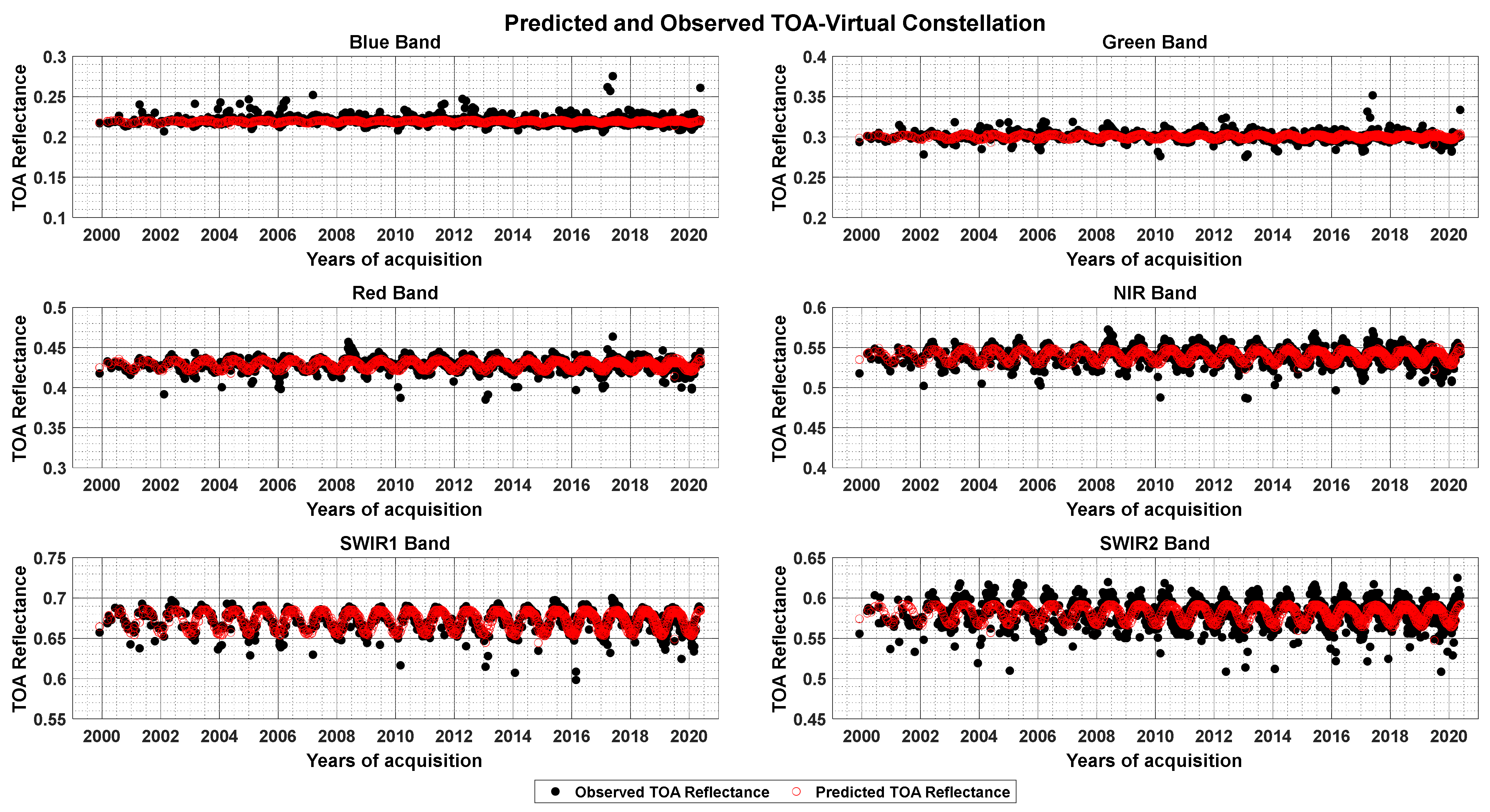
Figure 4.
In red, the TOA reflectance predicted by the BRDF model; and in black, the observed TOA reflectance data of virtual constellation over Sudan 1 for blue, green, red, NIR, SWIR 1, and SWIR 2 bands.
Figure 4.
In red, the TOA reflectance predicted by the BRDF model; and in black, the observed TOA reflectance data of virtual constellation over Sudan 1 for blue, green, red, NIR, SWIR 1, and SWIR 2 bands.
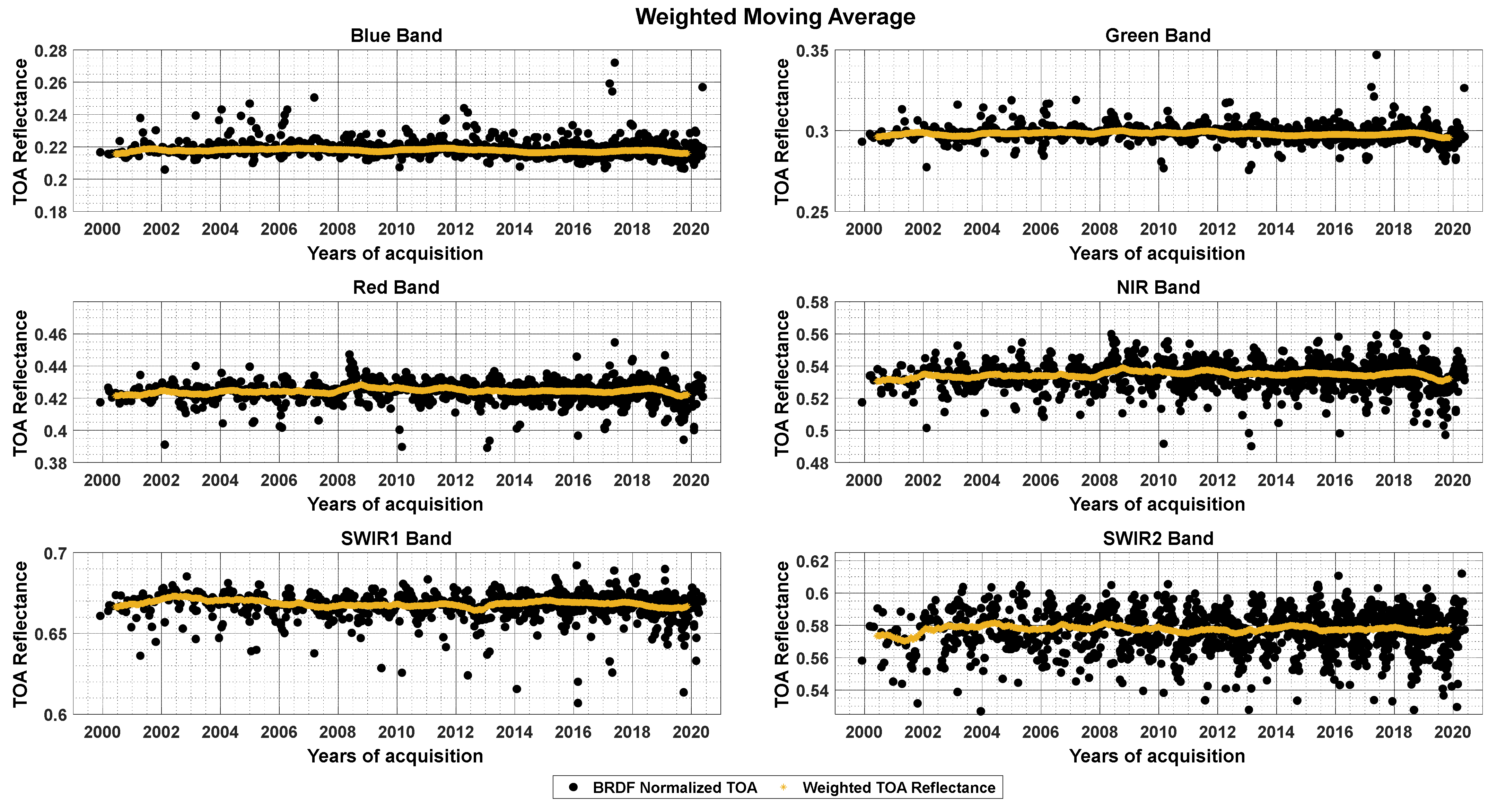
Figure 5.
Weighted moving averaged TOA reflectance data of the virtual constellation over Sudan 1 for blue, green, red, NIR, SWIR 1, and SWIR 2 bands.
Figure 5.
Weighted moving averaged TOA reflectance data of the virtual constellation over Sudan 1 for blue, green, red, NIR, SWIR 1, and SWIR 2 bands.
Figure 6.
Abrupt change in TOA reflectance data of virtual constellation over Sudan 1 for blue, green, red, NIR, SWIR 1, and SWIR 2 bands.
Figure 6.
Abrupt change in TOA reflectance data of virtual constellation over Sudan 1 for blue, green, red, NIR, SWIR 1, and SWIR 2 bands.
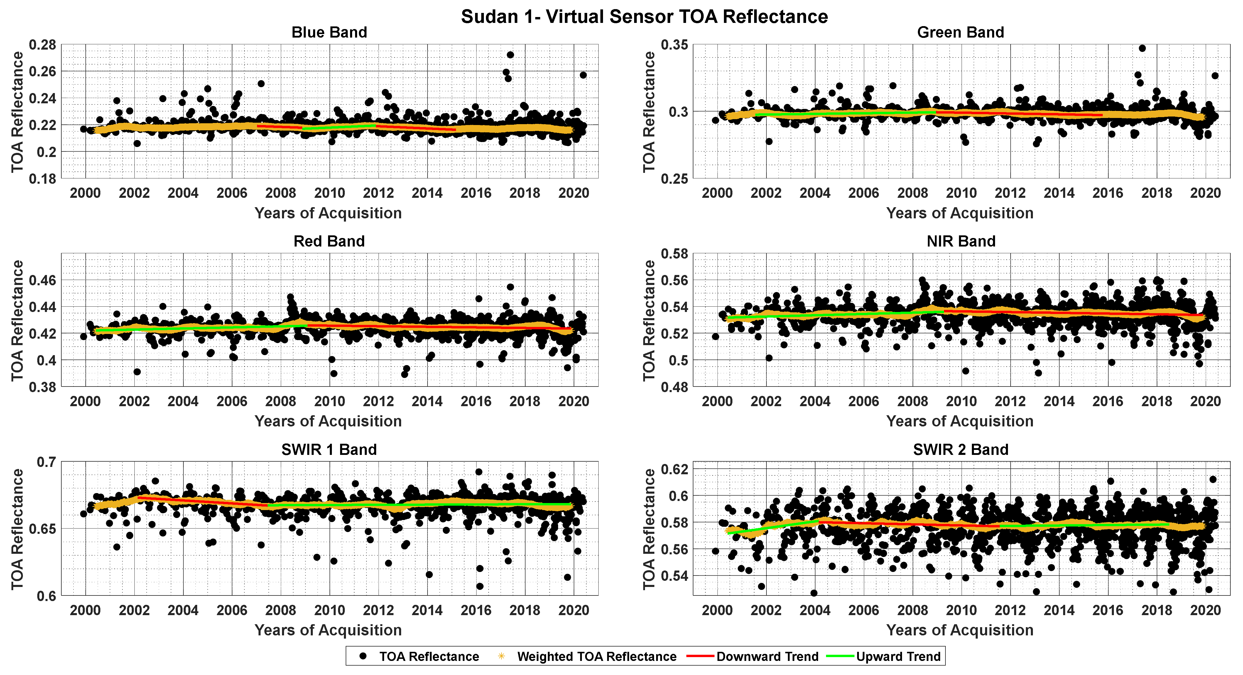
Figure 7.
TOA reflectance data of virtual constellation over Sudan 1 for blue, green, red, NIR, SWIR 1, and SWIR 2 bands with fitted trend line before and after turning points.
Figure 7.
TOA reflectance data of virtual constellation over Sudan 1 for blue, green, red, NIR, SWIR 1, and SWIR 2 bands with fitted trend line before and after turning points.
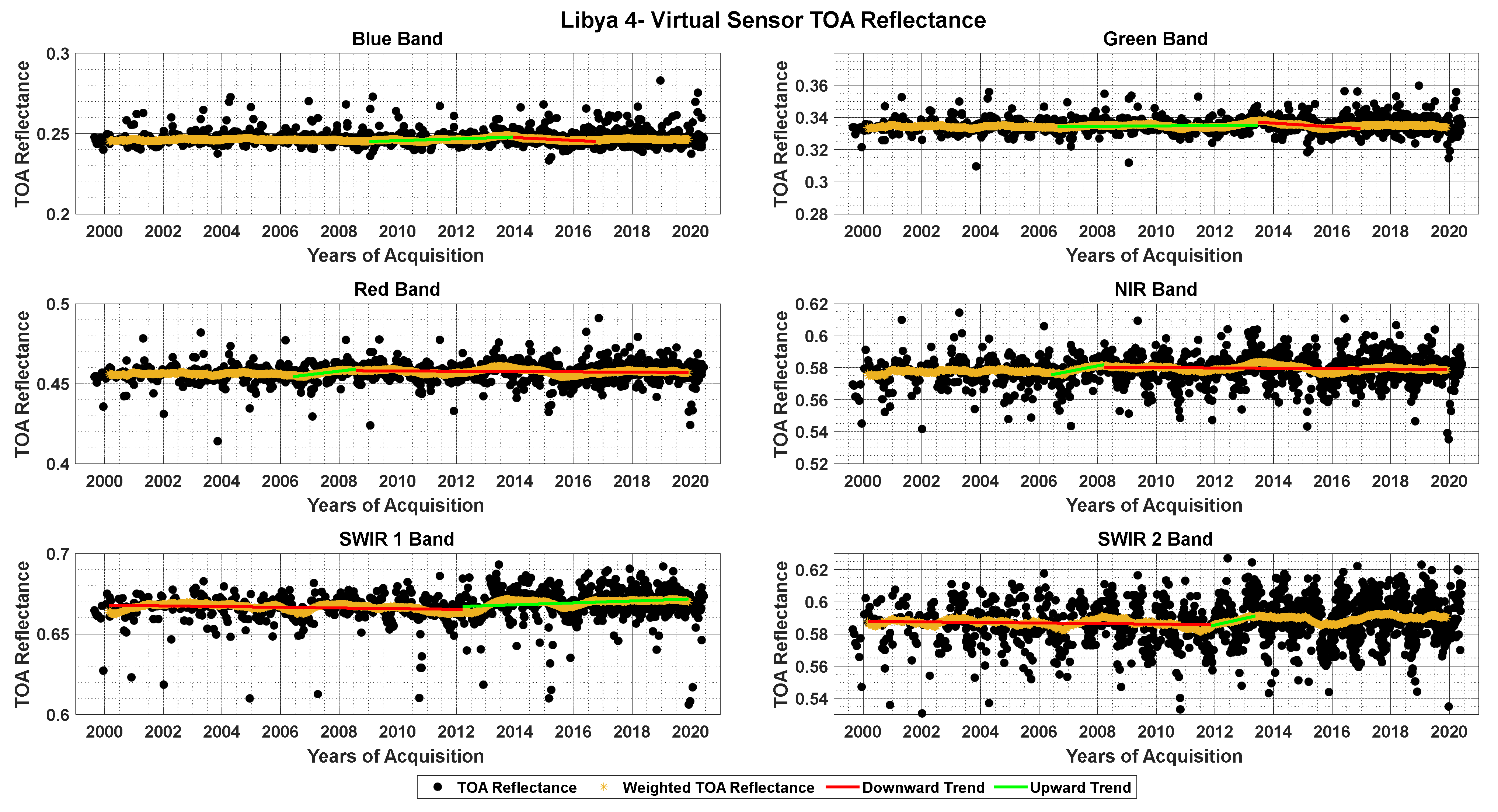
Figure 8.
TOA reflectance data of virtual constellation over Libya 4 for blue, green, red, NIR, SWIR 1, and SWIR 2 band with fitted trend lines before and after turning points.
Figure 8.
TOA reflectance data of virtual constellation over Libya 4 for blue, green, red, NIR, SWIR 1, and SWIR 2 band with fitted trend lines before and after turning points.
Figure 9.
TOA reflectance data of the virtual constellation over Egypt 1 for blue, green, red, NIR, SWIR 1, and SWIR 2 bands with fitted trend lines before and after turning points.
Figure 9.
TOA reflectance data of the virtual constellation over Egypt 1 for blue, green, red, NIR, SWIR 1, and SWIR 2 bands with fitted trend lines before and after turning points.
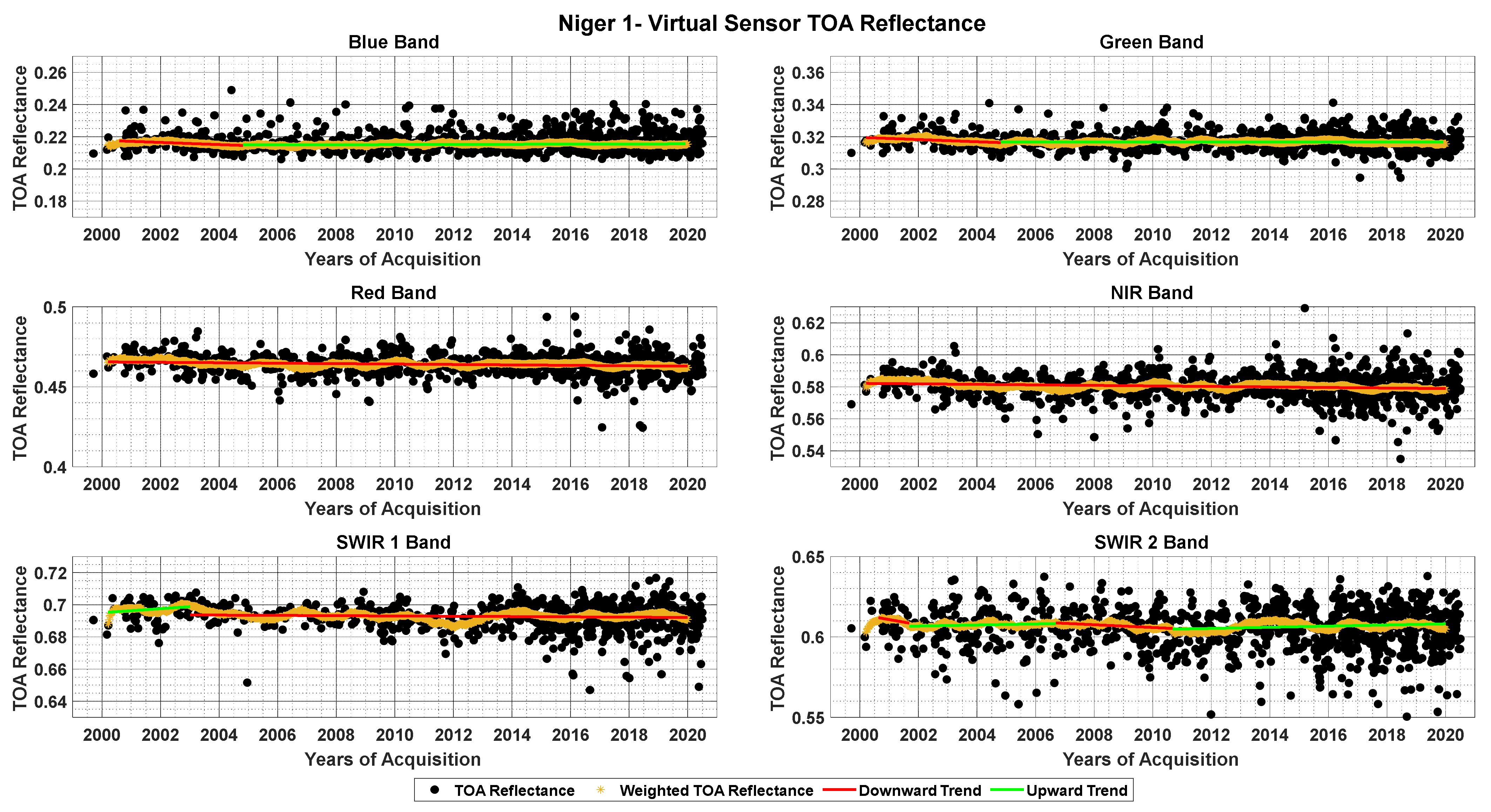
Figure 10.
TOA reflectance data of the virtual constellation over Niger 1 for blue, green, red, NIR, SWIR 1, and SWIR 2 bands with fitted trend lines before and after turning points.
Figure 10.
TOA reflectance data of the virtual constellation over Niger 1 for blue, green, red, NIR, SWIR 1, and SWIR 2 bands with fitted trend lines before and after turning points.
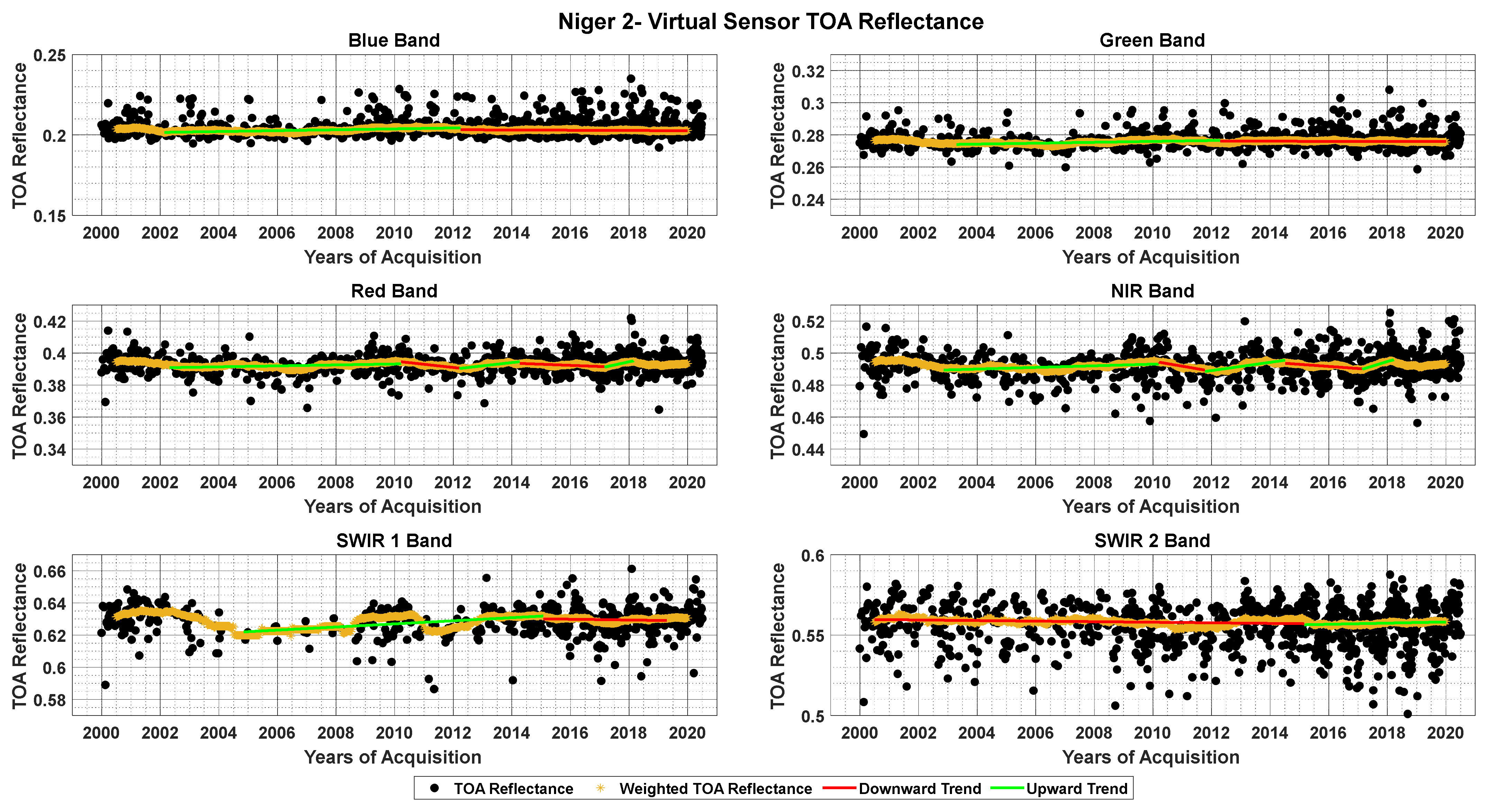
Figure 11.
TOA reflectance data of the virtual constellation over Niger 2 for blue, green, red, NIR, SWIR 1, and SWIR 2 bands with fitted trend lines before and after turning points.
Figure 11.
TOA reflectance data of the virtual constellation over Niger 2 for blue, green, red, NIR, SWIR 1, and SWIR 2 bands with fitted trend lines before and after turning points.
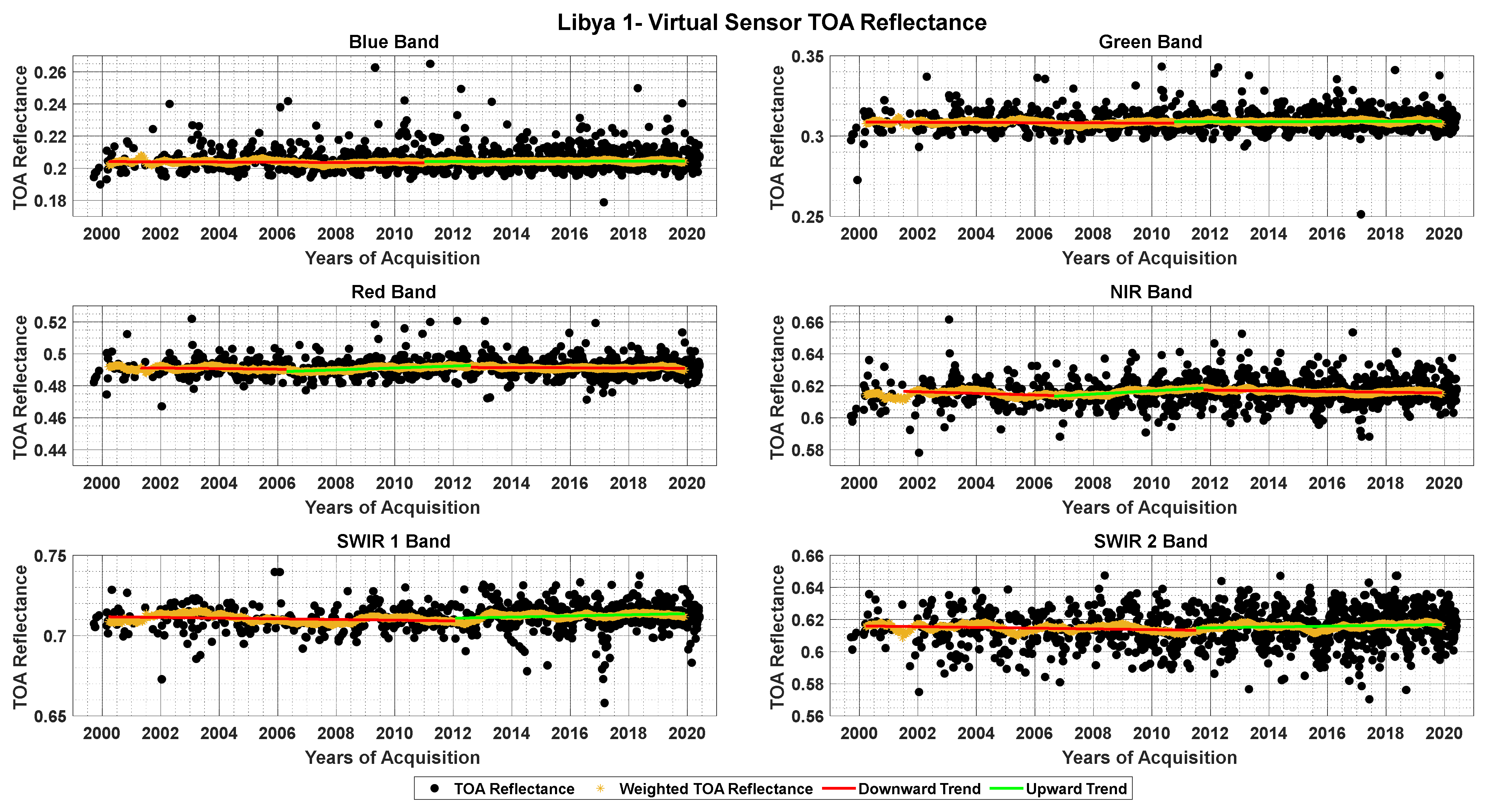
Figure 12.
TOA reflectance data of the virtual constellation over Libya 1 for blue, green, red, NIR, SWIR 1, and SWIR 2 bands with fitted trend lines before and after turning points.
Figure 12.
TOA reflectance data of the virtual constellation over Libya 1 for blue, green, red, NIR, SWIR 1, and SWIR 2 bands with fitted trend lines before and after turning points.
Table 1.
Spectral bands of satellite sensors.
Table 1.
Spectral bands of satellite sensors.
| Bandwidth (nm) |
|---|
| Sensor/Satellite | Blue | Green | Red | NIR | SWIR 1 | SWIR 2 |
|---|
| OLI/Landsat-8 | 452–12 | 533–590 | 636–673 | 851–879 | 1567–1651 | 2107–2294 |
| ETM+/Landsat-7 | 441–514 | 519–611 | 631–692 | 772–898 | 1547–1748 | 2064–2346 |
| MSI/Sentinel-2A | 470–524 | 504–602 | 649–680 | 855–875 | 1569–1658 | 2113–2286 |
| MODIS/TERRA | 459–479 | 545–565 | 620–670 | 841–876 | 1628–1652 | 2105–2155 |
| MODIS/AQUA | 459–479 | 545–565 | 620–670 | 841–876 | 1628–1652 | 2105–2155 |
Table 2.
Location of study areas, including the WRS-2 Path/Row, UTM/WGS84 Tiles, and ROI coordinates.
Table 2.
Location of study areas, including the WRS-2 Path/Row, UTM/WGS84 Tiles, and ROI coordinates.
| PICS | WRS-2 Path/Row | MSI Tile | Minimum
Latitude | Maximum Latitude | Minimum
Longitude | Maximum Longitude |
|---|
| Libya 4 | 181/40 | 34RGS | 28.38 | 28.81 | 23.09 | 23.86 |
| Niger 1 | 189/46 | 32QNH | 20.28 | 20.53 | 9.19 | 9.52 |
| Sudan1 | 177/45 | 35QND | 21.40 | 21.75 | 27.81 | 27.59 |
| Niger 2 | 188/45 | 32QPJ | 21.25 | 21.47 | 10.38 | 10.71 |
| Egypt 1 | 179/41 | 35RMK | 26.91 | 27.13 | 26.31 | 26.62 |
| Libya 1 | 187/43 | 33RUH | 24.55 | 24.86 | 13.32 | 13.66 |
Table 3.
Reference angles for PICS.
Table 3.
Reference angles for PICS.
| SZA | SAA | VZA | VAA |
|---|
| 38° | 144° | 3° | 103° |
Table 4.
Sensor calibration uncertainty for five different sensors [
21,
22,
25,
27,
28].
Table 4.
Sensor calibration uncertainty for five different sensors [
21,
22,
25,
27,
28].
| Sensors | Reflectance Product Uncertainty |
|---|
| L7- ETM+ | 5% |
| L8-OLI | 2% |
| Sentinel 2A | 2.5% |
| Terra MODIS | 2% |
| Aqua MODIS | 2% |
Table 5.
BRDF model error (residual error) in percentage for all PICS sites in matching spectral bands.
Table 5.
BRDF model error (residual error) in percentage for all PICS sites in matching spectral bands.
| Bands | Sudan 1 | Libya 4 | Egypt 1 | Niger 1 | Libya 1 | Niger 2 |
|---|
| Blue | 0.304% | 0.259% | 0.107% | 0.385% | 0.398% | 0.611% |
| Green | 0.032% | 0.059% | −0.017% | 0.083% | 0.128% | 0.281% |
| Red | −0.113% | −0.043% | −0.056% | −0.045% | 0.013% | −0.007% |
| NIR | −0.116% | −0.083% | −0.055% | −0.055% | −0.014% | −0.056% |
| SWIR 1 | −0.194% | −0.170% | −0.055% | −0.167% | −0.145% | −0.120% |
| SWIR 2 | −0.231% | −0.351% | −0.092% | −0.270% | −0.162% | −0.261% |
Table 6.
Total average estimated uncertainty for all PICS sites in matching spectral bands.
Table 6.
Total average estimated uncertainty for all PICS sites in matching spectral bands.
| Bands | Libya 1 | Libya 4 | Niger 1 | Niger 2 | Sudan 1 | Egypt 1 |
|---|
| Blue | 6.21% | 4.89% | 5.43% | 5.57% | 4.52% | 4.59% |
| Green | 4.95% | 4.85% | 4.24% | 4.59% | 4.06% | 4.68% |
| Red | 4.34% | 4.87% | 4.00% | 4.25% | 4.07% | 4.63% |
| NIR | 4.47% | 5.07% | 4.06% | 4.33% | 4.07% | 4.57% |
| SWIR 1 | 5.20% | 5.54% | 4.20% | 4.63% | 4.25% | 4.63% |
| SWIR 2 | 5.58% | 6.34% | 4.95% | 5.31% | 4.95% | 4.82% |
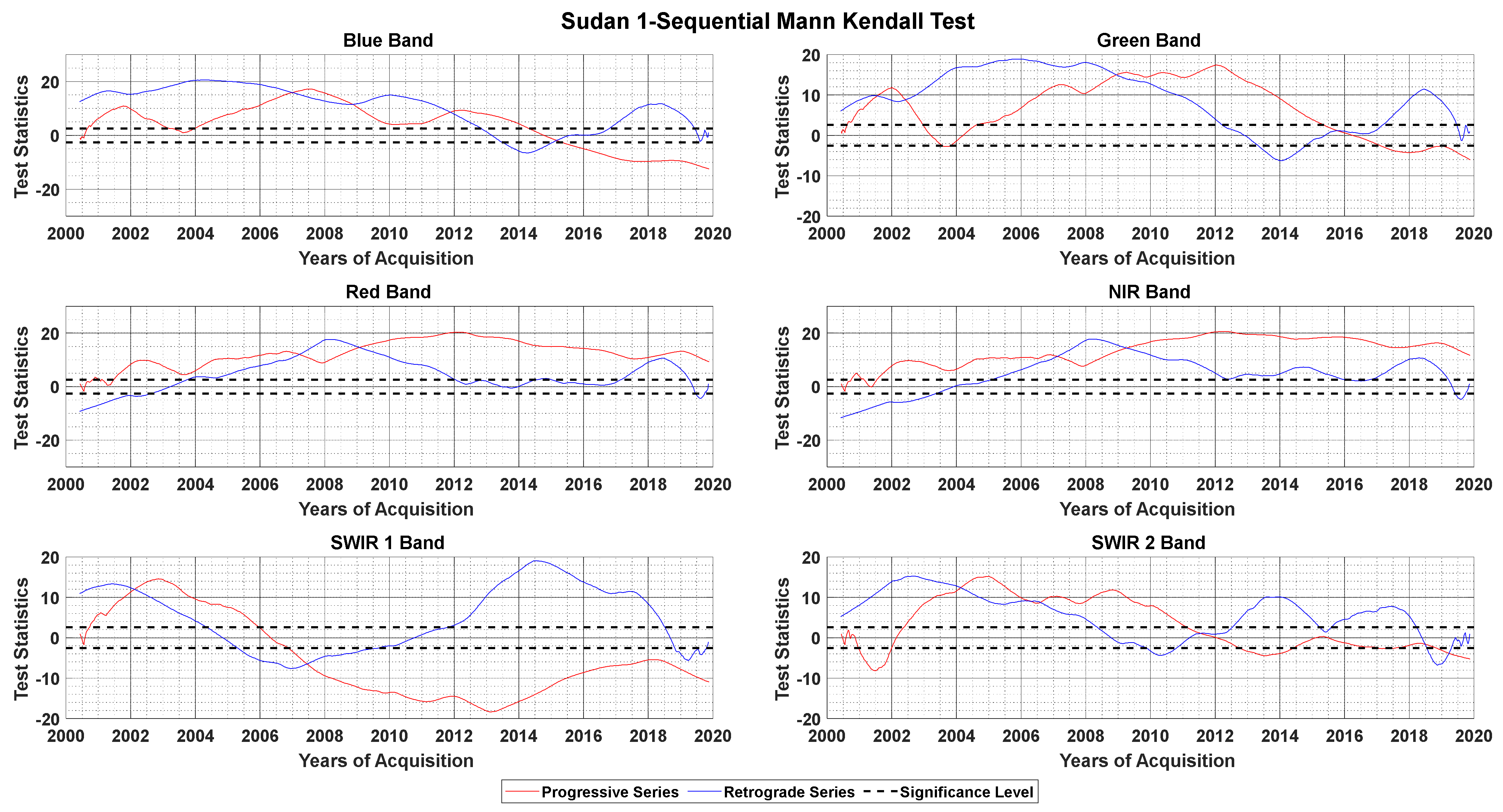
Table 7.
Change point detection by the sequential version of the Mann–Kendall test for Sudan 1.
Table 7.
Change point detection by the sequential version of the Mann–Kendall test for Sudan 1.
| Bands | Detected Change Points (Year) | Remarks |
|---|
| 2nd | 3rd | 4th | 5th |
|---|
| Blue | 2007 * | 2009 * | 2011 * | 2015 * | - | Significant |
| Green | 2001 * | 2002 * | 2009 * | 2015 | - | Significant |
| Red | 2007 * | 2009 * | - | - | - | Significant |
| NIR | 2007 * | 2009 * | - | - | - | Significant |
| SWIR 1 | 2002 * | 2007 * | - | - | - | Significant |
| SWIR 2 | 2004 * | 2007 * | 2011 | 2018 | 2019 * | Significant |
Table 8.
Mann–Kendall test results at 0.01 significance level for Sudan 1.
Table 8.
Mann–Kendall test results at 0.01 significance level for Sudan 1.
| Bands | Weighted TOA Reflectance Data | Unweighted TOA Reflectance Data |
|---|
| p-Value | Decision | p-Value | Decision |
|---|
| Blue | | Downward Trend | | Downward Trend |
| Green | | Downward Trend | | Downward Trend |
| Red | | Upward Trend | 0.258 | No Trend |
| NIR | | Upward Trend | 0.932 | No Trend |
| SWIR 1 | | Downward Trend | 0.036 | No Trend |
| SWIR 2 | | Downward Trend | 0.594 | No Trend |
Table 9.
Change point detection by sequential version of the Mann–Kendall test for Libya 4.
Table 9.
Change point detection by sequential version of the Mann–Kendall test for Libya 4.
| Bands | Detected Change Points (Year) | Remarks |
|---|
| 2nd | 3rd | 4th | 5th |
|---|
| Blue | 2009 * | 2013 * | 2016 | 2018 * | - | Significant |
| Green | 2006 | 2008 * | 2011 * | 2013 * | 2017 * | Significant |
| Red | 2006 | 2008 * | - | - | - | Significant |
| NIR | 2006 | 2008 * | - | - | - | Significant |
| SWIR 1 | 2012 * | 2013 * | - | - | - | Significant |
| SWIR 2 | 2011 * | 2013 * | 2017 * | - | - | Significant |
Table 10.
Change point detection by the sequential version of the Mann–Kendall test for Egypt 1.
Table 10.
Change point detection by the sequential version of the Mann–Kendall test for Egypt 1.
| Bands | Detected Change Points (Year) | Remarks |
|---|
| 2nd | 3rd |
|---|
| Blue | 2017 * | 2019 * | - | Significant |
| Green | 2017 * | 2019 * | - | Significant |
| Red | 2006 * | 2017 * | 2019 | Significant |
| NIR | 2006 * | 2017 * | 2019 | Significant |
| SWIR 1 | 2016 * | 2018 | - | Significant |
| SWIR 2 | 2016 * | 2018 | - | Significant |
Table 11.
Change point detection by sequential versions of the Mann–Kendall test for Niger 1.
Table 11.
Change point detection by sequential versions of the Mann–Kendall test for Niger 1.
| Bands | Detected Change Points (Year) | Remarks |
|---|
| | | | |
|---|
| Blue | 2000 | 2004 * | 2016 | 2018 | 2019 | Significant |
| Green | 2001 | 2003 * | - | - | - | Significant |
| Red | - | - | - | - | - | |
| NIR | - | - | - | - | - | |
| SWIR 1 | 2003 * | 2004 | - | - | - | Significant |
| SWIR 2 | 2000 | 2001 * | 2006 * | 2010 * | - | Significant |
Table 12.
Change point detection by sequential version of the Mann–Kendall test for Niger 2.
Table 12.
Change point detection by sequential version of the Mann–Kendall test for Niger 2.
| Bands | Detected Change Points (Year) | Remarks |
|---|
| | 3rd | 4th | 5th | 6th |
|---|
| Blue | 2002 * | 2012 * | 2013 | 2016 | 2017 | - | Significant |
| Green | 2003 * | 2004 | 2010 | 2012 * | 2015 | 2017 | Significant |
| Red | 2002 * | 2010 * | 2012 * | 2014 * | 2017 * | 2018 * | Significant |
| NIR | 2002 * | 2010 * | 2011 * | 2014 * | 2017 * | 2018 * | Significant |
| SWIR 1 | 2004 * | 2015 * | - | - | - | - | Significant |
| SWIR 2 | 2015 * | 2016 | - | - | - | - | Significant |
Table 13.
Change point detection by sequential versions of the Mann–Kendall tests for Libya 1.
Table 13.
Change point detection by sequential versions of the Mann–Kendall tests for Libya 1.
| Bands | Detected Change Points (Year) | Remarks |
|---|
| 2nd | 3rd | 4th | 5th |
|---|
| Blue | 2011 * | - | - | - | - | Significant |
| Green | 2008 * | 2011 * | - | - | - | Significant |
| Red | 2001 * | 2006 * | 2012 * | 2018 | 2019 * | Significant |
| NIR | 2001 * | 2006 * | 2012 * | - | - | Significant |
| SWIR 1 | 2012 * | 2014 * | 2017 * | - | - | Significant |
| SWIR 2 | 2011 * | 2012 * | 2019 * | - | - | Significant |
Table 14.
Summary of Mann–Kendall test results for overall time series for Libya 1, Egypt 1, Niger 1, Niger 2 and Libya 1.
Table 14.
Summary of Mann–Kendall test results for overall time series for Libya 1, Egypt 1, Niger 1, Niger 2 and Libya 1.
| Bands | p-Value | Decision |
|---|
| Libya 4 |
| Blue | | Upward Trend |
| Green | | Upward Trend |
| Red | | Upward Trend |
| NIR | | Upward Trend |
| SWIR 1 | | Upward Trend |
| SWIR 2 | | Upward Trend |
| Egypt 1 |
| Blue | | Upward Trend |
| Green | | Upward Trend |
| Red | | Upward Trend |
| NIR | | Upward Trend |
| SWIR 1 | | Upward Trend |
| SWIR 2 | | Upward Trend |
| Niger 1 |
| Blue | 0.002 | No Trend |
| Green | | Downward Trend |
| Red | | Downward Trend |
| NIR | | Downward Trend |
| SWIR 1 | | Downward Trend |
| SWIR 2 | | Downward Trend |
| Niger 2 |
| Blue | 0.033 | No Trend |
| Green | | Upward Trend |
| Red | 0.031 | No Trend |
| NIR | 0.041 | No Trend |
| SWIR 1 | 0.532 | No Trend |
| SWIR 2 | | Downward Trend |
| Libya 1 |
| Blue | | Upward Trend |
| Green | | Upward Trend |
| Red | | Upward Trend |
| NIR | | Upward Trend |
| SWIR 1 | | Upward Trend |
| SWIR 2 | | Upward Trend |
Table 15.
Summary of long-term TOA reflectance change per year (in %) for all PICS.
Table 15.
Summary of long-term TOA reflectance change per year (in %) for all PICS.
| Bands | Sudan 1 | Libya 4 | Egypt 1 | Niger 1 | Libya 1 | Niger 2 |
|---|
| Blue | −0.028% | 0.008% | 0.042% | - | 0.019% | - |
| Green | −0.011% | 0.013% | 0.026% | −0.022% | 0.015% | 0.010% |
| Red | 0.016% | 0.019% | 0.019% | −0.028% | 0.006% | - |
| NIR | 0.019% | 0.019% | 0.017% | −0.029% | 0.015% | - |
| SWIR 1 | −0.018% | 0.002% | 0.015% | −0.028% | 0.019% | - |
| SWIR 2 | −0.009% | 0.039% | 0.025% | −0.012% | 0.011% | −0.215% |


