
On the Optimal Tilt Angle and Orientation of an On-Site Solar Photovoltaic Energy Generation System for Sabah’s Rural Electrification

 ,
, 
 and
and
Abstract
1. Introduction
1.1. Research Background
1.2. Literature Review
Solar Models
1.3. Study Contribution
- To find the optimum tilt angle, , and the orientation of the solar PV modules at EPLISSI that could provide the maximum monthly insolation, H, throughout the year by applying the Liu and Jordan isotropic diffuse sky radiation model; and to identify the suitable tilt angle and orientation by using the Liu and Jordan empirical model with the variation of conditions listed as follows:
- The collector’s orientation is kept in facing due south position throughout the year.
- Both the tilt angle and orientation could be adjusted throughout the year.
- Both tilt angle and orientation (facing due south) are fixed.
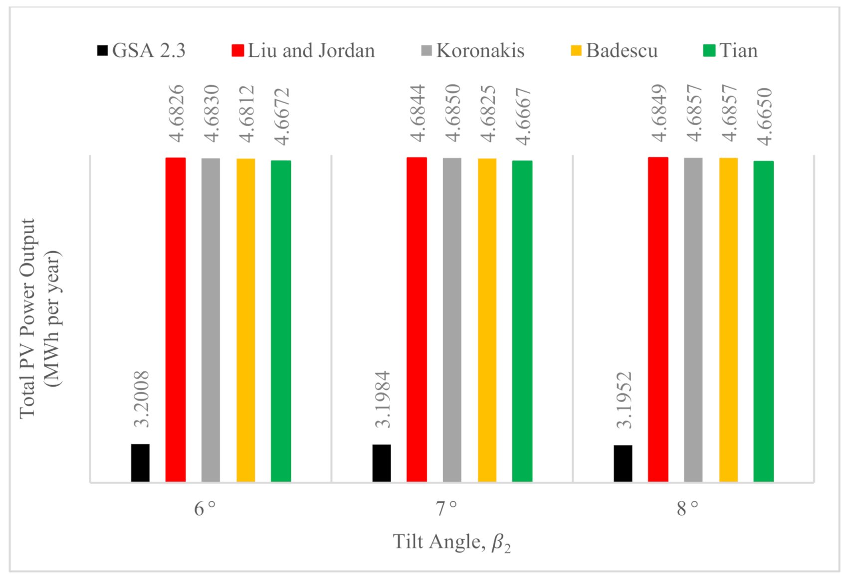
- To find the optimum tilt angle, , at EPLISSI by applying four isotropic models known as the Liu and Jordan, Koronakis, Badescu, and Tian models and identifying the highest solar irradiation value. The orientation is fixed facing due south. The results of total PV power output found through each of the models will be compared to results simulated using Global Solar Atlas version 2.3 or GSA 2.3 to determine the most preferred model to estimate the total solar irradiance in EPLISSI.
2. Methodology
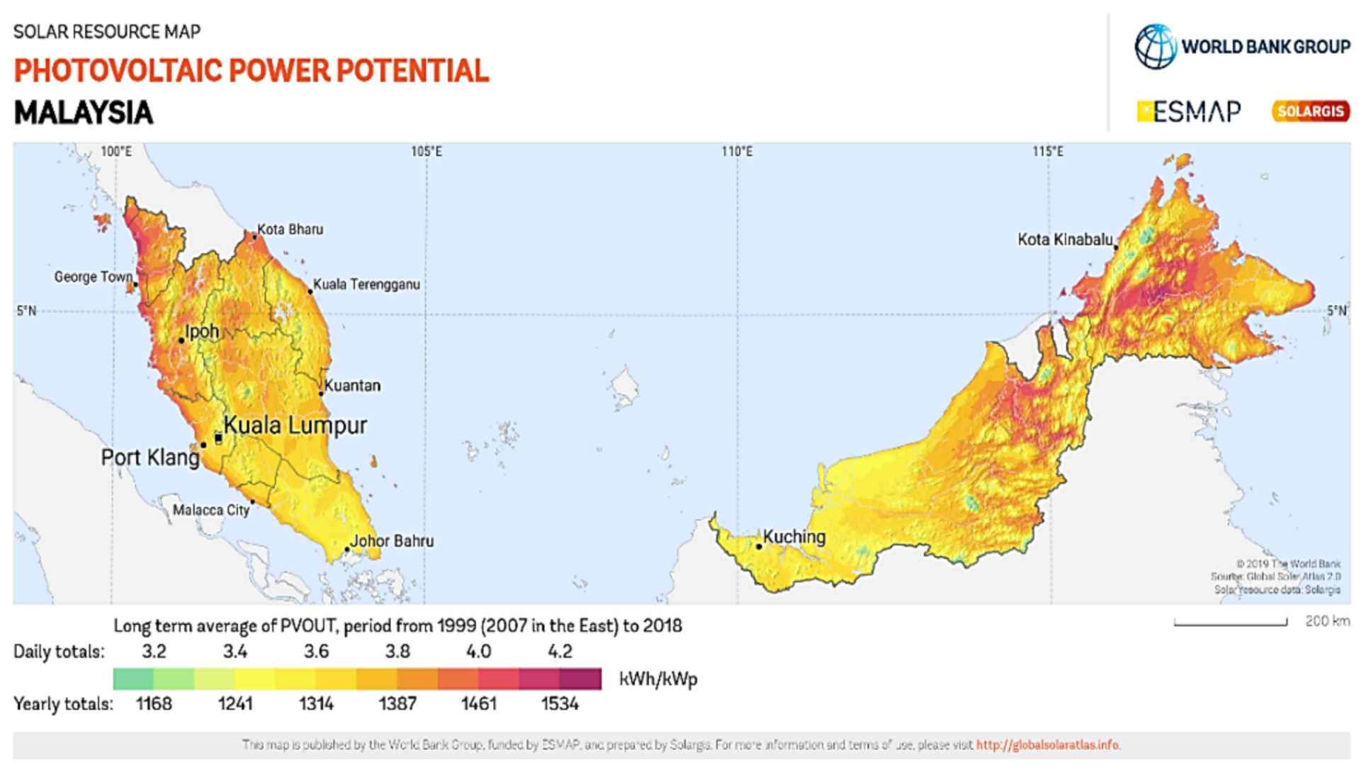
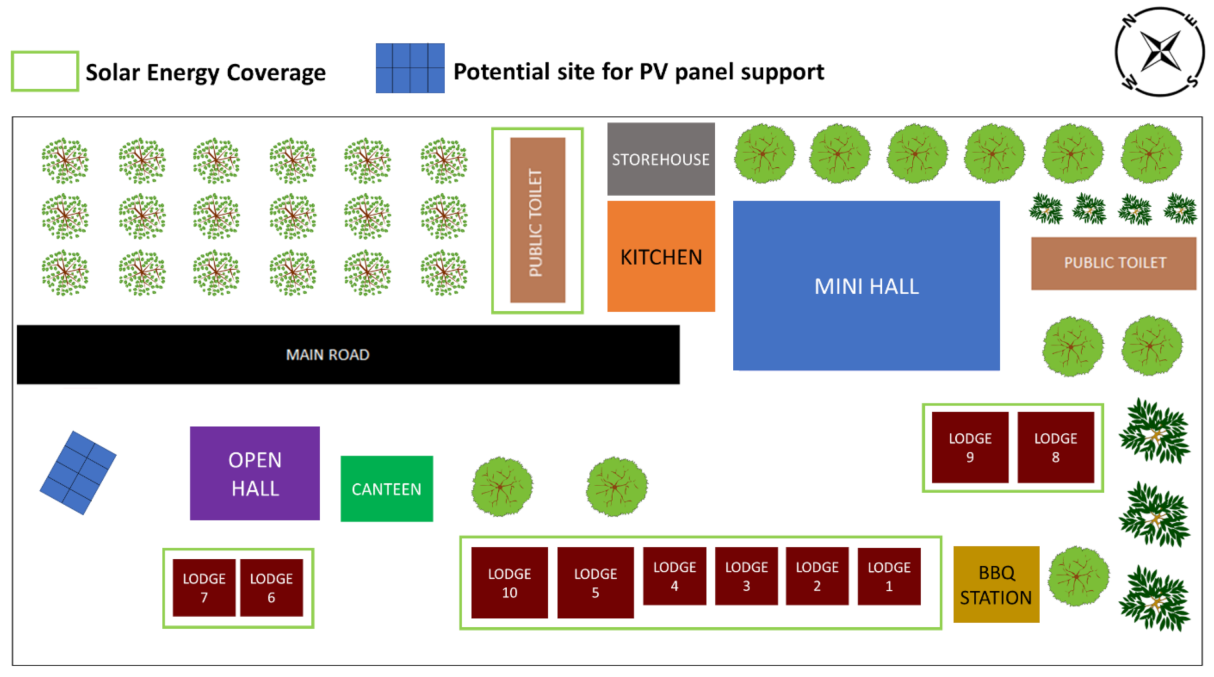
2.1. Study Location
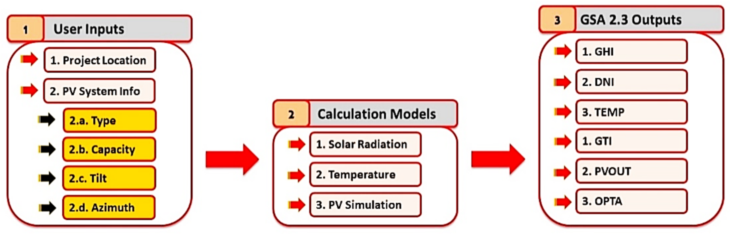
2.2. Global Solar Atlas PV Data Simulator
- The clear-sky irradiance (the irradiance touching the ground with the assumption of lack of clouds) is computed using the clear-sky model.
- The satellite data (data from several geostationary satellites) quantifies the attenuation effect of clouds through cloud index computation. The clear-sky irradiance is combined with the cloud index to retrieve all-sky irradiance. This process results in direct normal irradiance (DNI) and global horizontal irradiance (GHI).
- The DNI and GHI are utilised for computing diffuse and global tilted irradiance (irradiance in plane of the array, on tilted or tracking surfaces) and/or irradiance rectified for shading effects from surrounding terrain or nearby objects.
- Inadequate ventilation of PV modules mounted on roofs is considered; hence the output will be reduced due to the higher temperature of modules.
- The roof systems are usually installed at a sub-optimal inclination, which means that the access for cleaning is limited, thus increased collection of dust and soiling on modules is likely to happen.
- Cabling paths are short, directly linked into inverters (no combiner boxes), and generated AC power is evacuated into the grid directly from the inverter without a transformer.
- The availability is reduced because detailed monitoring systems are rarely utilised, and repair service in case of a failure may last several days.
2.3. The Application of the Liu and Jordan Isotropic Diffuse Sky Radiation Model to Estimate the Optimal Tilt Angle and Orientation of the Solar Photovoltaic Module
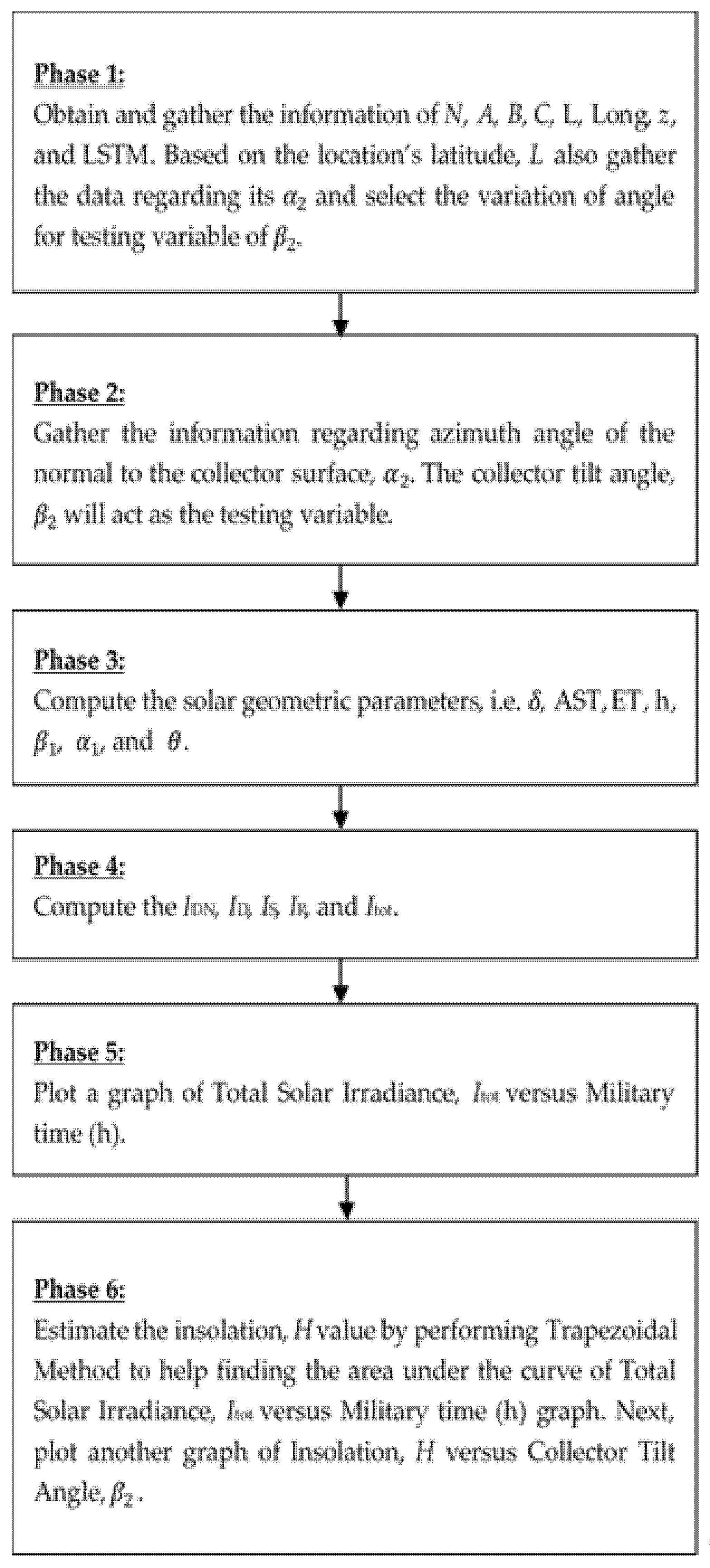
- Phase 1
- Phase 2
- Phase 3
- Phase 4
- Phase 5
- Phase 6
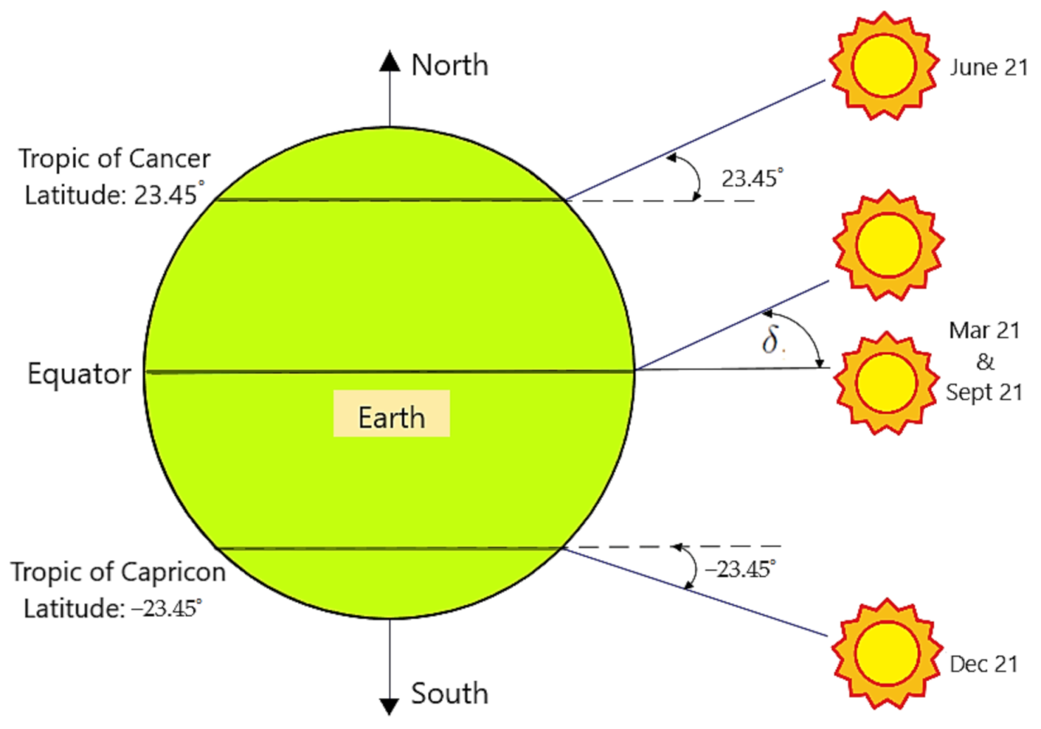
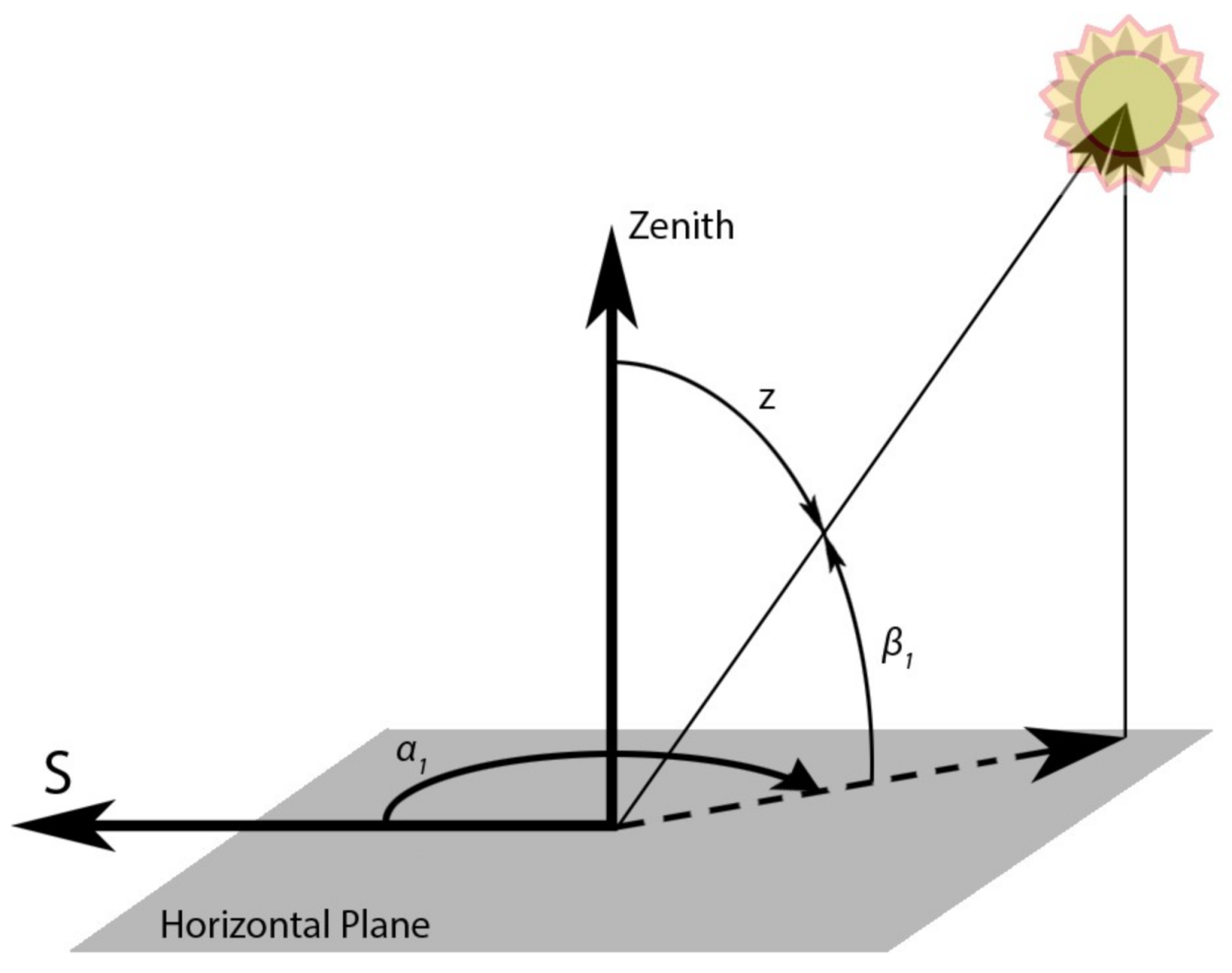
- Time and solar angles: The declination angle, δ, is the sun’s angular displacement to the earth’s equator (refer to Figure 5). For the northern hemisphere, δ is given in degrees by Equation (1) below [34,55,56,57]:where N is the day number of the year. The 23.45 is known as the mean oblique ecliptic, and its sign is positive for the northern hemisphere and negative for the southern hemisphere. The δ varies between 23.5 (northern summer solstice) to −23.5 (southern summer solstice). The Earth’s surface is divided into a grid consisting of lines known as latitude, L, and longitude, Long. For Long, the origin 0 is known as the prime meridian (the north-south line that passes through Greenwich, England), whereas for L, the origin 0 is the equator.To traverse one degree of Long, it would take up to four minutes by recognising that there are 24 h/day, 60 min/hour, and 1440 min/day. The apparent solar time, AST, or local solar time for eastern longitudes, is given in minutes by Equation (2) below [56,57]:LST stands for local standard time (given in minutes), LSTM is local standard time meridian, Long is longitude, and ET is the equation of time. ET is a measure of the extent by which solar time runs faster or slower than an everyday running clock running at a uniform rate. It is given in minutes by Equation (3) below [56,57]:where,The hour angle, h, is the sun’s angular position to the west or east of the local meridian. Before solar noon (solar noon means h = 0), the sign of h is negative (morning), whereas its sign is positive after solar noon (afternoon), and it is related to AST given in degrees by the Equation (5) below [56,57]:Figure 6 shows a fixed PV module lying flat or horizontally on the earth’s surface. The solar altitude angle, is the sun’s apparent angular position (if a person is standing in such a way that the person is directly facing the sun).After calculation, if is showing negative values, it means that the earth shades the sunlight; hence, there is no solar radiation at the given time, and the total solar radiation, is equal to zero. It is given in radian by Equation (6) below [55,56,57]:where L stands for latitude (sign is positive in either north or south hemisphere), is declination angle, and h is hour angle. On the other hand, the solar azimuth angle, , is the angular position of the sun viewed from the north-south line, which is given in radian by Equation (7) below [56,57]:Shown with a sign, the solar azimuth angle will be negative in the morning, and after solar noon, it will be positive. This is to follow the clockwise direction, and the sign of matches that of the hour angle, h.
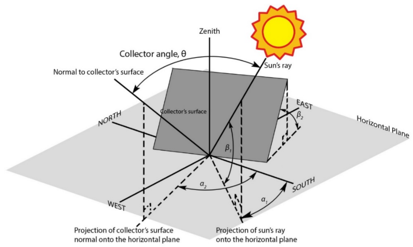
- Collector angles: In this study, the term collector is specified on the solar PV system, that is, the solar PV module. The collector tilt angle, , and orientation define the position of a solar PV module. Figure 7 illustrates a fixed PV module facing south-west ( and 0).As seen in the figure above, measures the angle of the collector surface from the ground. The collector angle, is the angle between the sun and the normal to the collector surface. The collector angle is calculated in radian as shown by Equation (8) below [56,57]:where is the solar altitude angle, is the solar azimuth angle, and is the azimuth angle of the normal to the collector surface. After calculation, if the collector angle, , is more than 90, it means that the collector is installed in such a way that the collector shades itself.
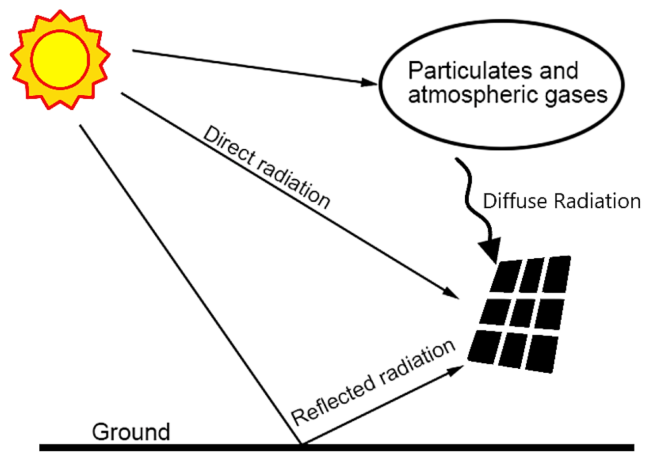
- Solar irradiance: Total solar irradiance, , is the total solar energy incident upon a surface. Figure 8 illustrates the components of solar irradiance.As seen, the direct irradiance, ID; diffuse irradiance or sky radiation, IS; and reflected irradiance, IR, are the three components of solar irradiance expressed in W/m2 [34]. The sum of these three components will be the total solar irradiance, which is given by Equation (9) below (output value would be in W/m2) [56,57]:The direct irradiance, ID, is calculated by Equation (10), where the direct normal irradiance, IDN (W/m2), is found by using Equations (11) and (12); in addition, it is used to find the atmospheric pressure relative to a standard atmosphere, (unitless) [56,57,58]:where is the collector angle, A is the apparent solar irradiation or apparent extra-terrestrial solar intensity, B is the atmospheric extinction coefficient, and z is the elevation (in kilometres above the sea level). The diffuse irradiance, , is given by the following Equation (13) [56,57,59]:where,where is the Liu and Jordan’s [59] ratio of the average daily diffuse radiation on a tilted surface to that on a horizontal surface, is the module or collector tilt angle, and C is the ratio of diffuse radiation on a horizontal surface to direct normal irradiation. The reflected irradiance, , is denoted in Equation (15) [56,57,58], where is the foreground reflectivity (Table 3 shows the typically used values of ). Note that the approximate total solar irradiance, Itot, given by only applies to the clear sky condition, whereas in cases of cloudy or overcast sky, additional information is needed to reduce the quantity of irradiance accordingly.The insolation, H, also known as solar irradiation or solar radiant exposure, is the incident solar energy per unit of surface area (unit is J/m2). H is found by integrating the Itot over a specific time. Hence,where the period is usually taken for one whole day. H is also the daily total solar energy incident on a unit surface of a module or collector. Therefore, the daily total solar energy, , can be obtained if the insolation, H, is multiplied by the surface area of a collector, Acollector (m2). It is given in joules by Equation (17) below (unit is J or Wh):
- Total solar photovoltaic power output: By using the theoretical formula, the total electrical energy generated, , by using the collector or total solar photovoltaic power output can be obtained by multiplying daily total solar energy, , with the solar cell efficiency, , denoted in Equation (18) as follows (unit is J or Wh):where the typical range of solar cell efficiency, , is approximately 0.15 to 0.25 (15% to 25%), and taken to be 0.20 (mean of the given range) in this study. To compute the yearly data set, the total number of days in a year is assumed to be 365 (does not assume leap year). Table 4 shows the data of the respective month, from January to December, assumed in this study.
2.4. Isotropic Diffuse Sky Radiation Models
3. Results and Discussions
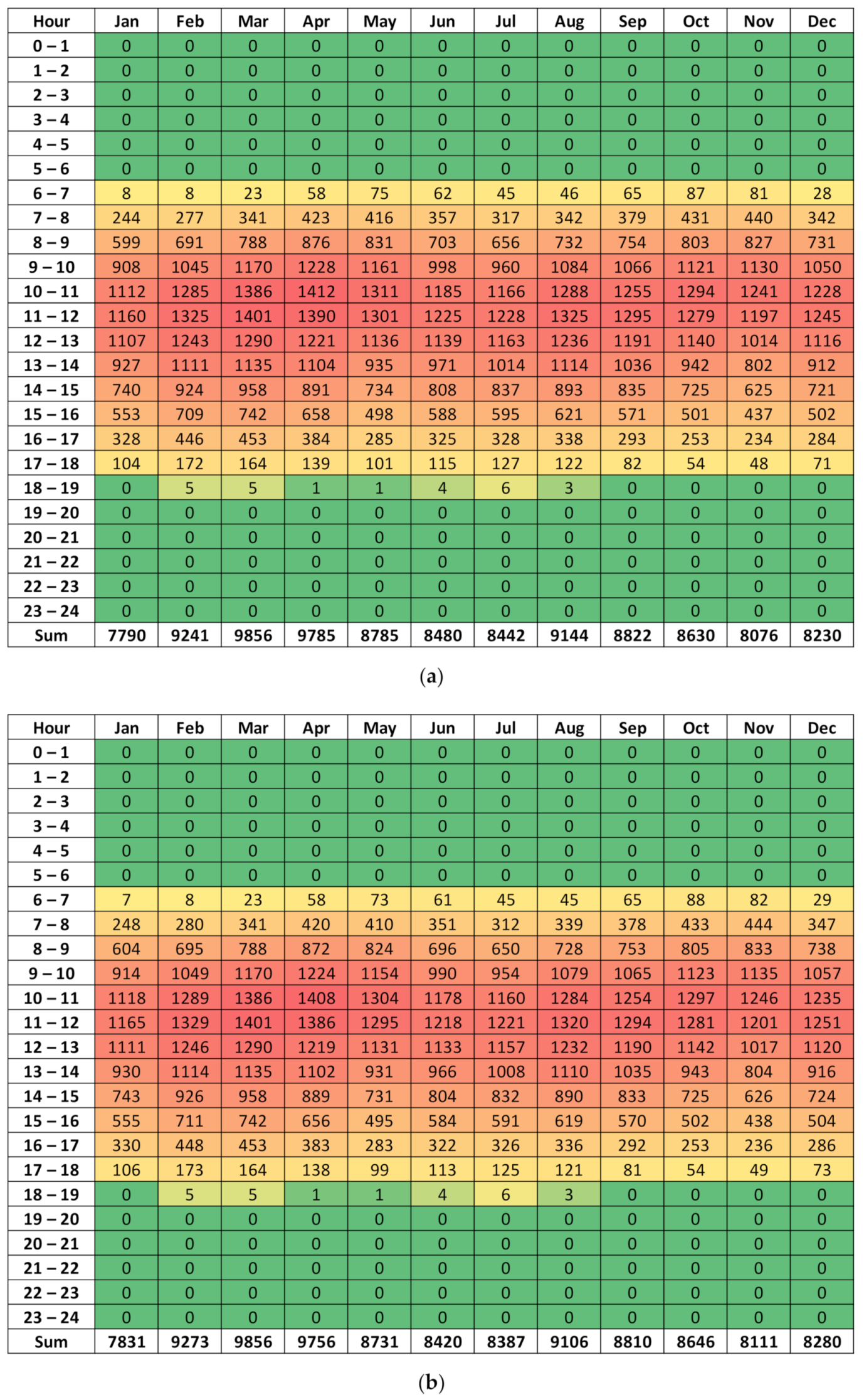
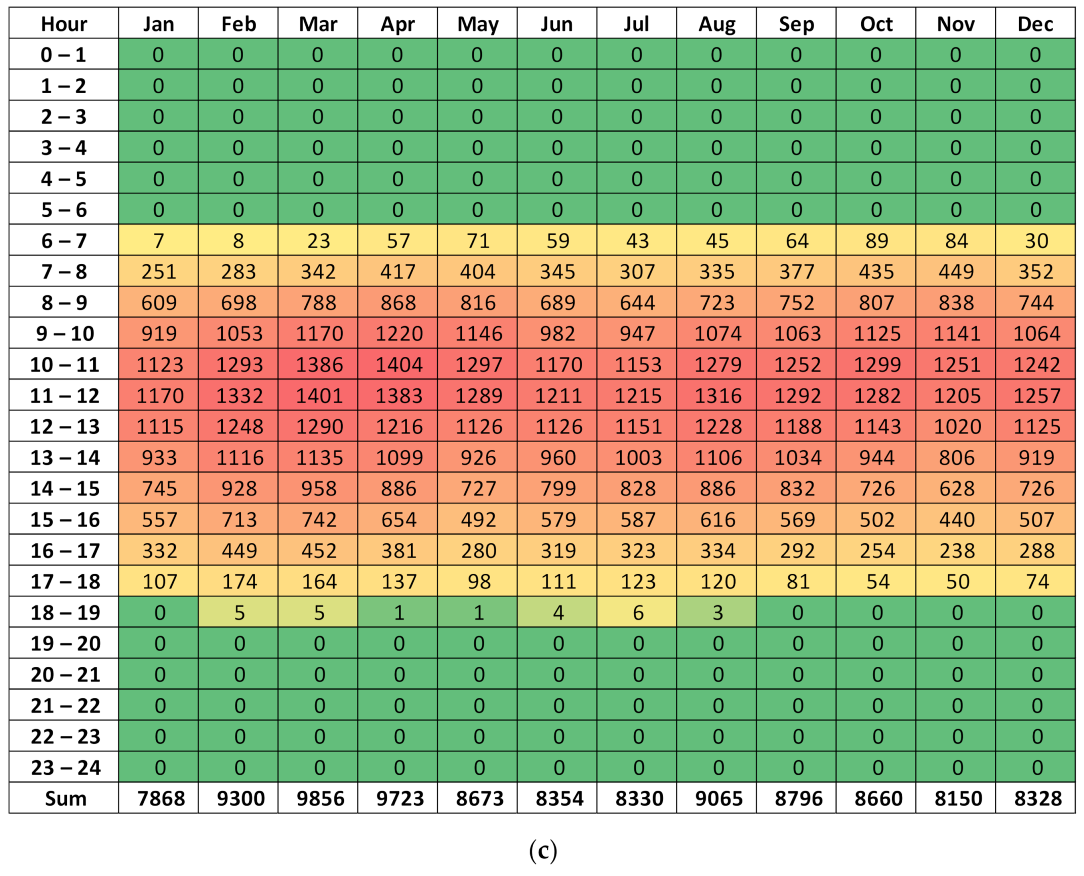
3.1. Photovoltaic Power Output
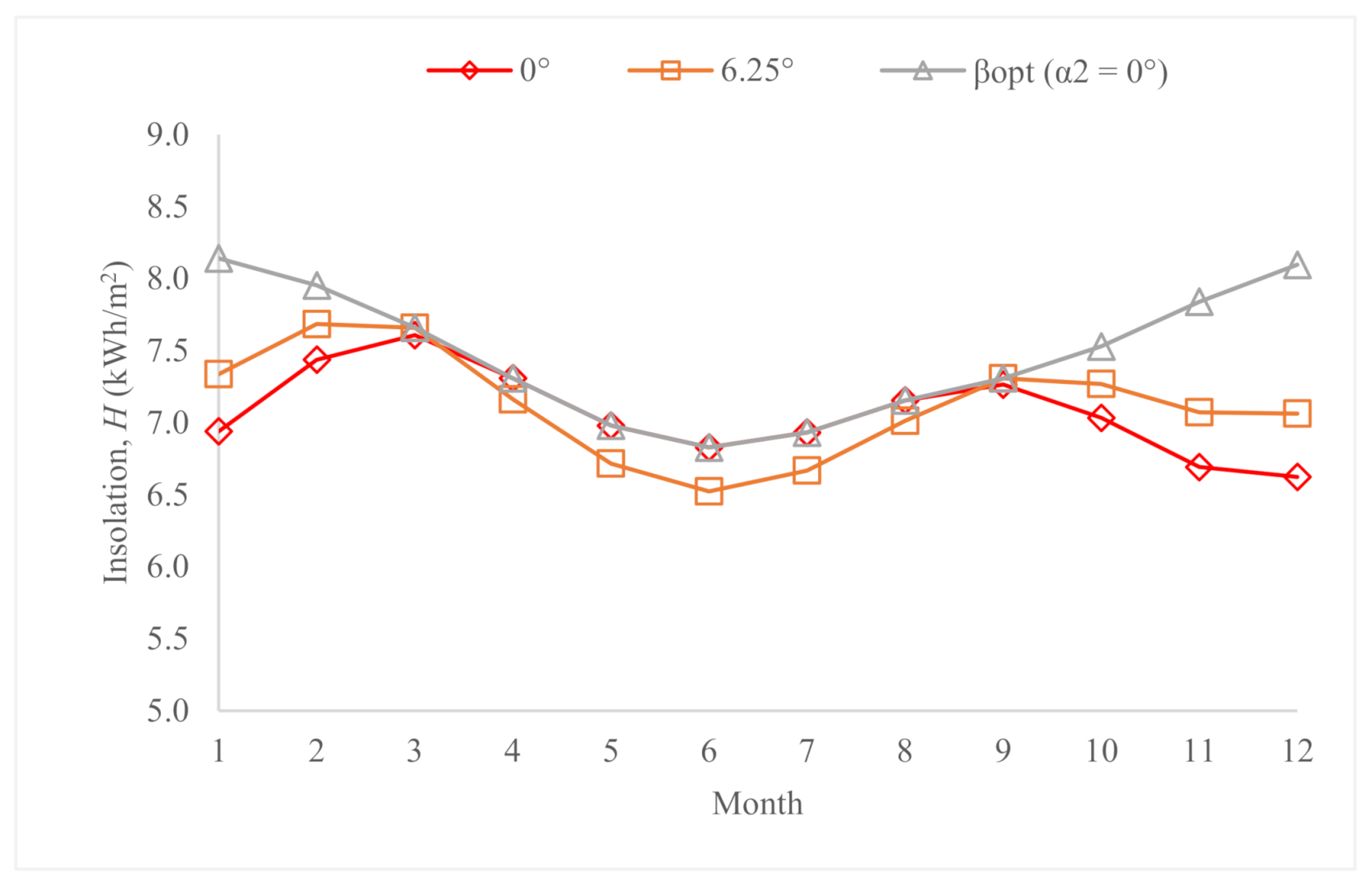
3.2. Collector Positioned at Variation of Tilt Angle with Fixed Orientation of Facing Due South
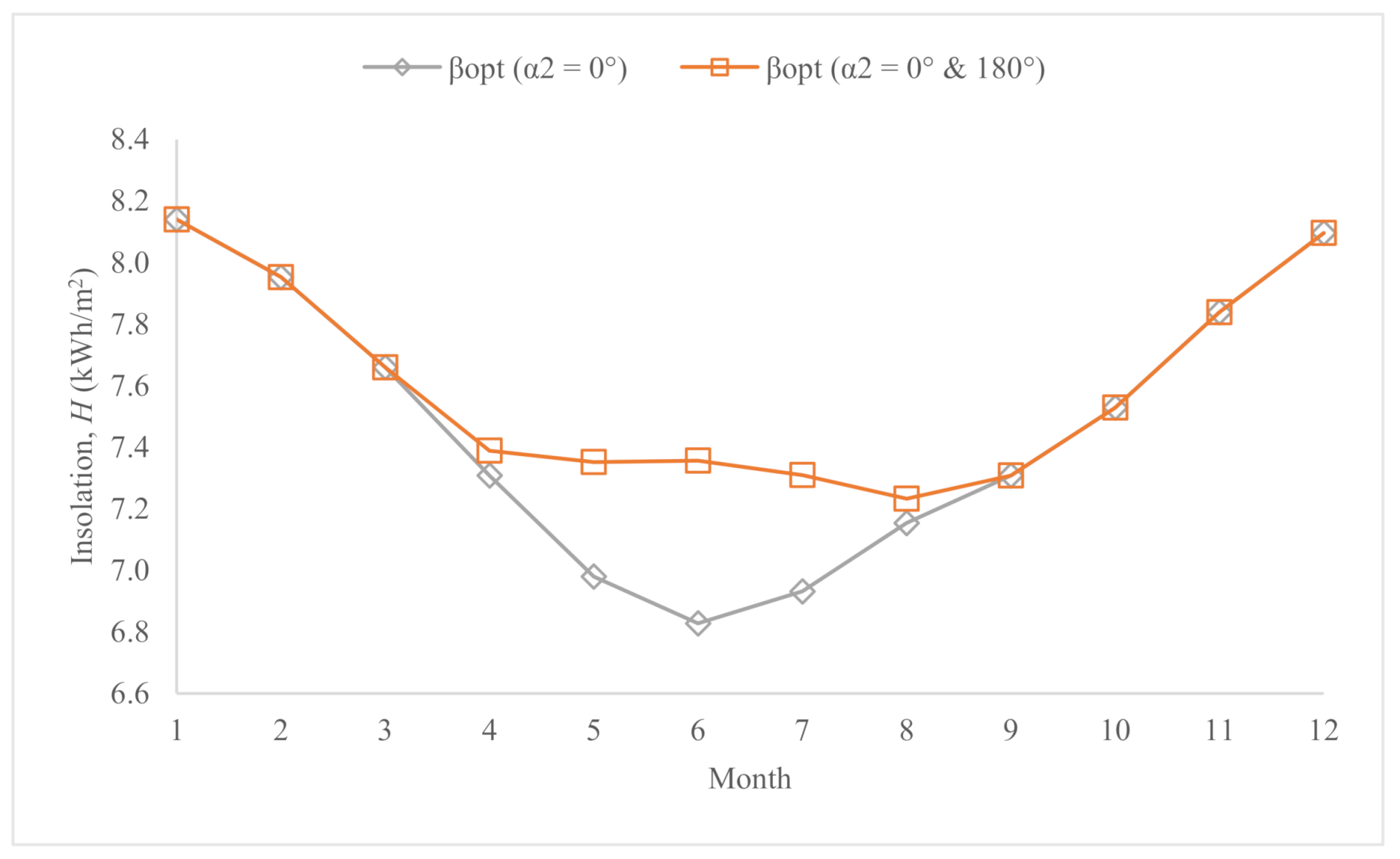
3.3. Collector Positioned at Optimum Tilt Angle with Variation of Orientation
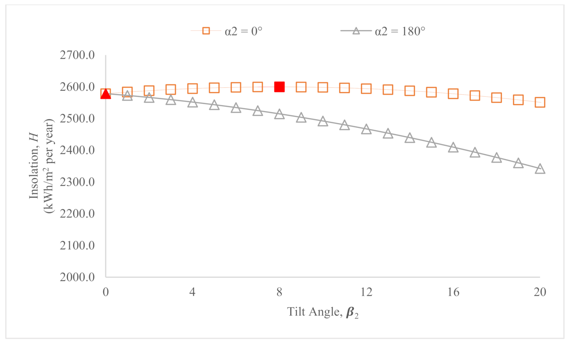
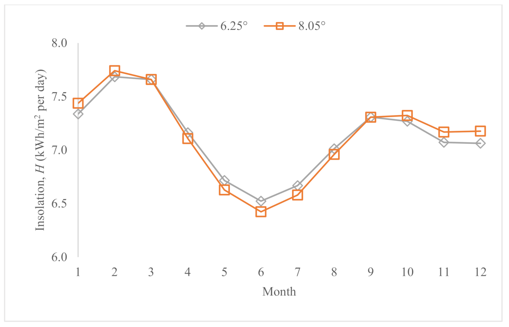
3.4. Collector Positioned at Fixed Tilt Angle and Variation of Orientation
4. Conclusions
- The Tian isotropic model is the preferred way for approximating insolation. It has been proven to have the lowest difference among all models, and it has a close agreement with the result of the optimum tilt angle provided by GSA 2.3.
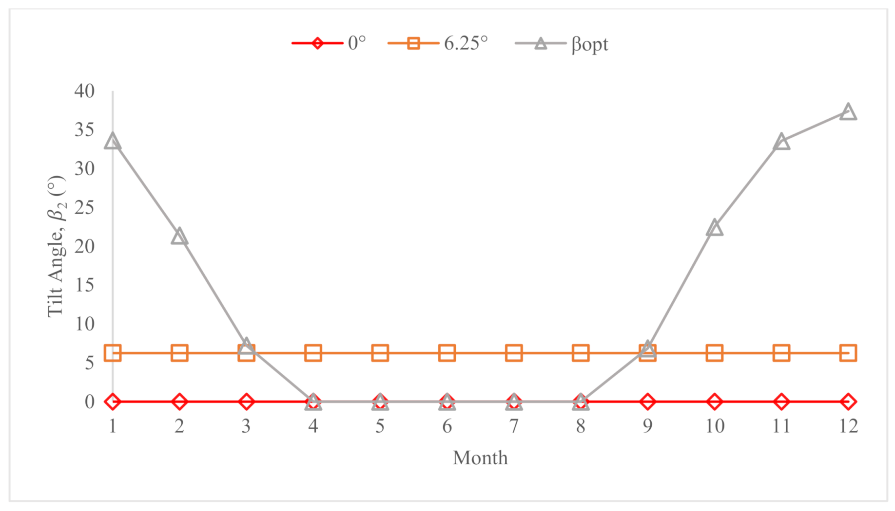
- In the condition where the collector’s orientation is kept in facing due south position throughout the year, the collector should be tilted at various values of according to the month of the year (Section 3.2).
- Meanwhile, in the condition where both the tilt angle and orientation could be adjusted throughout the year, (α2 = 0° and 180°) could provide maximum insolation (Section 3.3).
- The collector should be positioned at = 8.05° if the conditions of both the tilt angle and orientation (facing due south) are fixed.
- Lastly, in the case where the collector needs to be fixed facing due south from January to March and from September to December, and facing due north from April to August at EPLISSI, the collector tilt angle of = 24 ( = 0, i.e., south) and = 17 ( = 180, i.e., north), respectively, should be used.
- As verified in the study, the difference in PV power output data between the empirical models and GSA 2.3 (online PV simulation model) is considered acceptable. Without the comprehensive weather data similar to those being used in Solargis, an error in the order of 30% (in the range of 31% to 32%) should be expected, as shown in the data presented from Section 3.1.
Author Contributions
Funding
Institutional Review Board Statement
Informed Consent Statement
Data Availability Statement
Acknowledgments
Conflicts of Interest
Nomenclature
| A | Area of a circle |
| Radius of a circle | |
| Solar power | |
| Solar constant | |
| Optimum tilt angle | |
| δ | Declination Angle |
| N | Day number of year |
| L | Latitude |
| Long | Longitude |
| AST | Apparent solar time |
| LST | Local standard time |
| LSTM | Local standard time meridian |
| ET | Equation of time |
| h | Hour angle |
| Total solar irradiance | |
| ID | Direct irradiance |
| IDN | Direct normal irradiance |
| IS | Diffuse irradiance or sky radiation |
| IR | Reflected irradiance |
| Atmospheric pressure relative to a standard atmosphere | |
| z | Elevation |
| A | Apparent solar irradiation or apparent extra-terrestrial solar intensity |
| B | Atmospheric extinction coefficient |
| C | Ratio of diffuse radiation on a horizontal surface to direct normal irradiation |
| Foreground reflectivity | |
| H | Insolation |
| Total solar energy | |
| Acollector | Surface area of a collector |
| Total electrical energy | |
| Solar cell efficiency | |
| Ratio of the average daily diffuse radiation on a tilted surface to that on a horizontal surface | |
| Greek Symbols | |
| Solar altitude angle | |
| Collector or module tilt angle | |
| Solar azimuth angle | |
| Azimuth angle of the normal to the collector surface | |
| Collector angle |
References
- Seshie, Y.M.; N’Tsoukpoe, K.E.; Neveu, P.; Coulibaly, Y.; Azoumah, Y.K. Small scale concentrating solar plants for rural electrification. Renew. Sustain. Energy Rev. 2018, 90, 195–209. [Google Scholar] [CrossRef]
- U.S. Energy Information Administration. Today in Energy. 2017. Available online: https://www.eia.gov/todayinenergy/detail.php?id=33812 (accessed on 11 October 2020).
- International Energy Agency. The Latest Trends in Energy and Emissions in 2018; Global Energy and CO2 Status Report 2019; International Energy Agency: Paris, France, 2019. [Google Scholar]
- International Energy Agency. Global Energy Review 2020—The Impacts of the Covid-19 Crisis on Global Energy Demand and Carbon Dioxide Emissions. 2020. Available online: https://www.iea.org/reports/global-energy-review-2020/renewables (accessed on 11 October 2020).
- Shahzad, U. The need for renewable energy sources. Inform. Technol. Electr. Eng. 2015, 4, 16–19. [Google Scholar]
- Gielen, D.; Boshell, F.; Saygin, D.; Bazilian, M.D.; Wagner, N.; Gorini, R. The role of renewable energy in the global energy transformation. Energy Strategy Rev. 2019, 24, 38–50. [Google Scholar] [CrossRef]
- Malkawi, D.S.; Tamimi, A.I. Comparison of phase change material for thermal analysis of a passive hydronic solar system. J. Energy Storage 2021, 33, 102069. [Google Scholar] [CrossRef]
- Punniakodi, B.M.S.; Senthil, R. A review on container geometry and orientations of phase change materials for solar thermal systems. J. Energy Storage 2021, 36, 102452. [Google Scholar] [CrossRef]
- Da Rosa, A.V.; Ordóñez, J.C. Chapter 14—Photovoltaic converters. In Fundamentals of Renewable Energy Processes, 4th ed.; Academic Press: Oxford, UK, 2021; pp. 629–718. [Google Scholar]
- Oró, E.; Gil, A.; Gracia, A.; Boer, D.; Cabeza, L.F. Comparative life cycle assessment of thermal energy storage systems for solar power plants. Renew. Energy 2012, 44, 7. [Google Scholar] [CrossRef]
- Jayaraman, K.; Paramasivan, L.; Kiumarsi, S. Reasons for low penetration on the purchase of photovoltaic (PV) panel system among Malaysian landed property owners. Renew. Sustain. Energy Rev. 2017, 80, 562–571. [Google Scholar] [CrossRef]
- Renewable Energy Policy Network for the 21st Century. In Renewables 2019 Global Status Report; REN21: Paris, France, 2019.
- Parikh, A. Share of Solar & Wind Rose Despite Depressed Global Power Demand Amid Pandemic: IEA. 2020. Available online: https://mercomindia.com/share-of-solar-and-wind-rose/ (accessed on 11 October 2020).
- Saidur, R.; Jazi, G.B.; Mekhlif, S.; Jameel, M. Exergy analysis of solar energy applications. Renew. Sustain. Energy Rev. 2012, 16, 7. [Google Scholar] [CrossRef]
- Energysage. Should You Install a Solar Battery for Home Use? 2020. Available online: https://www.energysage.com/solar/solar-energy-storage/benefits-of-solar-batteries/ (accessed on 4 May 2021).
- Samsudin, M.S.N.; Rahman, M.M.; Wahid, M.A. Power generation sources in malaysia: Status and prospects for sustainable development. Adv. Rev. Sci. Res. 2016, 25, 18. [Google Scholar]
- Ahmad, N.A.; Byrd, H. Empowering distributed solar PV energy for Malaysian rural housing: Towards energy security and equitability of rural communities. Int. J. Renew. Energy Dev. 2013, 2, 10. [Google Scholar] [CrossRef]
- Halabi, L.M.; Mekhilef, S.; Olatomiwa, L.; Hazelton, J. Performance analysis of hybrid PV/diesel/battery system using HOMER: A case study Sabah, Malaysia. Energy Convers. Manag. 2017, 144, 18. [Google Scholar] [CrossRef]
- Izadyar, N.; Ong, H.C.; Chong, W.T.; Mojumder, J.C.; Leong, K.Y. Investigation of potential hybrid renewable energy at various rural areas in Malaysia. J. Clean. Prod. 2016, 139, 13. [Google Scholar] [CrossRef]
- Jäger, K.; Isabella, O.; Smets, A.H.M.; Swaaij, R.A.C.M.M.V.; Zeman, M. Solar Energy Fundamentals, Technology, and Systems; UIT Cambridge: Cambridge, UK, 2014. [Google Scholar]
- Salameh, T.; Abdelkareem, M.A.; Olabi, A.G.; Sayed, E.T.; Al-Chaderchi, M.; Rezk, H. Integrated standalone hybrid solar PV, fuel cell and diesel generator power system for battery or supercapacitor storage systems in Khorfakkan, United Arab Emirates. Int. J. Hydrog. Energy 2021, 46, 6014–6027. [Google Scholar] [CrossRef]
- Burke, M.J.; Stephens, J.C. Political power and renewable energy futures: A critical review. Energy Res. Soc. Sci. 2018, 35, 78–93. [Google Scholar] [CrossRef]
- Ho, S.; Abraham, L.; Edmund, C.O.; Urrego, L.R. Investigation of solar energy: The case study in Malaysia, Indonesia, Colombia and Nigeria. Int. J. Renew. Energy Res. 2019, 9, 10. [Google Scholar]
- Markos, F.M.; Sentian, J. Potential of solar energy in Kota Kinabalu, Sabah: An estimate using a photovoltaic system model. J. Phys. 2016, 710, 11. [Google Scholar] [CrossRef]
- World Bank Group. Global Solar Atlas Report Kota Belud. 2019. Available online: https://globalsolaratlas.info/map (accessed on 11 October 2020).
- Global Solar Atlas. Map and Data Downloads. Available online: https://globalsolaratlas.info/download/malaysia (accessed on 20 November 2020).
- Abdallah, R.; Juaidi, A.; Salameh, A.F.; Agugliaro, F.M. Estimating the optimum tilt angles for south-facing surfaces in Palestine. Energies 2020, 13, 623. [Google Scholar] [CrossRef]
- Awasthi, A.; Shukla, A.K.; Murali Manohar, S.R.; Dondariya, C.; Shukla, K.N.; Porwal, D.; Richhariya, G. Review on sun tracking technology in solar PV system. Energy Rep. 2020, 6, 392–405. [Google Scholar] [CrossRef]
- Khatib, T.; Muhsen, D.H. Optimal sizing of standalone photovoltaic system using improved performance model and optimisation algorithm. Sustainability 2020, 12, 2233. [Google Scholar] [CrossRef]
- Kasirajan, S.; Tan, K.T.; Leong, W.Y. Investigation on tilt angle calculation and irradiation on solar panels. Int. J. Eng. Technol. 2019, 8, 75–78. [Google Scholar]
- Office of Energy Efficiency and Renewable Energy. Solar Radiation Basics. 2020. Available online: https://www.energy.gov/eere/solar/solar-radiation-basics (accessed on 5 May 2021).
- Li, D.; Lam, T. Determining the optimum tilt angle and orientation for solar energy collection based on measured solar radiance data. Int. J. Photoenergy 2007, 8, 85402. [Google Scholar] [CrossRef]
- Shukla, K.N.; Rangnekarb, S.; Sudhakar, K. Comparative study of isotropic and anisotropic sky models to estimate solar radiation incident on tilted surface: A case study for Bhopal, India. Energy Rep. 2015, 1, 96–103. [Google Scholar] [CrossRef]
- Hailu, G.; Fung, A.S. Optimum tilt angle and orientation of photovoltaic thermal system for application in greater Toronto area, Canada. Sustainability 2019, 11, 6443. [Google Scholar] [CrossRef]
- Kamali, G.A.; Moradi, I.; Khalili, A. Estimating solar radiation on tilted surfaces with various orientations: A study case in Karaj (Iran). Theor. Appl. Climatol. 2006, 84, 235–241. [Google Scholar] [CrossRef]
- Mian, G.; Haixiang, Z.; Shengyu, G.; Tingji, C.; Jing, X.; Lexiang, C.; Zhinong, W.; Guoqiang, S. Optimal tilt angle and orientation of photovoltaic modules using HS algorithm in different climates of China. Appl. Sci. 2017, 7, 1028. [Google Scholar]
- Hertzog, P.E.; Swart, A.J. Optimum tilt angles for PV modules in a semi arid region of the Southern hemisphere. Int. J. Eng. Technol. 2018, 7, 290–297. [Google Scholar] [CrossRef]
- Soulayman, S.; Mohammad, M.; Salah, N. Solar receivers optimum tilt angle at southern hemisphere. Open Access Lib. J. 2016, 3, 1. [Google Scholar] [CrossRef]
- Khatib, T.; Mohamed, A.; Mahmoud, M.; Sopian, K. Optimisation of the tilt angle of solar panels for Malaysia. Energy Sour. 2015, 37, 606–613. [Google Scholar] [CrossRef]
- Khai, M.N.; Nor Mariah, A.; Othman, I.; Mohd Zainal Abidin, A.K. Assessment of solar radiation on diversely oriented surfaces and optimum tilts for solar absorbers in Malaysian tropical latitude. Int. J. Energy Environ. Eng. 2014, 5, 1–13. [Google Scholar]
- Fadaeenejad, M.; Mohd Amran, M.R.; Fadaeenejad, M.; Mahdi, Z.; Zohreh, G. Optimisation and comparison analysis for application of PV panels in three villages. Energy Sci. Eng. 2014, 3, 145–152. [Google Scholar] [CrossRef]
- Muhida, R.M.A.; Kassim, J.P.S.; Eusuf, M.A.; Sutjipto, A.G.; Afzeri, A. A simulation method to find the optimal design of photovoltaic home system in Malaysia, case study: A building integrated photovoltaic in Putra Jaya. World Acad. Sci. Eng. Technol. 2009, 53, 694–698. [Google Scholar]
- Sunderan, P.; Adibah, M.I.; Singh, B.; Norani, M.M. Optimum tilt angle and orientation of stand-alone photovoltaic electricity generation systems for rural electrification. Appl. Sci. 2011, 11, 1219–1224. [Google Scholar] [CrossRef]
- Elhassan, Z.A.M.; Zain, M.F.M.; Sopian, K.; Awadalla, A. Output energy of photovoltaic module directed at optimum slope angle in Kuala Lumpur, Malaysia. Appl. Sci. 2011, 6, 104–109. [Google Scholar] [CrossRef]
- Daut, M.I.I.; Irwan, Y.M.; Gomesh, N.; Rosnazri, N.S. Clear sky global solar irradiance on tilt angles of photovoltaic module in Perlis, Northern Malaysia. In Proceedings of the International Conference on Electrical, Control and Computer Engineering, Kuantan, Malaysia, 21–22 June 2011. [Google Scholar]
- Khatib, T.; Mohamed, A.; Sopian, K. Optimisation of a PV/wind micro-grid for rural housing electrification using a hybrid iterative/genetic algorithm: Case study of Kuala Terengganu, Malaysia. Energy Build. 2012, 47, 321–331. [Google Scholar] [CrossRef]
- Omidreza, S.K.S.; Elhab, B.; Ruslan, M.H.; Asim, N. Optimal solar panels’ tilt angles and orientations in Kuala Lumpur, Malaysia. In Proceedings of the 1st WSEAS International Conference on Energy and Environment Technologies and Equipment (EEETE’ 12), Zlin, Czech Republic, 20–22 September 2012. [Google Scholar]
- Hussein, A.K.; Miqdam, T.C.; Ali, H.A.; Kavish, M. Effect of shadow on the performance of solar photovoltaic. In Mediterranean Green Buildings & Renewable Energy; Springer: Cham, Switzerland, 2015. [Google Scholar]
- Weather Spark. Average Weather in Kota Belud, Malaysia. Available online: https://weatherspark.com/y/130293/Average-Weather-in-Kota-Belud-Malaysia-Year-Round (accessed on 19 November 2020).
- World Weather Online. Kota Belud Monthly Climate Averages. Available online: https://www.worldweatheronline.com/kota-belud-weather-averages/sabah/my.aspx (accessed on 19 November 2020).
- Solargis. Methodology—Solar Radiation Modeling. Available online: https://solargis.com/docs/methodology/solar-radiation-modeling (accessed on 3 May 2021).
- Ineichen, P. Long Term Satellite Hourly, Daily and Monthly Global, Beam and Diffuse Irradiance Validation. Interannual Variability Analysis; Adapted to CM-SAF Product from the IEA 2013 Report; IEA: Paris, France, 2014. [Google Scholar]
- Global Solar Atlas. About Global Solar Atlas. Available online: https://globalsolaratlas.info/support/about (accessed on 15 October 2020).
- Solargis. Documentation: Methodology. Available online: https://solargis.com/docs/methodology (accessed on 4 May 2021).
- Duffie, J.; Beckman, W. Solar Engineering of Thermal Processes, 2nd ed.; John Wiley and Sons: New York, NY, USA, 1991. [Google Scholar]
- Hagen, K.D. Introduction to Renewable Energy for Engineers; Pearson: London, UK, 2016. [Google Scholar]
- Holbert, K.E. Solar Calculations. 2007. Available online: http://holbert.faculty.asu.edu/eee463/SolarCalcs.pdf (accessed on 11 October 2020).
- Lunde, P.J. Solar Thermal Engineering Space Heating and Hot Water Systems; John Wiley and Sons: New York, NY, USA, 1980. [Google Scholar]
- Liu, B.Y.H.; Jordan, R.C. The Interrelationship and Characteristic Distribution of Direct, Diffuse, and Total Solar Radiation. Solar Energy 1960, 4, 1–19. [Google Scholar] [CrossRef]
- Kotak, Y.; Gul, M.; Muneer, T.; Ivanova, S. Investigating the impact of ground albedo on the performance of PV systems. In Proceedings of the CIBSE Technical Symposium, London, UK, 16–17 April 2015. [Google Scholar]
- Koronakis, P.S. On the choice of the angle of tilt for south facing solar collectors in the Athens basin area. Solar Energy 1986, 36, 217–225. [Google Scholar] [CrossRef]
- Badescu, V. A new kind of cloudy sky model to compute instantaneous values of diffuse and global solar irradiance. Theor. Appl. Climatol. 2002, 72, 127–136. [Google Scholar] [CrossRef]
- Tian, Y.Q.; Davies-Colley, R.J.; Gonga, P.; Thorrold, B.W. Estimating solar radiation on slopes of arbitrary aspect. Agricult. For. Meteorol. 2001, 1, 67–74. [Google Scholar] [CrossRef]
- Richardson, L. How Long Do Solar Panels Last? 2020. Available online: https://news.energysage.com/how-long-do-solar-panels-last/ (accessed on 16 October 2020).


| Papers | Case Study | Monthly Optimum Angle | Optimum Fixed Tilt Angle | Applied Tool | Method | Orientation of PV |
|---|---|---|---|---|---|---|
| Khatib, Mohamed, Mahmoud, Sopian [39] | Kuala Lumpur, Ipoh, Alor Setar, Johor Bharu, and Kuching | Provided | latitude of the location | Excel | Liu and Jordan | South |
| Khai, Nor Mariah, Othman, Mohd Zainal [40] | Bangi | Provided | 14.4° ± 5° and 14.8° ± 5°—latitude of the location | MATLAB | KT solar radiation model | Facing south and north |
| Muhida [42] | Kuala Lumpur | - | 1° to 15° | Solar Pro | - | No difference |
| Sunderan [43] | Ipoh, Perak | Provided | 0° or tilt angle—latitude of the location | - | Collares—Pereira and Rabi | Facing south and north |
| Elhassan [44] | Kuala Lumpur | - | 15° to 30° | PVSYS-50, Excel, MATLAB | - | East, north |
| Daut [45] | Perlis | Provided | - | - | - | - |
| Khatib [46] | Kuala Terengganu | Provided | 0° to 23° | MATLAB | Liu and Jordan | - |
| Omidreza [47] | Kuala Lumpur | - | 10° | Excel | Cooper’s equation | - |
| Type of Demand | Energy Used, kWh |
|---|---|
| Total peak demand | 11.874 |
| Total average demand | 4.600 |
| Type of Foreground | |
|---|---|
| Corrugated roof | 0.10–0.15 |
| Coloured paint | 0.15–0.35 |
| Trees | 0.15–0.18 |
| Asphalt | 0.05–0.20 |
| Concrete | 0.25–0.70 |
| Grass | 0.25–0.30 |
| Ice | 0.30–0.50 |
| Month | Day Number of Year, N | Total Days |
|---|---|---|
| January (Jan) | 21 | 31 |
| February (Feb) | 52 | 28 |
| March (Mar) | 80 | 31 |
| April (Apr) | 111 | 30 |
| May (May) | 141 | 31 |
| June (June) | 172 | 30 |
| July (Jul) | 202 | 31 |
| August (Aug) | 233 | 31 |
| September (Sept) | 264 | 30 |
| October (Oct) | 294 | 31 |
| November (Nov) | 325 | 30 |
| December (Dec) | 355 | 31 |
| January (Jan) | 21 | 31 |
| Section | Orientation | |
|---|---|---|
| Section 3.2 | = 0 | |
| Section 3.3 | = 0 | |
| = 0 and 180 | ||
| Section 3.4 | = 0 | |
| = 180 |
| Type of Model | Optimum Tilt Angle, βopt |
|---|---|
| GSA 2.3 | 6 |
| Liu and Jordan | 8 |
| Koronakis | 8 |
| Badescu | 8 |
| Tian | 7 |
| Month | β2 = 0° | β2 = 6.25° | βopt (α2 = 0°) |
|---|---|---|---|
| 1 or Jan (N = 21) | 0° | 6.25° | 33.63° |
| 2 or Feb (N = 52) | 0° | 6.25° | 21.39° |
| 3 or Mar (N = 80) | 0° | 6.25° | 7.23° |
| 4 or Apr (N = 111) | 0° | 6.25° | 0° |
| 5 or May (N = 141) | 0° | 6.25° | 0° |
| 6 or June (N = 172) | 0° | 6.25° | 0° |
| 7 or Jul (N = 202) | 0° | 6.25° | 0° |
| 8 or Aug (N = 233) | 0° | 6.25° | 0° |
| 9 or Sept (N = 264) | 0° | 6.25° | 6.87° |
| 10 or Oct (N = 294) | 0° | 6.25° | 22.49° |
| 11 or Nov (N = 325) | 0° | 6.25° | 33.55° |
| 12 or Dec (N = 355) | 0° | 6.25° | 37.39° |
| Month | Insolation, H (kWh/m2 Per Month) | ||
|---|---|---|---|
| β2 = 0° | β2 = 6.25° | βopt (α2 = 0°) | |
| 1 or Jan (N = 21) | 215.14 | 227.44 | 252.3504 |
| 2 or Feb (N = 52) | 208.24 | 215.17 | 222.6841 |
| 3 or Mar (N = 80) | 235.84 | 237.43 | 237.4567 |
| 4 or Apr (N = 111) | 219.25 | 214.88 | 219.2480 |
| 5 or May (N = 141) | 216.38 | 208.19 | 216.3801 |
| 6 or June (N = 172) | 204.84 | 195.69 | 204.8364 |
| 7 or Jul (N = 202) | 214.89 | 206.71 | 214.8856 |
| 8 or Aug (N = 233) | 221.77 | 217.39 | 221.7708 |
| 9 or Sept (N = 264) | 217.92 | 219.24 | 219.2497 |
| 10 or Oct (N = 294) | 218.05 | 225.34 | 233.3893 |
| 11 or Nov (N = 325) | 200.75 | 212.16 | 235.1755 |
| 12 or Dec (N = 355) | 205.32 | 218.96 | 250.9803 |
| Total insolation, H (kWh/m2 per year) | 2578.36 | 2598.60 | 2728.41 |
| Month | βopt (α2 = 0°) | H of βopt (α2 = 0°) (kWh/m2 Per Month) | βopt (α2 = 0° & 180°) | H of βopt (α2 = 0° & 180°) (kWh/m2 Per Month) |
|---|---|---|---|---|
| 1 or Jan (N = 21) | 33.63° | 252.35 | 33.63° | 252.35 |
| 2 or Feb (N = 52) | 21.39° | 222.68 | 21.39° | 222.68 |
| 3 or Mar (N = 80) | 7.23° | 237.46 | 7.23° | 237.46 |
| 4 or Apr (N = 111) | 0° | 219.25 | −9.21° | 221.66 |
| 5 or May (N = 141) | 0° | 216.38 | −20.00° | 227.91 |
| 6 or June (N = 172) | 0° | 204.84 | −23.93° | 220.69 |
| 7 or Jul (N = 202) | 0° | 214.89 | −20.31° | 226.60 |
| 8 or Aug (N = 233) | 0° | 221.77 | −9.29° | 224.22 |
| 9 or Sept (N = 264) | 6.87° | 219.25 | 6.87° | 219.25 |
| 10 or Oct (N = 294) | 22.49° | 233.39 | 22.49° | 233.39 |
| 11 or Nov (N = 325) | 33.55° | 235.18 | 33.55° | 235.18 |
| 12 or Dec (N = 355) | 37.39° | 250.98 | 37.39° | 250.98 |
| Total insolation, H (kWh/m2 per year) | - | 2728.41 | - | 2772.38 |
Publisher’s Note: MDPI stays neutral with regard to jurisdictional claims in published maps and institutional affiliations. |
© 2021 by the authors. Licensee MDPI, Basel, Switzerland. This article is an open access article distributed under the terms and conditions of the Creative Commons Attribution (CC BY) license (https://creativecommons.org/licenses/by/4.0/).
Share and Cite
Matius, M.E.; Ismail, M.A.; Farm, Y.Y.; Amaludin, A.E.; Radzali, M.A.; Fazlizan, A.; Muzammil, W.K. On the Optimal Tilt Angle and Orientation of an On-Site Solar Photovoltaic Energy Generation System for Sabah’s Rural Electrification. Sustainability 2021, 13, 5730. https://doi.org/10.3390/su13105730
Matius ME, Ismail MA, Farm YY, Amaludin AE, Radzali MA, Fazlizan A, Muzammil WK. On the Optimal Tilt Angle and Orientation of an On-Site Solar Photovoltaic Energy Generation System for Sabah’s Rural Electrification. Sustainability. 2021; 13(10):5730. https://doi.org/10.3390/su13105730
Chicago/Turabian StyleMatius, Maryon Eliza, Mohd Azlan Ismail, Yan Yan Farm, Adriana Erica Amaludin, Mohd Adzrie Radzali, Ahmad Fazlizan, and Wan Khairul Muzammil. 2021. "On the Optimal Tilt Angle and Orientation of an On-Site Solar Photovoltaic Energy Generation System for Sabah’s Rural Electrification" Sustainability 13, no. 10: 5730. https://doi.org/10.3390/su13105730
APA StyleMatius, M. E., Ismail, M. A., Farm, Y. Y., Amaludin, A. E., Radzali, M. A., Fazlizan, A., & Muzammil, W. K. (2021). On the Optimal Tilt Angle and Orientation of an On-Site Solar Photovoltaic Energy Generation System for Sabah’s Rural Electrification. Sustainability, 13(10), 5730. https://doi.org/10.3390/su13105730