Article

An Efficient Approach to Automatic Construction of 3D Watertight Geometry of Buildings Using Point Clouds

Department of Civil Engineering, Xi’an Jiaotong-Liverpool University, Suzhou 215123, China
*
Author to whom correspondence should be addressed.
Remote Sens. 2021, 13(10), 1947; https://doi.org/10.3390/rs13101947
Submission received: 9 April 2021 / Revised: 7 May 2021 / Accepted: 14 May 2021 / Published: 17 May 2021

Abstract

:
Recent years have witnessed an increasing use of 3D models in general and 3D geometric models specifically of built environment for various applications, owing to the advancement of mapping techniques for accurate 3D information. Depending on the application scenarios, there exist various types of approaches to automate the construction of 3D building geometry. However, in those studies, less attention has been paid to watertight geometries derived from point cloud data, which are of use to the management and the simulations of building energy. To this end, an efficient reconstruction approach was introduced in this study and involves the following key steps. The point cloud data are first voxelised for the ray-casting analysis to obtain the 3D indoor space. By projecting it onto a horizontal plane, an image representing the indoor area is obtained and is used for the room segmentation. The 2D boundary of each room candidate is extracted using new grammar rules and is extruded using the room height to generate 3D models of individual room candidates. The room connection analyses are applied to the individual models obtained to determine the locations of doors and the topological relations between adjacent room candidates for forming an integrated and watertight geometric model. The approach proposed was tested using the point cloud data representing six building sites of distinct spatial confirmations of rooms, corridors and openings. The experimental results showed that accurate watertight building geometries were successfully created. The average differences between the point cloud data and the geometric models obtained were found to range from 12 to 21 mm. The maximum computation time taken was less than 5 min for the point cloud of approximately 469 million data points, more efficient than the typical reconstruction methods in the literature.

1. Introduction

In recent years, the global interest in building energy efficiency has increased significantly [1,2]. For example, the Spanish government elaborated the “Integrated National Plan for Energy and Climate 2012–2030”, aiming for energy savings through the rehabilitation and improvement of the energy efficiency in existing buildings [3]. To fulfil this objective, energy simulations need to be performed for existing buildings, which require the knowledge of their as-built information. However, such information is often incomplete, obsolete or fragmented [4]. To this end, measurement techniques (e.g., laser scanning and photogrammetry) have been applied to obtain that type of information [5]. Although in the energy simulation tools dense triangular mesh reconstructed from the point cloud data can be used to model the thermodynamic properties of building interiors, such overly complex geometric models can hinder the performance of those tools [6]. Therefore, it is highly desirable to construct simple 3D geometric models constituted by structural objects (e.g., doors, walls, floors, ceilings, and columns) from the point cloud data.
Three-dimensional geometric models of building structures have widely been used in various applications such as indoor navigation guidance [7,8], the management of energy, space and emergency [9,10,11], health monitoring and retrofit planning [12,13,14], and risk management of the decommissioning processes [15,16,17,18] of buildings. Using point cloud data, researchers have proposed a variety of approaches to the automatic reconstruction of building structures [11,19,20,21,22,23,24]. In these approaches, there are mainly two steps in the process of the 3D geometric modelling for a building. The first step is to obtain an initial geometric model of the building, which is usually achieved by segmentations for building elements (e.g., walls, ceilings and floors) to obtain their shape representations. In the second step, the shape representations obtained are optimised to produce a final geometrical model of the building. The optimisation process may include various tasks, such as the connection of the shape representations of adjacent building elements, the merging of the shape representations which belong to the same building element, and the correction and deletion of any false shape representations.
Buildings often consist of geometric primitives with planar surfaces. Therefore, planes are usually the basic elements to build up an initial geometric model. Nurunnabi et al. [25] suggested that there were three commonly used methods for plane detection, including Random Sample Consensus (RANSAC), Principle Component Analysis (PCA) and least-squares. In general, both PCA and least-squares are sensitive to noisy data, whereas RANSAC can extract planes effectively even when there is a reasonably large amount of noisy data. Therefore, RANSAC and its variants have become the most popular types of methods [26]. Nurunnabi et al. [25] developed a tailored PCA, which was tested against other methods using a point cloud obtained with the mobile mapping technique. Their custom PCA solution was found to be faster than RANSAC and perform roughly equally in terms of accuracy of plane detection, but it was less tolerant to outliers. Along with the aforementioned methods, there are several other methods for plane detection, such as plane sweeping [27], surface normal approaches [28] and region growing [19].
However, without proper optimisation, the computational demand of RANSAC could be enormous when applying it to large-scale point clouds [26]. This has led to many extensions or variants to the original RANSAC method [29]. One of the most influential variants was proposed by Schnabel et al. [26], which takes account of the deviation of the normals between the candidate shape and the point cloud data used. Similar to Schnabel et al. [26], the work of Rusu et al. [30] added the surface normal constraints for the optimisation. It was found that in their scene approximately 85% of surface normals had a principal direction that was along with one of the Cartesian axes (X, Y or Z). The segmentation was performed on a sub-set of the whole point cloud, and was focused on horizontal planes where the normals are parallel to the Z direction and vertical planes where they are perpendicular to each other. The planar areas identified were broken into smaller parts with region growing, which used the Euclidean distances and the changes in curvatures between data points as the parameters for inlier addition. Machine learning (i.e., Conditional Random Fields) was then used to classify the shapes as objects.
Pu and Vosselman [31] used the surface region growing segmentation for categorising the data points representing building facades into regions with planar surfaces, followed by the application of constraint rules (such as size, position, direction) to optimise the segmentation results. It was found that better results could be achieved by hierarchically detecting building elements according to certain rules.
Numerous approaches have been proposed to optimise initial geometric models for a final integrated 3D geometric model, which can be divided into two categories. The first category consists of data-driven methods, including local and global methods [32,33,34]. Local data-driven methods focus on acquiring the best-fitted geometric models in a local scale. In these types of methods, the characteristics (e.g., surface normals, surface curvatures and point densities) of the point cloud data within a local scale (e.g., a local segmented plane) are used for model optimisation [20,35,36]. In the global methods, a geometric model is optimised using global-scale criteria such as the maximisation of the spatial coverage of data or the total internal space of the geometric model. In general, local data-driven approaches are susceptible to occlusion [20,37]. Therefore, in order to obtain satisfactory 3D geometric models, high-quality data are often required. Otherwise, additional efforts are required to resolve the occlusion-induced issues. For example, occlusion detection and the inpainting algorithms were used by Xiong et al. [37] to detect and reconstruct the missing points due to occlusion. In contrast, since global data-driven approaches are optimised for the global scale criteria, they are less dependent on data quality. However, there are other negative effects. A common one is that the local details are prone to be lost during the global optimisation process, although this could be solved by manually adding constraints for the reconstruction.
In the second category of geometry optimization, shape grammars were considered, which are based mainly on the architectural design principles and the structural arrangements [38,39]. The grammar-based approaches were initially adopted for urban reconstruction (e.g., building facade reconstruction) [40,41,42] and were later applied to indoor environment reconstruction too [22,43]. The grammar-based approaches are less susceptible to imperfect data compared to the data-driven ones [22,43]. However, they usually require manual definitions of grammar rules, application orders and parameters. In addition, because extracting usable shape grammars for irregular structures (e.g., with inclined walls or with walls intersecting at random angles) is extremely difficult, these approaches can be adopted mainly for regular grid-like buildings (e.g., the Manhattan world) [22,43].
Unlike data-driven methods, grammar-based approaches use architectural design principles to identify and to refine the widely applicable shape grammars for grid-like structures [44,45,46,47,48,49,50,51,52,53,54,55,56]. The early-stage grammars for indoor environment modelling came from virtual environment research. Boulch et al. [52] proposed a method to interpret the semantic information of a 3D geometric model with grammars. They tested this approach on both CAD models, simulated indoor point clouds and real point clouds of building exteriors. In their approach, the point clouds were first segmented into planar clusters using grammars, and objects were detected and recognized using the planar clusters obtained. Overall, Boulch et al. [52] suggest that grammars could be simple rules but the approach may become complex when grammars are combined. There are two main advantages of the grammar-based approaches: (1) they are less susceptible to occlusion and noise [52], and (2) the accurate topological information between reconstructed structural components can easily be obtained [22,39]. Such information lets the geometric models constructed be readily compatible with indoorGML and Industry Foundation Classes (IFC). However, the current grammar-based approaches usually require a manual establishment of grammar rules, which is a time-consuming process. Moreover, those shape grammars are applicable mainly for simple and regular structures such as the Manhattan world building.
In the aforementioned approaches, a range of factors and information were often taken into account to maximise their generalisation in modelling complex geometries, which lead to complicated reconstruction processes and hence often become less computationally efficient. Furthermore, as they were not specifically developed for the applications in energy management and simulations of building structures, they did not intentionally honour the two fundamental requirements in such applications [11]. More specifically, the requirements consist of watertight geometries and accurate partitions of the indoor space to represent distinct thermal zones [6]. For example, the approaches in Bassier and Vergauwen [54] and Sanchez et al. [24] led to non-watertight geometric models that are unsuitable for energy simulations.
The main purpose of this study is to investigate an efficient approach to construct watertight geometric models (of the Manhattan world structures). To this end, new grammar rules were proposed and used along with some image processing techniques and the topology analysis to generate watertight geometric models with interior doors and segmented rooms.

2. Materials and Methods

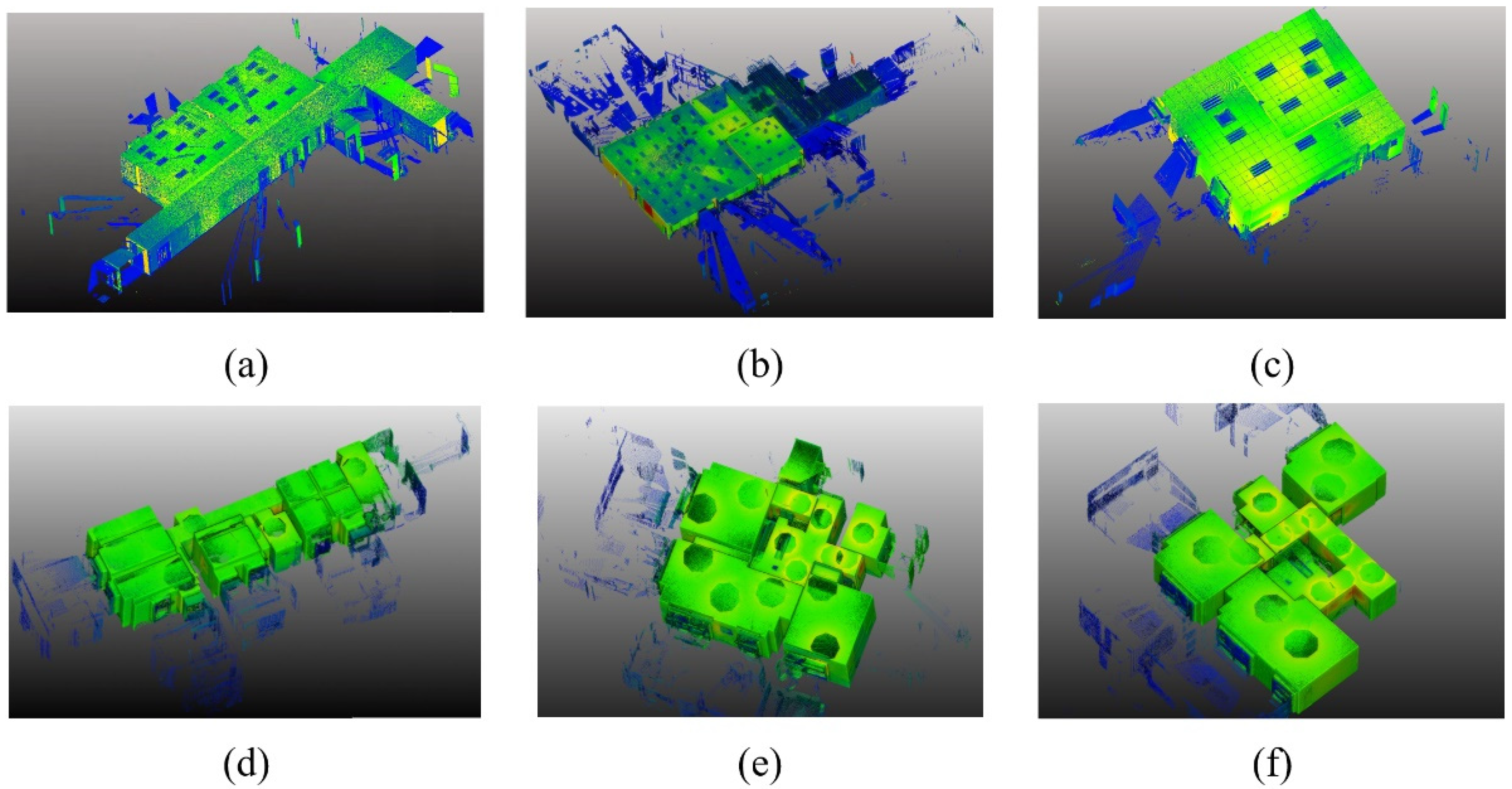
2.1. Study Sites and Data
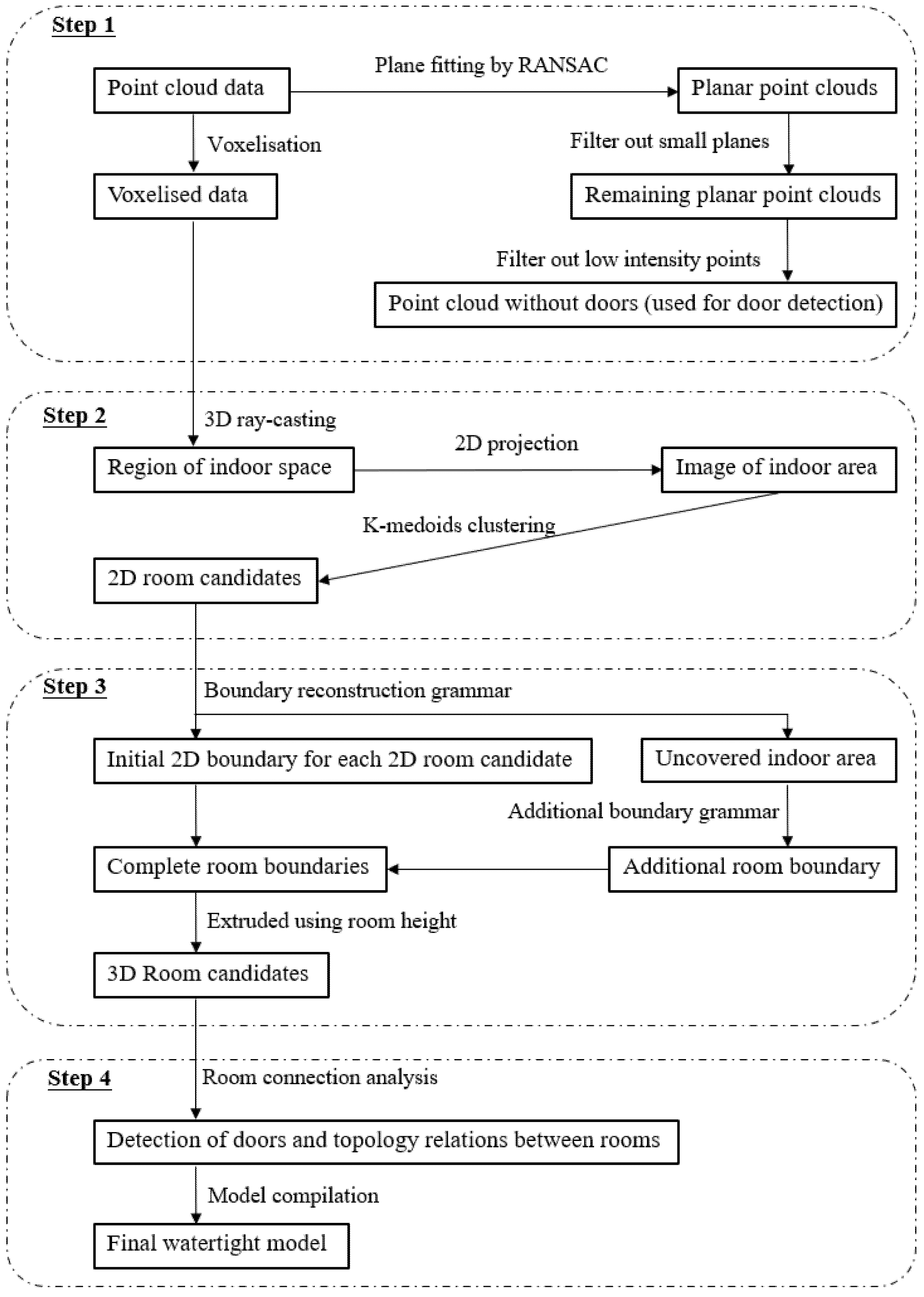
Parts of several campus buildings and three residential apartments were selected as the study sites. These sites represent different spatial arrangements of room components, including rooms of various sizes, corridors and openings. In Site 3, there are high occlusions due to the cabinets placed against the walls. Sites 1–3 were surveyed from multiple scan stations using a Leica RTC360 scanner. The point cloud data obtained from each station were aligned initially by the scanner during the surveying campaigns, which was followed by a refined registration using the Leica Cyclone software. The data of Sites 4–6 were obtained from the online source [57], and were acquired using a RGBD camera (i.e., Matterport). Similar to RTC360, Matterport is able to rotate horizontally around a centre and automatically captures a panoramic depth image, which can easily be transformed into point cloud data. The registered point clouds for these sites considered are shown in Figure 1, which consist of approximately 476 million, 469 million, 40 million, 4.93 million, 4.53 million, and 4.22 million data points, respectively. To estimate the positional accuracy of the data points obtained from the laser scanner and the RGBD camera, the plane encompassing the maximum number of data points for each dataset was fitted by the RANSAC algorithm, followed by the calculation of the point-to-plane distances. The mean and standard deviation of the point-to-plane distances for datasets 1–3 combined are 0.11 mm and 0.26 mm, respectively, while for datasets 4–6 combined these two values are 1.45 mm and 6.69 mm, respectively.

2.2. Methodology

The existing reconstruction approaches can be plane-fitting based or contour-based. The former is based on the observation that the majority of building structures are composed of planar parts [11], while the latter assumes that the indoor scenes have a 2.5D structure [46,55,56]. Since the contour-based approaches mainly involve the processing of 2D data, they are inherently simpler and are thus considered in conjunction with some reconstruction grammars in this study. Furthermore, compared to unorganised 2D data (i.e., the XY coordinates of point cloud data), gridded data such as images are often easier to be handled. As such, in this study, the unorganised 2D data were gridded into images and were processed using some well-developed image processing techniques. The key steps of the approach investigated are illustrated in the flowchart in Figure 2 and are elaborated in the following sections.

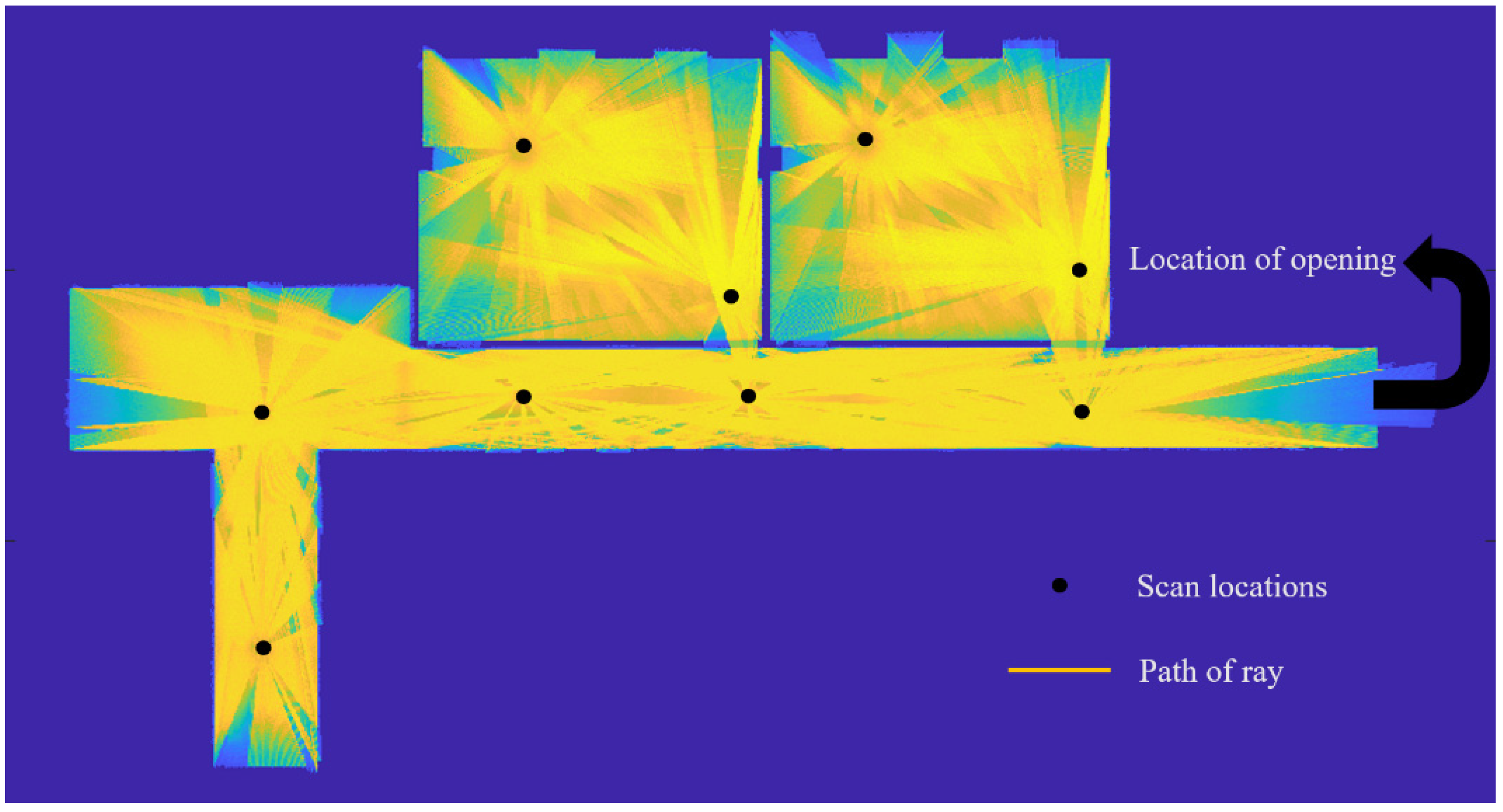
2.2.1. Pre-Processing (Step 1)

To better adapt to the image processing techniques used in the subsequent steps and to reduce the computational cost, the original point cloud data were voxelised in the first place. The bounding box of the whole point cloud was set to be the space for voxelisation. For each voxel inside the space, it was labelled as empty when it did not contain any data point and otherwise labelled as occupied. In this study, the voxel size was set to be 12 mm, which was adequate for producing accurate final geometric models.
In the approach proposed, openings on the walls were checked using grammars to determine if they are doors. To facilitate this, the point cloud data representing partially or fully closed doors were identified and removed. As illustrated in Figure 3, closed doors may either be located at a small distance from the wall (non-coplanar, Case a in Figure 3) or be coplanar with the wall (Case b in Figure 3). The filtering rules applied are presented in the following.
Firstly, vertical planes were fitted to the point cloud data obtained at each scanner station using RANSAC [26]. Afterwards, the point cloud data representing the vertical planes with a height less than 0.9 times the room height were classified as potential non-coplanar doors and removed. This was found to be an effective and efficient means of removing non-coplanar doors.
However, a more sophisticated method was needed to remove the data points representing coplanar doors. To achieve this, a moving window was used to analyse the intensity histograms of the data points. As the reflectance of the doors is different from that of the walls, the intensity histogram of a local area containing a door typically has two local peaks in the histogram, as shown in Figure 4a. The coplanar doors were removed by filtering out the data points in the lower peak region of the histogram in this study, as illustrated in Figure 4b. More specifically, for each remaining vertical plane (excluding those being deleted as non-coplanar doors), a 3.5 m wide window with a height being the same as the plane height was moved from one end of the plane to the other along its horizontal principal direction at an interval of 3.5 m (i.e., the width of the window). The data points in the lower peak were deleted when the number of them was less than 75% of the total number of data points inside the moving window. It is worth mentioning that the width of the moving window was determined through a set of tests, which aim to find an appropriate width for the moving window to provide a similar intensity histogram for regions with the door. In the tests, when the size of the moving window was smaller than the door (typically 2 m), it was difficult to define simple criteria to filter out the data points representing the doors because the intensity histograms of the data in the window would have various cases, as shown in Figure 5. Especially when the moving window was inside the door, the percentage of points in the lower peak depended on the ratio between the door height and the plane height, which could vary from one site to another. Therefore, the width of the moving window at least should be larger than the typical door width (i.e., 2 m), while the final width of 3.5m was ascertained by trial-and-error.
Although the aforementioned rules can effectively remove the data representing the doors, data points associated with some small planes representing other objects might also be removed in the process. This did not affect the model constructed as the filtered data were used only for the door detection process in the room connection analysis (i.e., Step 4).

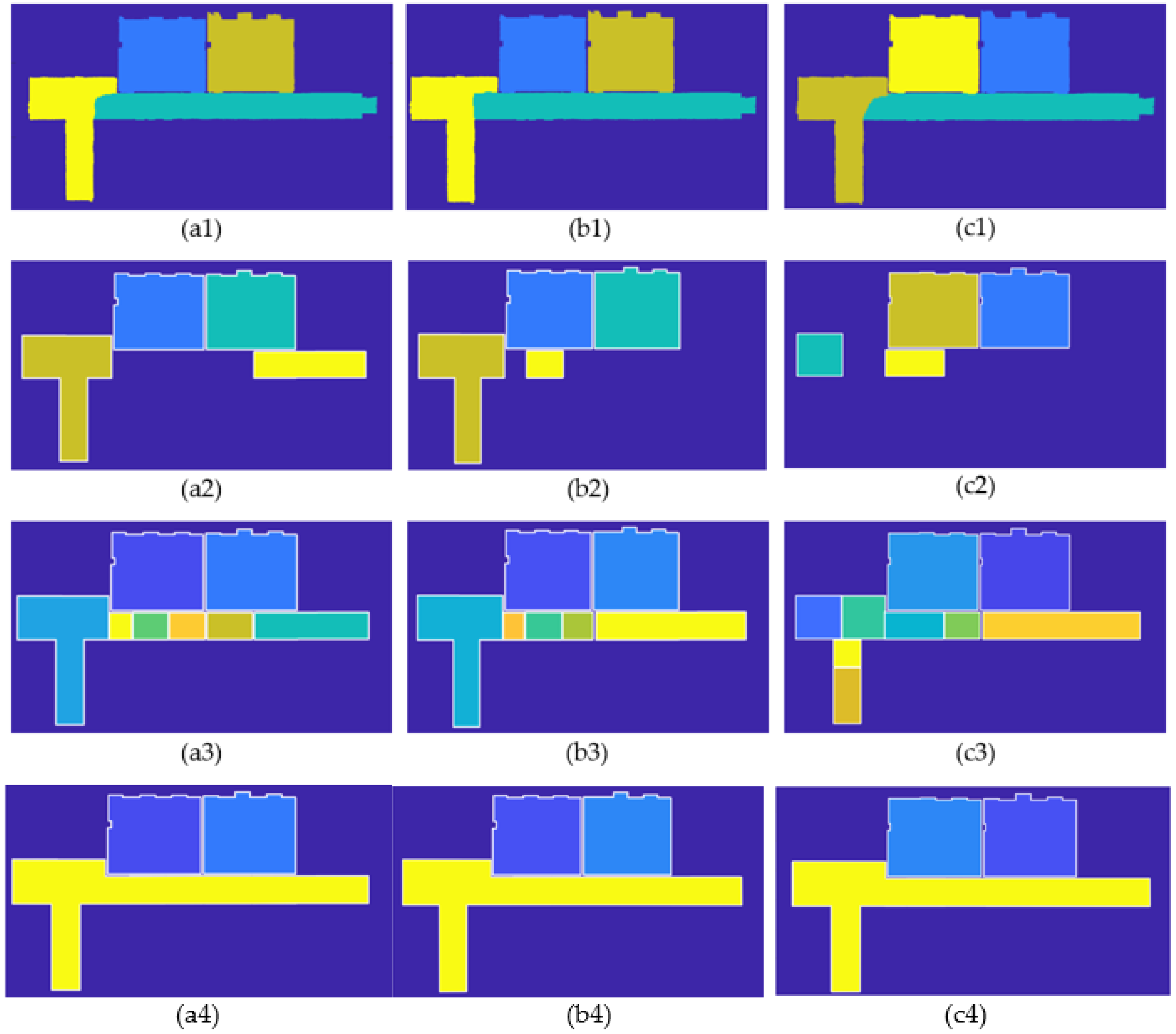
2.2.2. Segmentation of 2D Room Candidates (Step 2)

In Step 2, room segmentation was implemented as it can simplify the subsequent analyses and reduce the processing time [50]. Many existing room segmentation methods are based on visibility reasoning [48,55,58]. Although researchers have overcome the need to use the scanner location information, this often comes at the cost of computational complexity [59,60,61]. Since it is often easy to obtain scanner positions, such information was used in this study to simplify the room segmentation process.
The room segmentation in this study was formulated as a clustering problem, which was solved using a combination of the ray-casting and the k-medoids algorithms. Firstly, ray-casting was performed from each scanner location. By recording the paths that the ray can travel freely and the locations where it stops, the indoor space and the candidate locations of walls and openings can be obtained. After that, by projecting the ray-casting results onto a horizontal plane, an image representing the whole indoor area was obtained. The pixel size was set to 12 mm, which was the same as the voxel size used for the space voxelisation. The indoor area obtained was further refined by removing the pixels with distances (to the closest boundary of the indoor area along the X or Y axes) smaller than a threshold (e.g., 0.8 m used in this study). This was determined experimentally and was found to be effective in removing small erroneous local areas near the windows.
The image (representing 2D indoor area) obtained can be subsampled (e.g., at every 240 mm) along the X-axis and the Y-axis, respectively, for computational efficiency. The pixels in the subsampled image were clustered using the k-medoids algorithm [62].

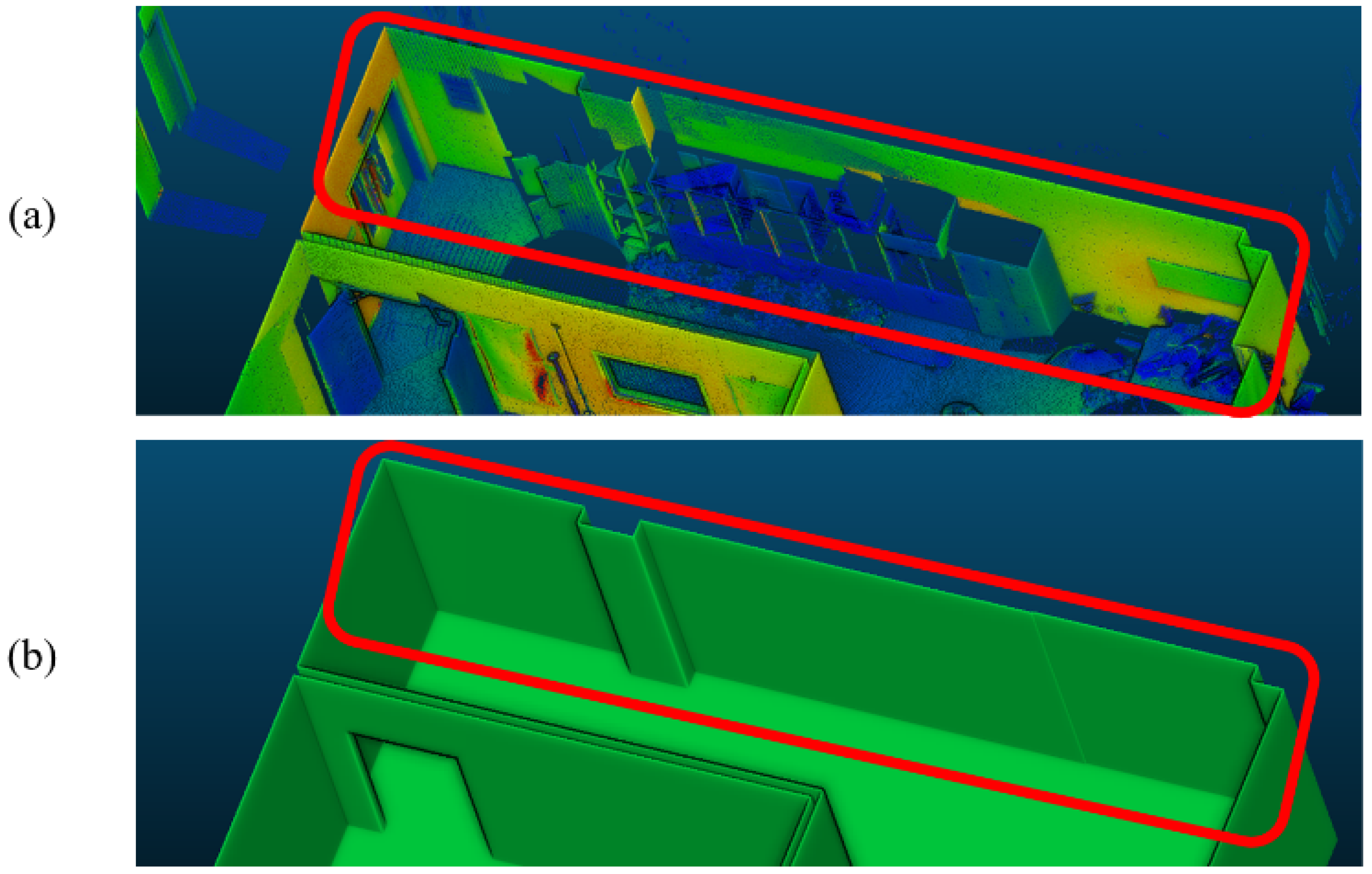
2.2.3. Three-Dimensional Reconstruction of Room Candidates (Step 3)

In the initial stage of the reconstruction, the initial boundary of each 2D room candidate was determined by continuously fitting rectangles of varying sizes to the corresponding local indoor areas. It should be noted that the grammar rules presented here are limited to the structures with orthogonal walls (i.e., the Manhattan world structure) as rectangles are used as the basic primitive. The boundary reconstruction grammar rules considered consist of the following steps:
  • For all rectangles, at least one edge is in contact with the boundary pixel of the segmented indoor area (Rule 1).
  • The first rectangle is fitted through the minimization process shown in Equation (1), which maximises the size of the first rectangle and keeps an aspect ratio of approximately 1. Based on this rule, it was found that the total number of subsequently filled rectangles needed to cover the entire indoor area can be significantly reduced, and thus the overall total processing time can be reduced.
    min Rule 1 = true ( max ( W ,   H ) + 0.0015 W H )
    where W is the width of the rectangle, and H is the height of the rectangle.
  • The newly fitted rectangles must touch but not intersect with the existing rectangles.
  • When no more rectangles can be fitted, the boundary of each 2D room candidate is determined using the Dijkstra algorithm (i.e., searching for the shortest path along the boundary of the fitted rectangles) [61].
Depending on the spatial confirmations of the rooms, the initial reconstruction may not guarantee the recognition of all the indoor space. To overcome this problem, the following set of criteria can be considered to determine if any remaining indoor areas can be added. If the uncovered indoor areas satisfy the following set of criteria, additional 2D boundaries are added to the existing ones using the boundary reconstruction grammar. This process can be run multiple times until the set of criteria are no longer valid.
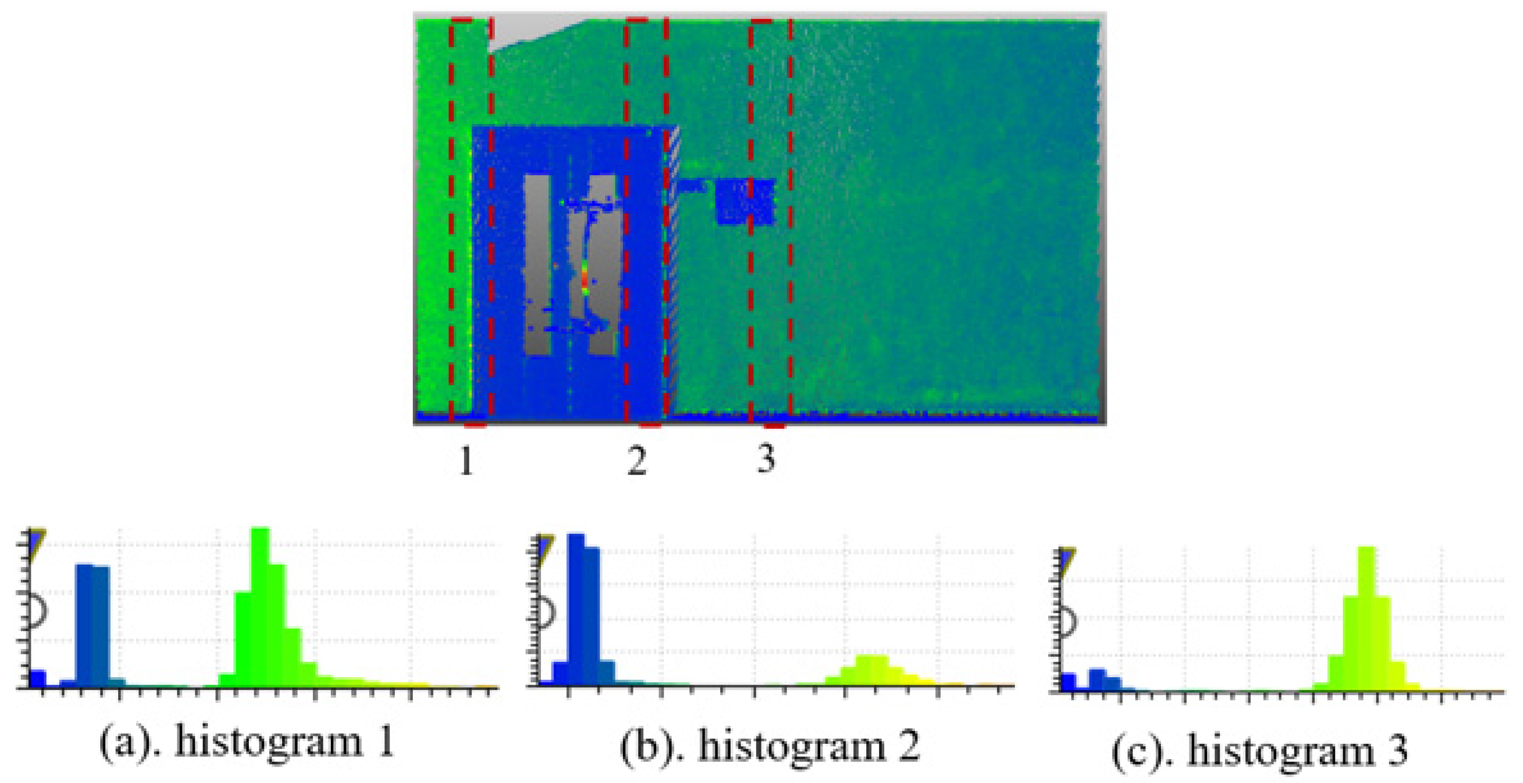
  • The sizes of the uncovered indoor areas are larger than 5% (determined by tests) of the average size of the reconstructed 2D boundaries. This rule is a quick filter for small independent areas.
  • The size of the largest rectangle within the uncovered indoor area is larger than 5% (determined by tests) of the average size of the reconstructed 2D boundaries. This rule is a more detailed filter for small independent areas.
  • The distance between the largest rectangle within the uncovered indoor area and the closest reconstructed boundary should be within 0.5 m.
  • The average point density within the uncovered indoor area is larger than 50% of the average point density in the reconstructed 2D boundaries.
For each 2D boundary, the floor to ceiling height was estimated using the horizontal planes fitted to the point cloud data representing floors and ceilings, respectively, by RANSAC. The 2D boundaries were extruded to the estimated room height(s) to form the 3D geometric models of the room candidates.

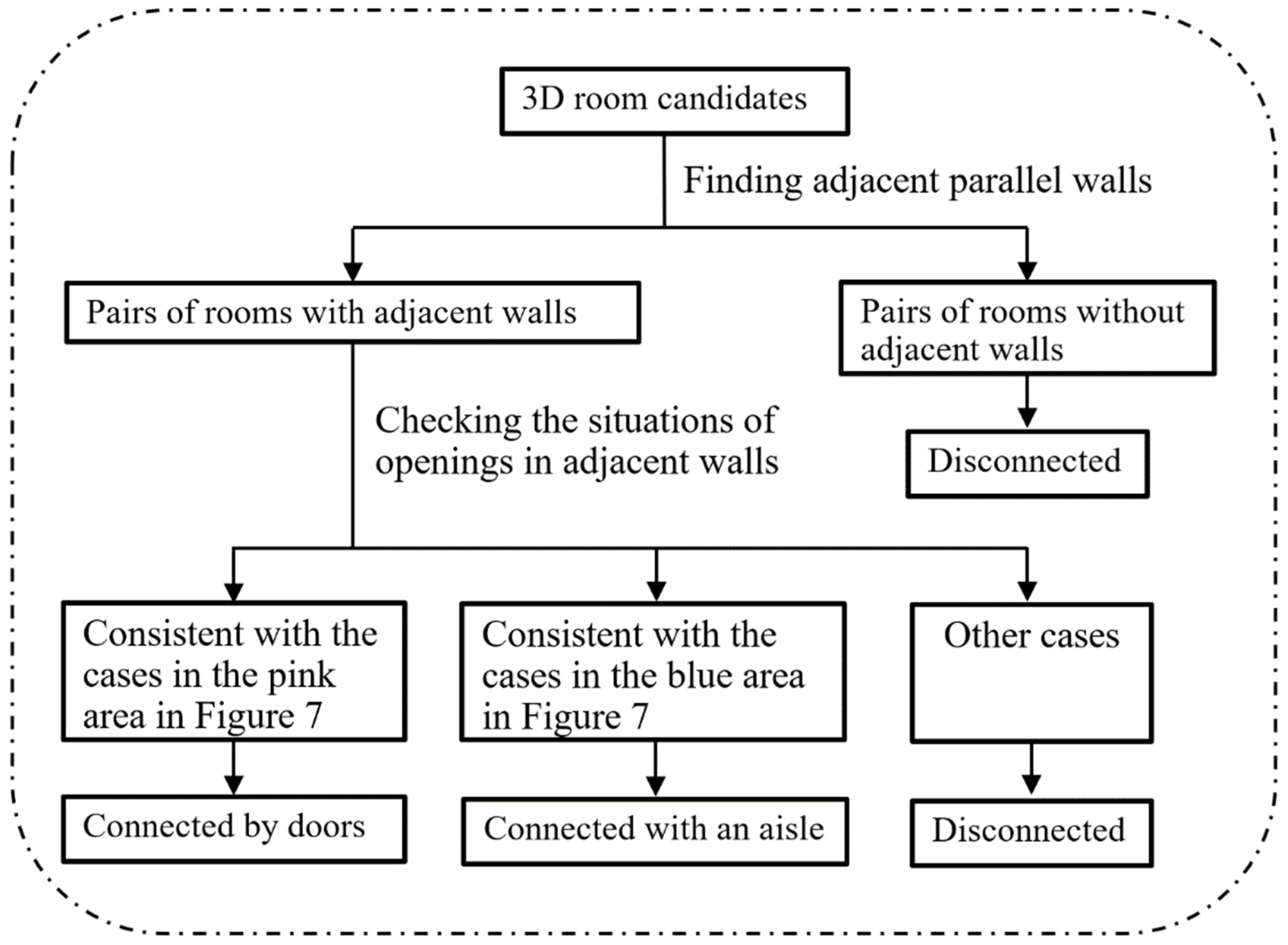
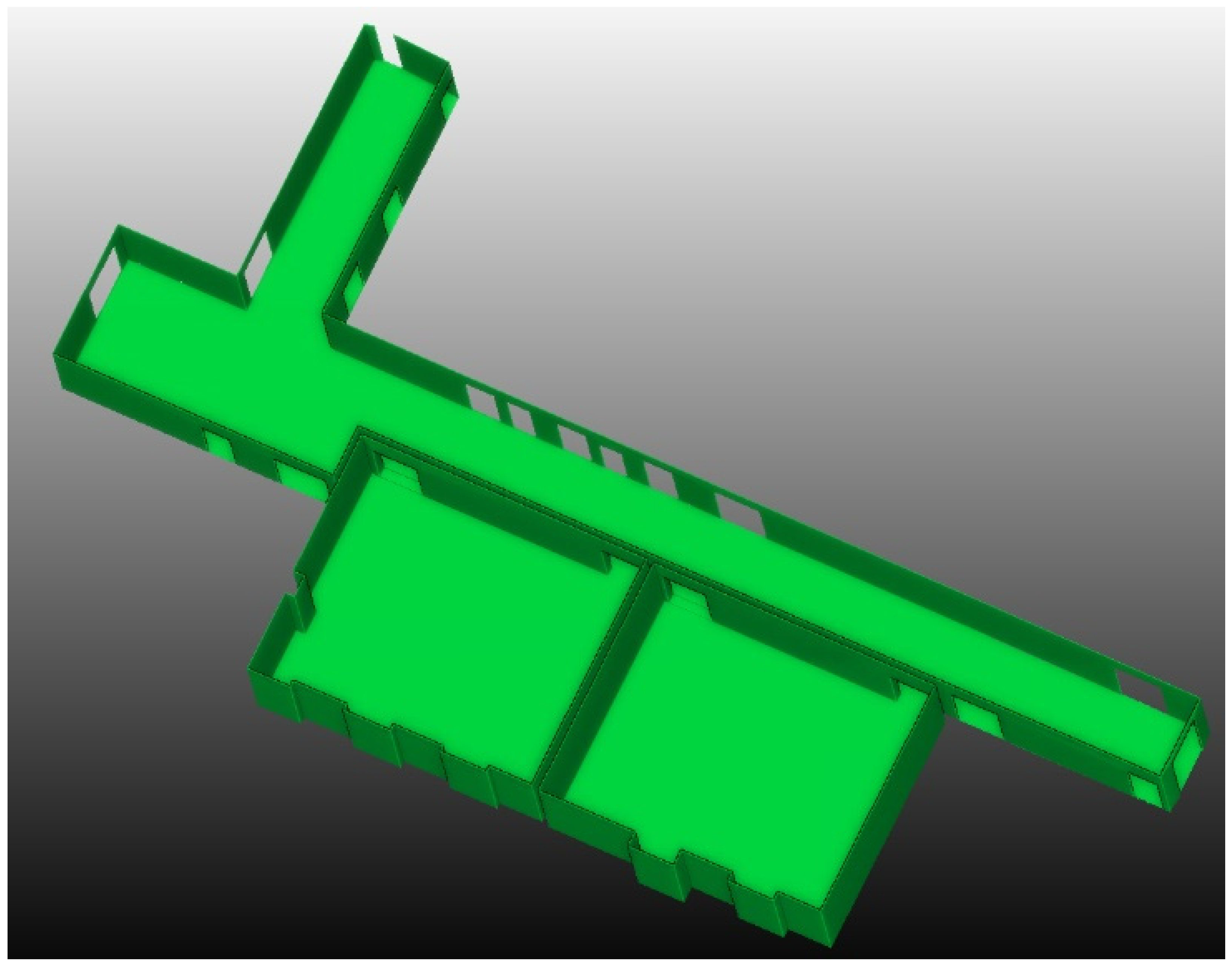
2.2.4. Connection Analysis for 3D Room Candidates (Step 4)

To correctly construct the final building model, it is essential to analyse the connections between the 3D room candidates obtained in Step 3. The grammar rules considered for the connection analysis are straightforward and are based on the observation of typical connections between rooms. There are mainly three types of connection relations between 3D room candidates: connected by a door, connected by an aisle (belonging to the same room) or disconnected. According to the relative locations and the sizes of the openings (obtained using the ray-casting in the room segmentation stage) on two adjacent walls (parallel and within a distance of 1.0 m), the connection types between adjacent 3D room candidates can be determined using the following room-connection grammar, and the corresponding procedure is summarised in Figure 6:
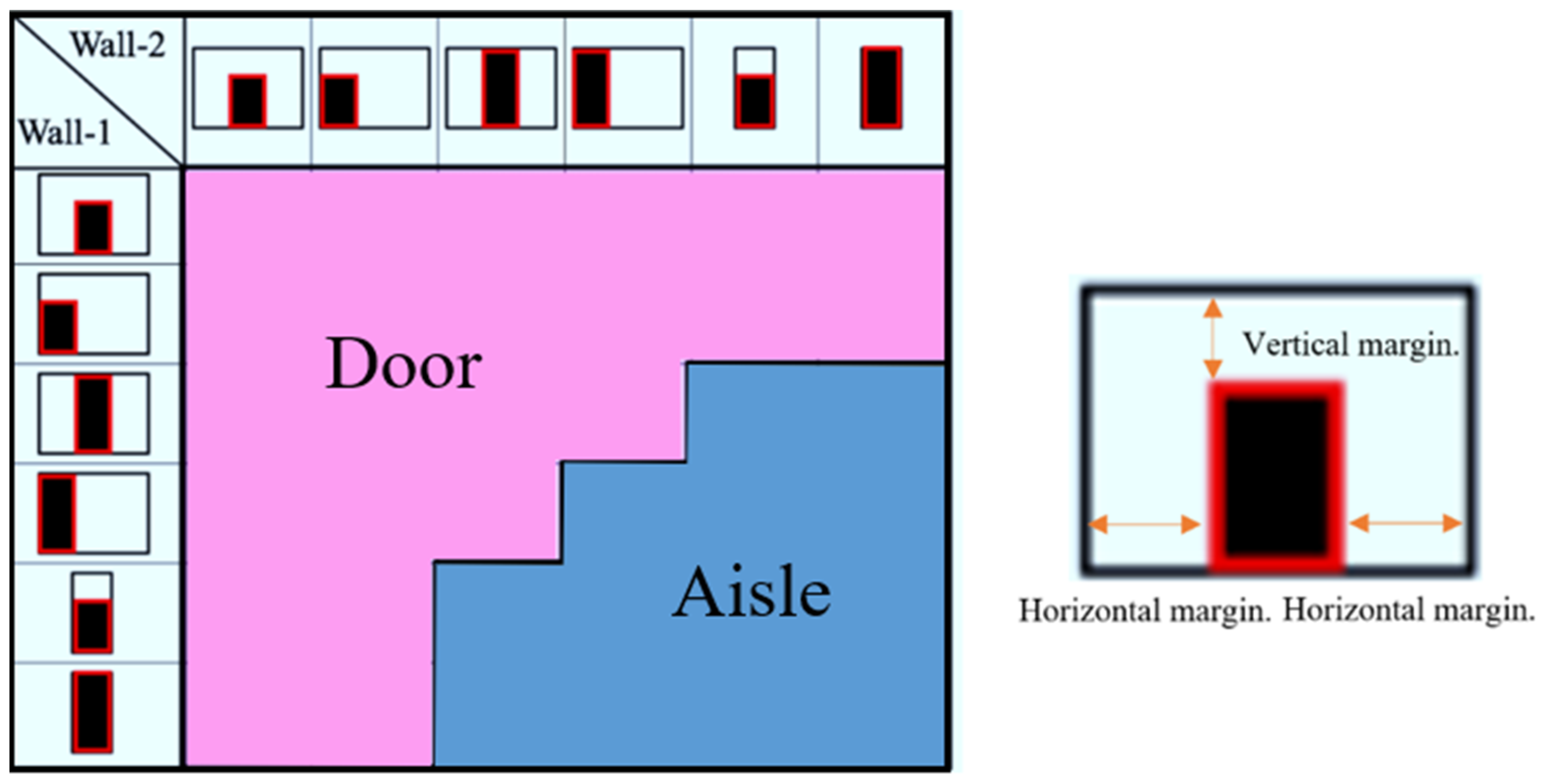
  • If there is no opening on two adjacent walls or the openings do not fall into one of the situations shown in Figure 7, they are labelled as disconnected.
  • The adjacent 3D room candidates are merged if they are connected by an aisle.
  • Otherwise, doors are constructed at the openings between the 3D room candidates.
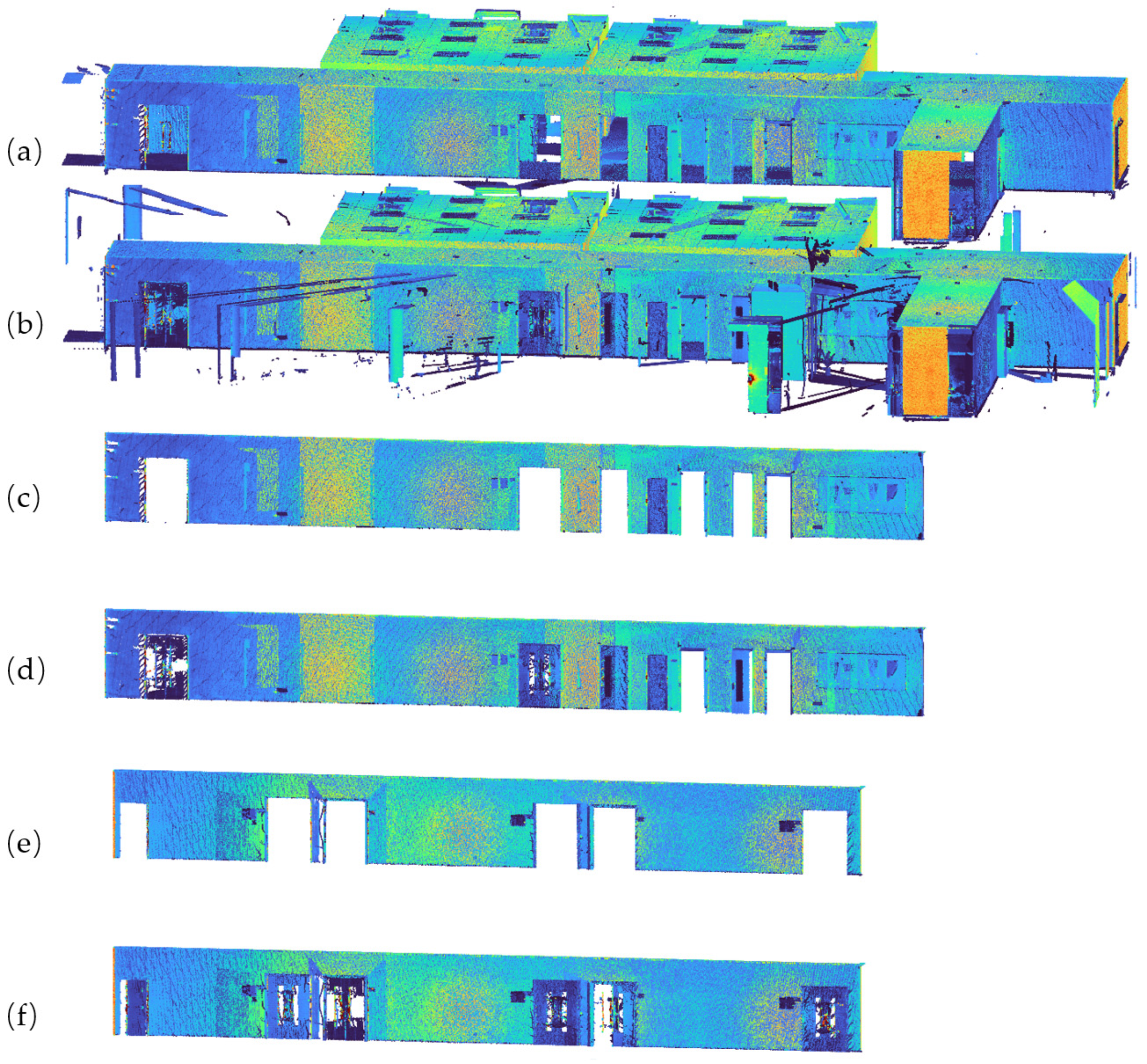
By assuming the bottom edge of a door was connected to the floor, three margins (two horizontal margins and one vertical margin, as shown in Figure 7) between an opening and the nearest wall boundary were used to classify the room connections. Based on the observations on the doors, the thresholds for the horizontal and the vertical margins were set to be 0.1 m and 0.05 times the wall height, respectively. Based on the configurations of margins, the potential door openings can be divided into six different situations shown in the first row or column of the classification in Figure 7. By checking if the openings on the adjacent walls were located at almost the same position and fell into one of the aforementioned six situations, the type of room connection can be determined. Following the room connection analysis, the topological relations between the rooms were obtained and used for generating the final geometric models, which are presented in Section 3.

3. Results

The steps elaborated in Section 2 were realised using the codes developed in MATLAB, which run in a computer with Windows 10 (64-bit) system, an AMD 3950x processor and 64G DDR4 RAM. The same grammar rules and the same values of the corresponding parameters were applied to all the sites considered. For ease of demonstration, Site 1 was used as an example to present the output(s) of each step.
Figure 8a shows the point cloud data where the data points representing the doors were successfully filtered out. To better visualise the results, two walls with the door removed are shown separately in Figure 8c,e. For a comparison, the corresponding original point cloud data are also shown in Figure 8b,d,f.
The final 2D indoor area obtained using the ray-casting analysis is shown in Figure 9, where the dark blue colour represents the outdoor region, black dots represent the scanner locations, and the yellow lines represent the ray paths.
Based on the 2D indoor area in Figure 9, if the connection line of any two pixels did not pass through the outdoor area, the Euclidean distance between them was calculated. Otherwise, the distance between two pixels was taken as the Euclidean distance plus the square of the detour distance. Using 100 initial seeding pixels selected from the indoor area, the k-medoids algorithm was repeated for the cluster merging until the distances between adjacent clusters were larger than 0.5 m, leading to a segmented image using the subsampled pixels. The segmentation results were extended to all the pixels of the original image (i.e., without subsampling) according to the class of the nearest subsample pixel. The whole process was repeated for three rounds to see the likely variations in the outputs. Figure 10a1,b1,c1 show the final segmented image for the three rounds, respectively, where the 2D room candidates are labelled in different colours.
Using the reconstruction grammar rules defined in Section 2.2.3, the initial 2D boundaries obtained from each room candidate are shown in Figure 10a2,b2,c2 for the three rounds of realisations, respectively. It is observed that the boundaries created did not cover the full footprint of the indoor area (more specifically, some corridor areas were missing). Additionally, the output of each realisation also varies due to the fitting of random rectangles to each individual segmented room candidate.
Following the criteria for identifying any remaining indoor area, the reconstruction grammar rules were applied, leading to the outputs shown in Figure 10a3,b3,c3 for the three rounds. It can be observed that almost all the indoor areas have successfully been covered. It was also found that the reconstruction rules were applied only once to obtain those satisfactory results, although this process can be repeated multiple times. Regardless of the variations in the room candidates shown in Figure 10a3,b3,c3, the final boundaries obtained for the three rounds after the connection analyses (Section 2.2.4) were found to be almost the same, as illustrated in Figure 10a4,b4,c4.
The final watertight 3D model for each site was compiled and shown in Figure 11. It was found that the approach proposed correctly reconstructed all the rooms and the main structural elements (doors, walls, floors, ceilings, and columns) for the study sites considered. The key performance metrics of the proposed approach on the study sites are summarised in Table 1.
The distances between individual data points representing the structural elements and the corresponding nearest planes of the geometric model (in Figure 11) generated for each site were calculated, the average value of which was used as the error statistics to assess the overall accuracy of the final 3D geometric model created. The mean errors (given in Table 1) for the six sites considered were found to be 13–21 mm, in comparison to 8–54 mm (Table 2) reported in similar studies in the literature [19,21,22,23,24]. It should be noted that the mean errors are not only affected by the reconstruction method itself but also depend on several other factors, such as the measurement accuracy of the devices used to collect the data and the presence of thin objects (e.g., whiteboard at Site 2) attached to the wall and/or ceiling surfaces.
Furthermore, the grammar-based approach proposed was found to be robust for indoor environments with high occlusions. For example, both the column and the wall surfaces were reconstructed correctly for the occluded parts of Site 3, as shown in Figure 12.
The processing time for creating the final integrated watertight model using the approach proposed was less than 5 min for an extremely high density dataset of Site 2 (approximately 469 million data points). It is generally more efficient than many methods in the literature where the processing time ranged from several minutes to hours for point cloud data of much smaller densities [11,20,22,23,24]. Table 3 shows a comparison of computational efficiency with some existing methods in the literature. Since those methods were typically tested with point cloud data from multiple sites of varying complexities, only the case with the maximum processing time taken from each study is shown in Table 3. In addition, the total computational time reported for the sites considered in this study also includes that taken for the filtering of the door information, which was not part of the tasks in other studies shown in Table 3.
For a watertight model, the doors on the exterior walls are neglected using the grammar rules given in Section 2.2.3. As such, no doors on the exterior boundary of the models in Figure 11 were shown. However, those grammar rules can be slightly modified to enable the detection of the doors on all walls, including those on the exterior boundaries. The modified rules are:
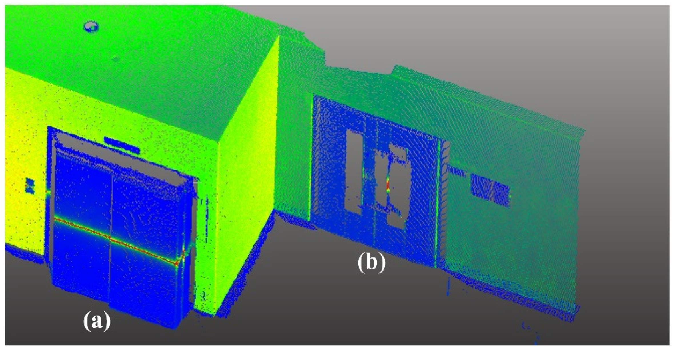
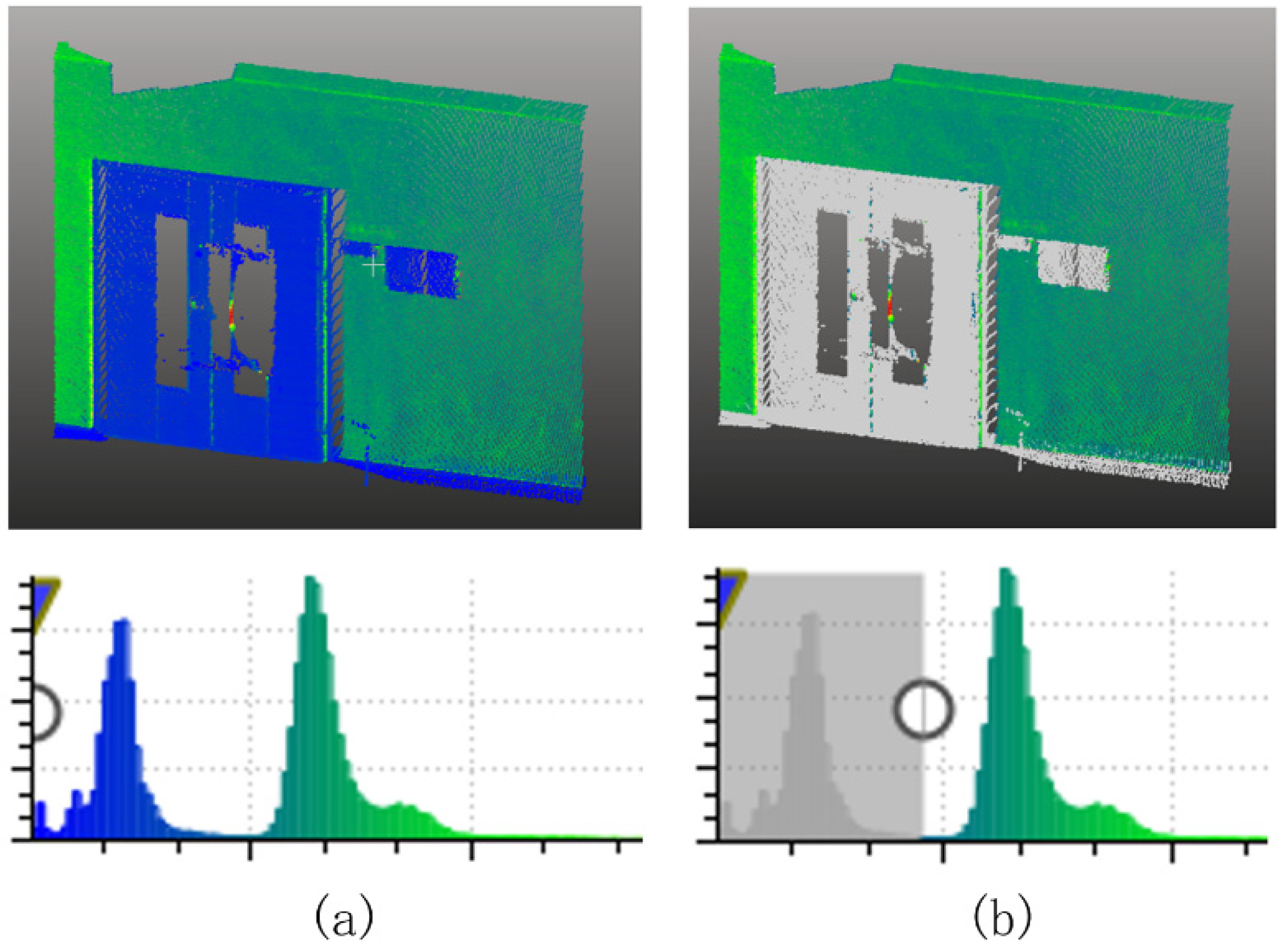
  • The thresholds of the wall opening are 0.6 m (width) by 1.8 m (height) since most doors have larger sizes than this.
  • At least one margin between the opening and its nearest wall boundary is larger than the corresponding margin threshold mentioned in Section 2.2.3.
To demonstrate this, the modified grammar rules were applied to the data of Site 1. Figure 13 shows all the doors modelled, including those on the exterior boundaries. An in situ observation of Site 1 confirms that all the doors were correctly detected and included in the model.

4. Conclusions

In this article, an efficient approach was introduced for the automatic generation of 3D watertight geometries of the Manhattan world structures. While achieving similar modelling accuracy compared to other existing methods, our method can handle much denser point clouds (e.g., tens of times denser point clouds) in less time. This approach can be used to construct an accurate watertight building model with segmented rooms and doors, which is of use in energy simulations of buildings. The approach also provides an effective means of extracting the topological relations between rooms, which are essential for path planning and navigation. Furthermore, it was demonstrated that the approach was effective even when there are occlusions in the point cloud data. Future research work may be focused on the extension of the grammar rules to non-Manhattan world structures.

Author Contributions

Conceptualization, Y.C. and L.F.; methodology, Y.C. and L.F.; software, Y.C.; validation, Y.C. and L.F.; formal analysis, Y.C.; investigation, Y.C.; resources, Y.C.; data curation, Y.C.; writing—original draft preparation, Y.C. and L.F.; writing—review and editing, Y.C. and L.F.; visualization, Y.C.; supervision, L.F.; project administration, L.F.; funding acquisition, L.F. All authors have read and agreed to the published version of the manuscript.

Funding

This research was funded by XJTLU Key Program Special Fund, grant number KSF-E-40, XJTLU Research Development Fund, grant number RDF-18-01-40, and Natural Science Foundation of Jiangsu Province, grant number BK20160393.

Institutional Review Board Statement

Not applicable.

Informed Consent Statement

Not applicable.

Data Availability Statement

The data presented in this study are available on request from the corresponding author. The point cloud data are not publicly available because it was collected within private property and subjected to privacy issues.

Conflicts of Interest

The authors declare no conflict of interest.

References

  1. EUR-Lex-31993L0076. Council Directive 93/76/EEC of 13 September 1993 to Limit Carbon Dioxide Emissions by Improving Energy Efficiency (SAVE). Available online: https://eur-lex.europa.eu/legal-content/EN/ALL/?uri=CELEX%3A31993L0076 (accessed on 1 April 2021).
  2. EUR-Lex-02012L0027-20200101. Directive 2012/27/EU of the European Parliament and of the Council of 25 October 2012 on Energy Efficiency. Available online: https://eur-lex.europa.eu/legal-content/EN/TXT/?uri=CELEX:02012L0027-20200101 (accessed on 1 April 2021).
  3. IDEA. Plan Nacional Integrado de Energía y Clima (PNIEC) 2021–2030. Available online: https://www.idae.es/informacion-y-publicaciones/plan-nacional-integrado-de-energia-y-clima-pniec-2021-2030 (accessed on 1 April 2021).
  4. Becerik-Gerber, B.; Jazizadeh, F.; Li, N.; Calis, G. Application areas and data requirements for BIM-enabled facilities management. J. Constr. Eng. Manag. 2012, 138, 431–442. [Google Scholar] [CrossRef]
  5. Westoby, M.J.; Brasington, J.; Glasser, N.F.; Hambrey, M.J.; Reynolds, J.M. “Structure-from-Motion” photogrammetry: A low-cost, effective tool for geoscience applications. Geomorphology 2012, 179, 300–314. [Google Scholar] [CrossRef] [Green Version]
  6. Drury, B.; Curtis, O.; Linda, K.; Frederick, C. EnergyPlus: Energy simulation program. ASHRAE J. 2000, 42, 49–56. [Google Scholar]
  7. Diakité, A.A.; Zlatanova, S. Spatial subdivision of complex indoor environments for 3D indoor navigation. Int. J. Geogr. Inf. Sci. 2018, 32, 213–235. [Google Scholar] [CrossRef] [Green Version]
  8. Montilla, Y.M.; León-Sánchez, C. 3D modelling of a building oriented to indoor navigation system for users with different mobility conditions. ISPRS Ann. Photogramm. Remote Sens. Spat. Inf. Sci. 2020, VI-4/W2-2020, 103–109. [Google Scholar] [CrossRef]
  9. Zhang, C.; Ong, L. Sensitivity analysis of building envelop elements impact on energy consumptions using BIM. Open J. Civ. Eng. 2017, 7, 488–508. [Google Scholar] [CrossRef] [Green Version]
  10. Nizam, R.S.; Zhang, C.; Tian, L. A BIM based tool for assessing embodied energy for buildings. Energy Build. 2018, 170, 1–14. [Google Scholar] [CrossRef]
  11. Nikoohemat, S.; Diakité, A.A.; Zlatanova, S.; Vosselman, G. Indoor 3D reconstruction from point clouds for optimal routing in complex buildings to support disaster management. Autom. Constr. 2020, 113, 103109. [Google Scholar] [CrossRef]
  12. Akcamete, A.; Akinci, B.; Garrett, J.H., Jr. Potential utilization of building information models for planning maintenance activities. In Proceedings of the 17th International Workshop on Intelligent Computing in Civil and Building Engineering, Tampere, Finland, 5–7 July 2018. [Google Scholar]
  13. Valinejadshoubi, M.; Bagchi, A.; Moselhi, O. Development of a BIM-based data management system for structural health monitoring with application to modular buildings: Case study. J. Comput. Civ. Eng. 2019, 33, 5019003. [Google Scholar] [CrossRef]
  14. O’Shea, M.; Murphy, J. Design of a BIM integrated structural health monitoring system for a historic offshore lighthouse. Buildings 2020, 10, 131. [Google Scholar] [CrossRef]
  15. Zou, Y.; Kiviniemi, A.; Jones, S.W. A review of risk management through BIM and BIM-related technologies. Saf. Sci. 2017, 97, 88–98. [Google Scholar] [CrossRef]
  16. Enshassi, M.S.A.; Walbridge, S.; West, J.S.; Haas, C.T. Integrated risk management framework for tolerance-based mitigation strategy decision support in modular construction projects. J. Manag. Eng. 2019, 35, 5019004. [Google Scholar] [CrossRef]
  17. Chen, K.; Lu, W. Bridging BIM and building (BBB) for information management in construction: The underlying mechanism and implementation. Eng. Constr. Archit. Manag. 2019, 26, 1518–1532. [Google Scholar] [CrossRef]
  18. Darko, A.; Chan, A.P.C.; Yang, Y.; Tetteh, M.O. Building information modeling (BIM)-based modular integrated construction risk management—Critical survey and future needs. Comput. Ind. 2020, 123, 103327. [Google Scholar] [CrossRef]
  19. Adan, A.; Huber, D. 3D reconstruction of interior wall surfaces under occlusion and clutter. In Proceedings of the International Conference on 3D Imaging, Modeling, Processing, Visualization and Transmission, Zurich, Switzerland, 13–15 October 2012. [Google Scholar]
  20. Sanchez, V.; Zakhor, A. Planar 3D modeling of building interiors from point cloud data. In Proceedings of the International Conference on Image Processing, ICIP, Orlando, FL, USA, 30 September–3 October 2012. [Google Scholar]
  21. Wang, R.; Xie, L.; Chen, D. Modeling indoor spaces using decomposition and reconstruction of structural elements. Photogramm. Eng. Remote Sensing 2017, 83, 827–841. [Google Scholar] [CrossRef]
  22. Tran, H.; Khoshelham, K.; Kealy, A.; Díaz-Vilariño, L. Shape grammar approach to 3D modeling of indoor environments using point clouds. J. Comput. Civ. Eng. 2019, 33, 4018055. [Google Scholar] [CrossRef]
  23. Ochmann, S.; Vock, R.; Klein, R. Automatic reconstruction of fully volumetric 3D building models from oriented point clouds. ISPRS J. Photogramm. Remote Sens. 2019, 151, 251–262. [Google Scholar] [CrossRef] [Green Version]
  24. Sanchez, J.; Denis, F.; Dupont, F.; Trassoudaine, L.; Checchin, P. Data-driven modeling of building interiors from lidar point clouds. ISPRS Ann. Photogramm. Remote Sens. Spat. Inf. Sci. 2020, V-2-2020, 395–402. [Google Scholar] [CrossRef]
  25. Nurunnabi, A.; Belton, D.; West, G. Diagnostic-robust statistical analysis for local surface fitting in 3D point cloud data. ISPRS Ann. Photogramm. Remote Sens. Spat. Inf. Sci. 2012, 1, 269–274. [Google Scholar] [CrossRef] [Green Version]
  26. Schnabel, R.; Wahl, R.; Klein, R. Efficient RANSAC for point-cloud shape detection. Comput. Graph. Forum 2007, 26, 214–226. [Google Scholar] [CrossRef]
  27. Budroni, A.; Boehm, J. Automated 3D reconstruction of interiors from point clouds. Int. J. Archit. Comput. 2010, 8, 55–73. [Google Scholar] [CrossRef]
  28. Barnea, S.; Filin, S. Segmentation of terrestrial laser scanning data using geometry and image information. ISPRS J. Photogramm. Remote Sens. 2013, 76, 33–48. [Google Scholar] [CrossRef]
  29. Torr, P.H.S.; Zisserman, A. MLESAC: A new robust estimator with application to estimating image geometry. Comput. Vis. Image Underst. 2000, 78, 138–156. [Google Scholar] [CrossRef] [Green Version]
  30. Rusu, R.B.; Marton, Z.C.; Blodow, N.; Holzbach, A.; Beetz, M. Model-based and learned semantic object labeling in 3D point cloud maps of kitchen environments. In Proceedings of the IEEE/RSJ International Conference on Intelligent Robots and Systems, St. Louis, MO, USA, 10–15 October 2009. [Google Scholar]
  31. Pu, S.; Vosselman, G. Automatic extraction of building features from terrestrial laser scanning. ISPRS Ann. Photogramm. Remote Sens. Spat. Inf. Sci. 2006, 36, 25–27. [Google Scholar]
  32. Previtali, M.; Scaioni, M.; Barazzetti, L.; Brumana, R. A flexible methodology for outdoor/indoor building reconstruction from occluded point clouds. ISPRS Ann. Photogramm. Remote Sens. Spat. Inf. Sci. 2014, II-3, 119–126. [Google Scholar] [CrossRef] [Green Version]
  33. Thomson, C.; Boehm, J. Automatic geometry generation from point clouds for BIM. Remote Sens. 2015, 7, 11753–11775. [Google Scholar] [CrossRef] [Green Version]
  34. Tran, H.; Khoshelham, K. A stochastic approach to automated reconstruction of 3D models of interior spaces from point clouds. ISPRS Ann. Photogramm. Remote Sens. Spat. Inf. Sci. 2019, IV-2/W5, 299–306. [Google Scholar] [CrossRef] [Green Version]
  35. Díaz-Vilariño, L.; Khoshelham, K.; Martínez-Sánchez, J.; Arias, P. 3D modeling of building indoor spaces and closed doors from imagery and point clouds. Sensors 2015, 15, 3491–3512. [Google Scholar] [CrossRef] [Green Version]
  36. Hong, S.; Jung, J.; Kim, S.; Cho, H.; Lee, J.; Heo, J. Semi-automated approach to indoor mapping for 3D as-built building information modeling. Comput. Environ. Urban Syst. 2015, 51, 34–46. [Google Scholar] [CrossRef]
  37. Xiong, X.; Adan, A.; Akinci, B.; Huber, D. Automatic creation of semantically rich 3D building models from laser scanner data. Autom. Constr. 2013, 31, 325–337. [Google Scholar] [CrossRef] [Green Version]
  38. Gröger, G.; Plümer, L. Derivation of 3D indoor models by grammars for route planning. Photogramm. Fernerkundung Geoinf. 2010, 2010, 191–206. [Google Scholar] [CrossRef]
  39. Khoshelham, K.; Díaz-Vilariño, L. 3D modelling of interior spaces: Learning the language of indoor architecture. ISPRS Ann. Photogramm. Remote Sens. Spat. Inf. Sci. 2014, XL-5, 321–326. [Google Scholar] [CrossRef] [Green Version]
  40. Becker, S. Generation and application of rules for quality dependent façade reconstruction. ISPRS J. Photogramm. Remote Sens. 2009, 64, 640–653. [Google Scholar] [CrossRef]
  41. Müller, P.; Wonka, P.; Haegler, S.; Ulmer, A.; van Gool, L. Procedural modeling of buildings. In Proceedings of the ACM SIGGRAPH 2006 Papers, SIGGRAPH ’06, Boston, MA, USA, 30 July–3 August 2006. [Google Scholar]
  42. Wonka, P.; Wimmer, M.; Sillion, F.; Ribarsky, W. Instant architecture. In Proceedings of the ACM SIGGRAPH 2003 Papers, SIGGRAPH ’03, San Diego, CA, USA, 27–31 July 2003. [Google Scholar]
  43. Becker, S.; Peter, M.; Fritsch, D. Grammar-supported 3D indoor reconstruction from point clouds for “as-Built” BIM. ISPRS Ann. Photogramm. Remote Sens. Spat. Inf. Sci. 2015, II-3/W4, 301–302. [Google Scholar] [CrossRef] [Green Version]
  44. Marvie, J.E.; Perret, J.; Bouatouch, K. The FL-system: A functional L-system for procedural geometric modeling. Vis. Comput. 2005, 21, 329–339. [Google Scholar] [CrossRef]
  45. Sanabria, S.L.; Mitchell, W.J. The logic of architecture: Design, computation, and cognition. Technol. Cult. 1992, 33, 625. [Google Scholar] [CrossRef]
  46. Bassier, M.; Yousefzadeh, M.; Vergauwen, M. Comparison of 2d and 3d wall reconstruction algorithms from point cloud data for as-built bim. J. Inf. Technol. Constr. 2020, 25, 173–192. [Google Scholar] [CrossRef]
  47. Macher, H.; Landes, T.; Grussenmeyer, P. From point clouds to building information models: 3D semi-automatic reconstruction of indoors of existing buildings. Appl. Sci. 2017, 7, 1030. [Google Scholar] [CrossRef] [Green Version]
  48. Turner, E.; Zakhor, A. Watertight planar surface meshing of indoor point-clouds with voxel carving. In Proceedings of the International Conference on 3D Vision, 3DV 2013, Seattle, WA, USA, 29 June–1 July 2013. [Google Scholar]
  49. Parish, Y.I.H.; Müller, P. Procedural modeling of cities. In Proceedings of the 28th Annual Conference on Computer Graphics and Interactive Techniques, SIGGRAPH 2001, Los Angeles, CA, USA, 12–17 August 2001. [Google Scholar]
  50. Kelly, G.; McCabe, H. A survey of procedural techniques for city generation. ITB J. 2006, 7, 342–351. [Google Scholar] [CrossRef]
  51. Stiny, G.; Gips, J. Shape grammars and the generative specification of painting and sculpture. In Proceedings of the Information Processing, IFIP Congress 1971, Volume 2, Ljubljana, Slovenia, 23–28 August 1971. [Google Scholar]
  52. Boulch, A.; Houllier, S.; Marlet, R.; Tournaire, O. Semantizing complex 3D scenes using constrained attribute grammars. Eurograph. Symp. Geom. Process. 2013, 32, 33–34. [Google Scholar] [CrossRef]
  53. Dick, A.R.; Torr, P.H.S.; Cipolla, R. Modelling and interpretation of architecture from several images. Int. J. Comput. Vis. 2004, 60, 111–134. [Google Scholar] [CrossRef] [Green Version]
  54. Bassier, M.; Vergauwen, M. Topology reconstruction of BIM wall objects from point cloud data. Remote Sens. 2020, 12, 1800. [Google Scholar] [CrossRef]
  55. Oesau, S.; Lafarge, F.; Alliez, P. Indoor scene reconstruction using feature sensitive primitive extraction and graph-cut. ISPRS J. Photogramm. Remote Sens. 2014, 90, 68–82. [Google Scholar] [CrossRef] [Green Version]
  56. Turner, E.; Zakhor, A. Multistory floor plan generation and room labeling of building interiors from laser range data. In Communications in Computer and Information Science; Springer: Berlin/Heidelberg, Germany, 2015; Volume 550. [Google Scholar]
  57. CBRE Build. Available online: https://www.cbrebuild.com/ (accessed on 5 January 2021).
  58. Ochmann, S.; Vock, R.; Wessel, R.; Klein, R. Automatic reconstruction of parametric building models from indoor point clouds. Comput. Graph. 2016, 54, 94–103. [Google Scholar] [CrossRef] [Green Version]
  59. Ambrus, R.; Claici, S.; Wendt, A. Automatic room segmentation from unstructured 3-D data of indoor environments. IEEE Robot. Autom. Lett. 2017, 2, 749–756. [Google Scholar] [CrossRef]
  60. Turner, E.; Zakhor, A. Floor plan generation and room labeling of indoor environments from: Laser range data. In Proceedings of the 9th International Conference on Computer Graphics Theory and Applications, Lisbon, Portugal, 5–8 January 2014. [Google Scholar]
  61. Dijkstra, E.W. A note on two problems in connexion with graphs. Numer. Math. 1959, 1, 269–271. [Google Scholar] [CrossRef] [Green Version]
  62. Park, H.S.; Jun, C.H. A simple and fast algorithm for K-medoids clustering. Expert Syst. Appl. 2009, 36, 3336–3341. [Google Scholar] [CrossRef]
Figure 1. Registered point cloud data of six sites: (a) Site 1, (b) Site 2, (c) Site 3, (d) Site 4, (e) Site 5, (f) Site 6.
Remotesensing 13 01947 g001
Figure 2. Flowchart of the approach proposed: Pre-process, segmentation of 2D room candidates, reconstruction for 3D room candidates, connection analysis of 3D room candidates and final model compilation.
Remotesensing 13 01947 g002
Figure 3. Two types of doors: (a) non-coplanar doors, (b) coplanar doors.
Remotesensing 13 01947 g003
Figure 4. Removal of data points representing coplanar doors: (a) the intensity histogram for a region with a coplanar door, (b) filtering out the points in the lower peak of the intensity histogram.
Remotesensing 13 01947 g004
Figure 5. Intensity histograms at three different locations of the moving window: (a) histogram 1, (b) histogram 2, (c) histogram 3.
Remotesensing 13 01947 g005
Figure 6. Flowchart for the room connection analysis.
Remotesensing 13 01947 g006
Figure 7. Initial and additional boundaries of the 2D room candidates.
Remotesensing 13 01947 g007
Figure 8. The detection and removal of the door information: the point cloud data with the doors removed (a,c,e) and the original point cloud data (b,d,f).
Remotesensing 13 01947 g008
Figure 9. Refined 2D projection of the ray-casting results (i.e., 2D indoor area).
Remotesensing 13 01947 g009
Figure 10. Three rounds (i.e., a, b, c) of the realisations of the grammar rules: (a1,b1,c1) represent the segmented 2D indoor areas (i.e., room candidates) in each round, (a2,b2,c2) represent the initial boundaries of the 2D room candidates in each round, (a3,b3,c3) represent initial and additional boundaries of the 2D room candidates in each round, (a4,b4,c4) represent the final boundary after the connection analysis in each round.
Remotesensing 13 01947 g010
Figure 11. The point clouds and the corresponding watertight models (ceilings were removed for better visualisation) for the six sites: (a) Site 1, (b) Site 2, (c) Site 3, (d) Site 4, (e) Site 5, (f) Site 6.
Remotesensing 13 01947 g011
Figure 12. (a) Surfaces with occlusions in Site 3, (b) the corresponding model constructed.
Remotesensing 13 01947 g012
Figure 13. Three-dimensional geometric model of Site 1 with all the doors being successfully modelled (ceilings were removed for better visualisation).
Remotesensing 13 01947 g013
Table 1. The key performance metrics of the proposed approach.
Performance MetricsSite 1Site 2Site 3Site 4Site 5Site 6
Number of input points476,417,203469,140,41140,143,4124,933,1724,534,1364,227,235
Run time (s)237284131107122149
Mean point-to-model error (mm)131813211916
Max point-to-model error (mm)212920272725
The detection rate of doors (%)100100100100100100
The detection rate of rooms (%)100100100100100100
Table 2. Comparison of the mean point-to-model error between our approach and other methods.
ApproachesNumber of Data Points (Million)Mean Point-to-Model Error (mm)
[19]. 201150054
[21]. 20170.8–214–35
[22]. 20190.3–3.013–33
[24]. 20202.58
Our approach4.2–476.413–21
Table 3. Comparison of the most time-consuming cases between our approach and other methods.
Ref. YearNumber of Data Points (Million)Process Time (s)
[20]. 20126.712,798
[23]. 201934.9710
[11]. 20207.4648
[22]. 20190.3105
[24]. 20202.5300
Our approach (Site 2)469.1284
Publisher’s Note: MDPI stays neutral with regard to jurisdictional claims in published maps and institutional affiliations.

