
Short-Term Wind Power Forecasting at the Wind Farm Scale Using Long-Range Doppler LiDAR


Abstract
1. Introduction
2. Background
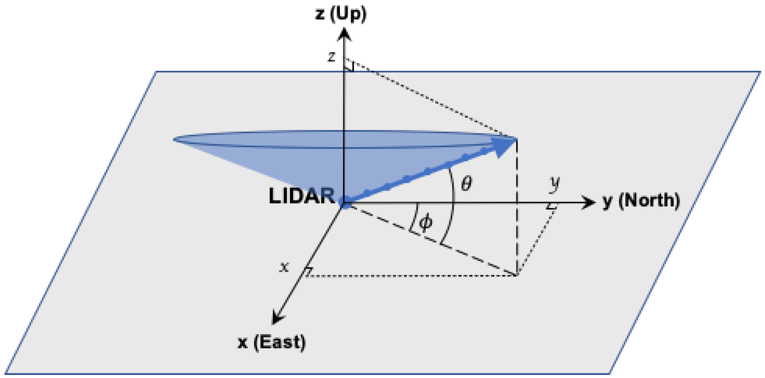
2.1. Doppler LiDAR Working Principle
2.2. Wind Field Remote Sensing for Wind Power Forecasting
3. Methodology
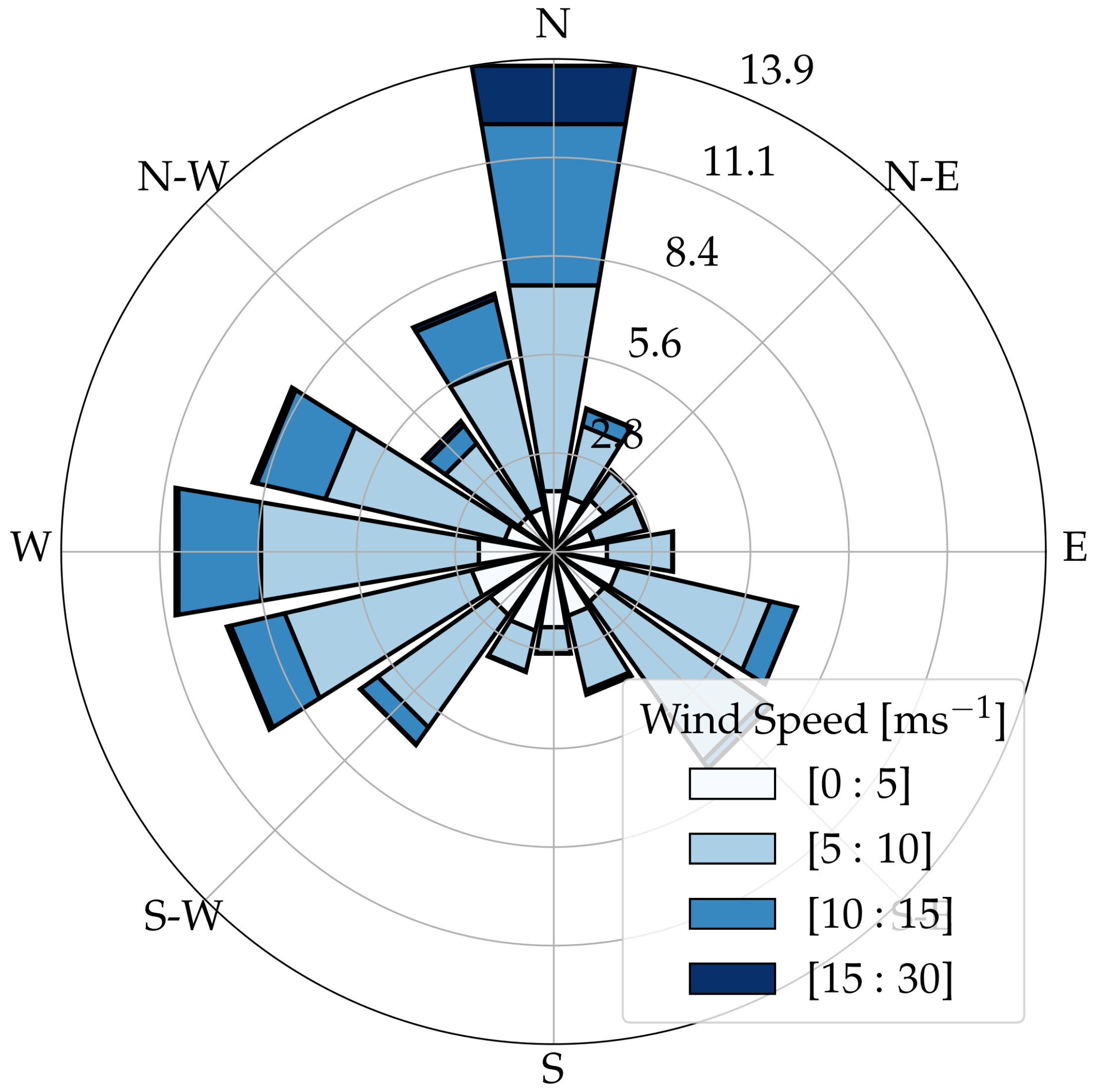
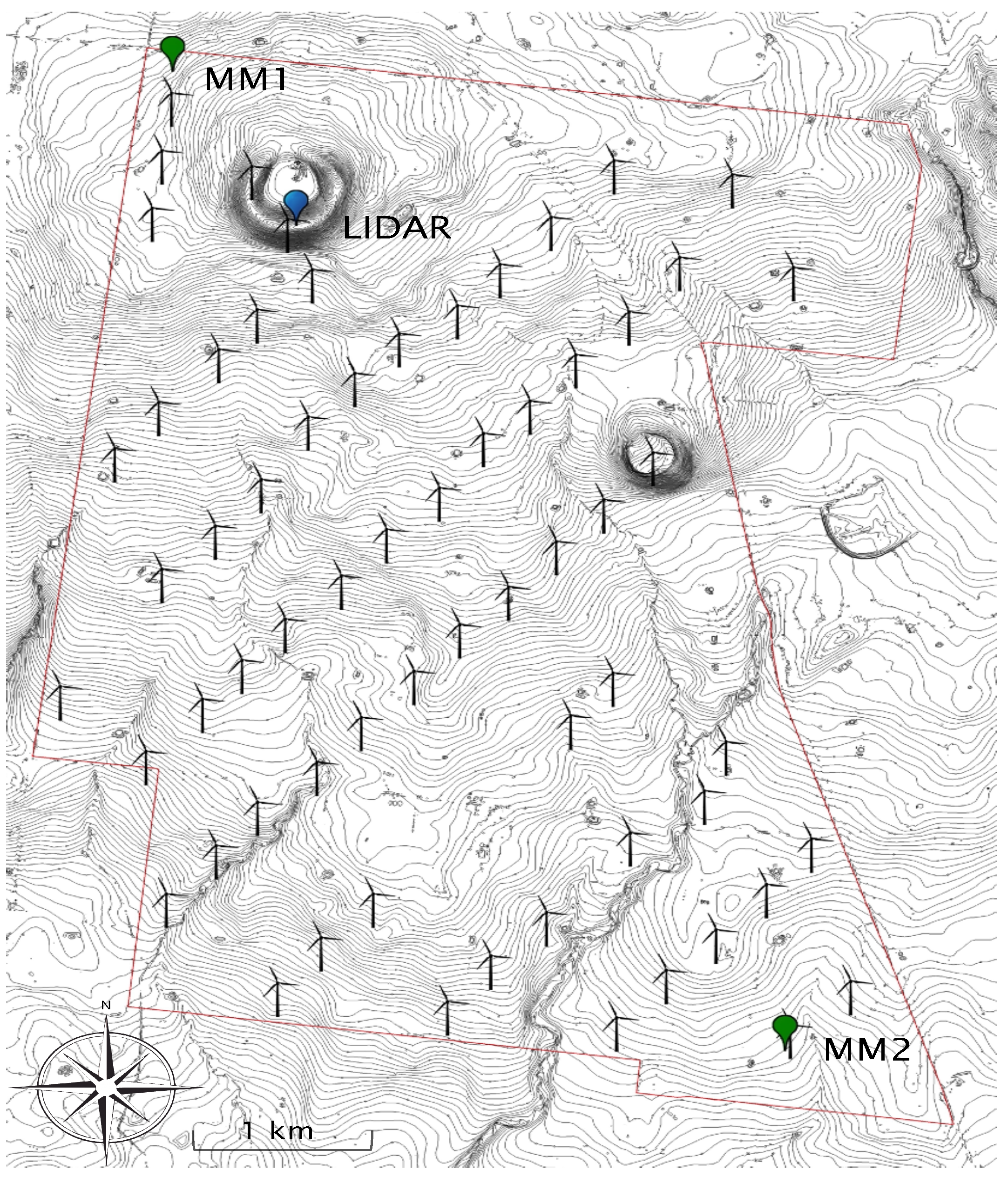
3.1. The Site and Data Collection
3.2. LiDAR Data Preprocessing
3.2.1. Filtering
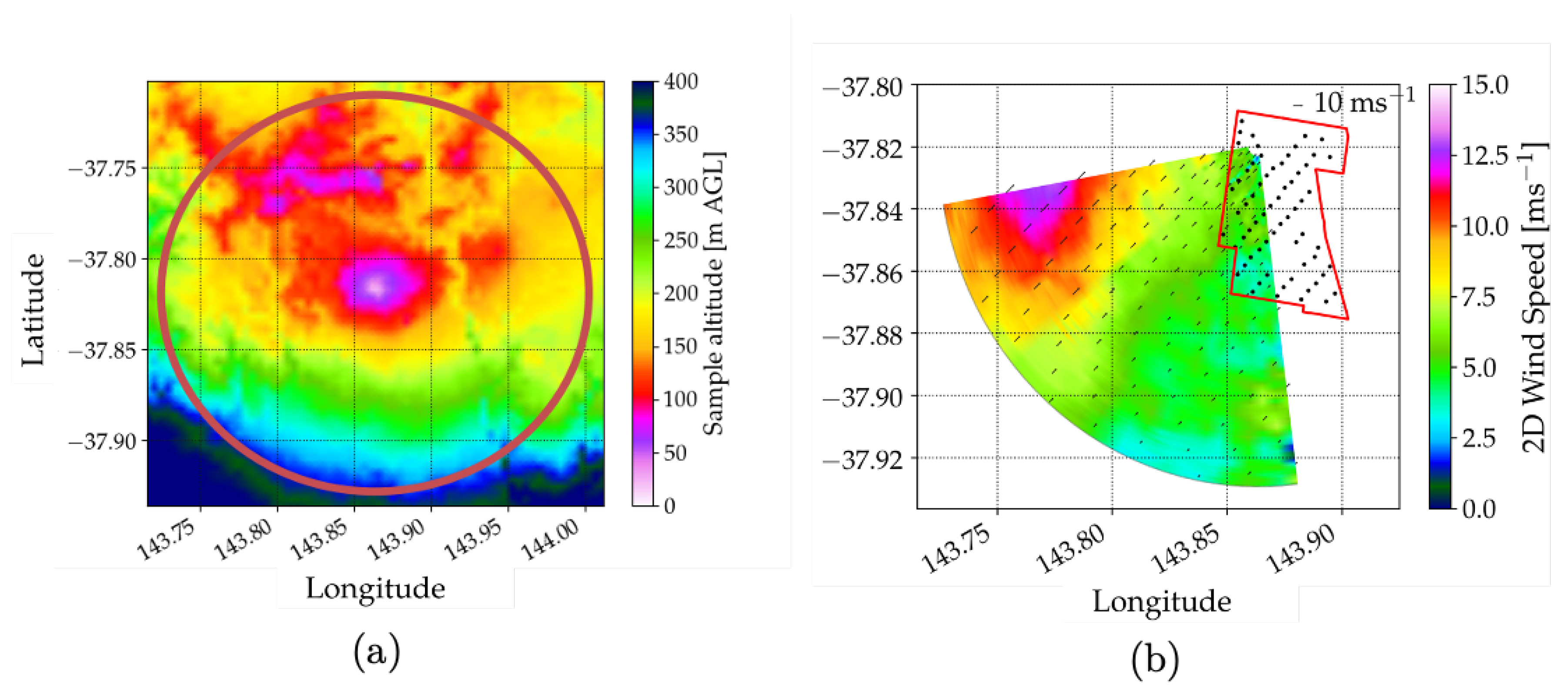
3.2.2. Wind Field Reconstruction
3.3. Forecast Algorithms
3.3.1. Benchmarks: Persistence and ARIMA
3.3.2. Smart Persistence
3.3.3. Deep Convolutional Neural Network
3.4. Model Evaluation
4. Results and Discussion
5. Conclusions
Author Contributions
Funding
Institutional Review Board Statement
Informed Consent Statement
Data Availability Statement
Acknowledgments
Conflicts of Interest
References
- EIA. Annual Energy Outlook 2019 with Projections to 2050; Technical Report; U.S. Department of Energy: Washington, DC, USA, 2019. [Google Scholar]
- GWEC. Global Wind Report 2019, Annual Market Update; Technical Report, GWEC: Brussels, Belgium, 2020. [Google Scholar]
- Kariniotakis, G. Renewable Energy Forecasting: From Models to Applications; Woodhead Publishing: Cambridge, UK, 2017. [Google Scholar]
- Wu, Z.; Gao, W.; Gao, T.; Yan, W.; Zhang, H.; Yan, S.; Wang, X. State-of-the-Art Review on Frequency Response of Wind Power Plants in Power Systems. J. Mod. Power Syst. Clean Energy 2018, 6, 1–16. [Google Scholar] [CrossRef]
- Vincent, C.L.; Trombe, P.J. Forecasting Intrahourly Variability of Wind Generation. In Renewable Energy Forecasting; Kariniotakis, G., Ed.; Woodhead Publishing Series in Energy; Woodhead Publishing: Sawston, UK, 2017; pp. 219–233. [Google Scholar] [CrossRef]
- Naemi, M.; Brear, M.J. A Hierarchical, Physical and Data-Driven Approach to Wind Farm Modelling. Renew. Energy 2020, 162, 1195–1207. [Google Scholar] [CrossRef]
- Gallego, C.; Cuerva-Tejero, A.; Lopez-Garcia, O. A Review on the Recent History of Wind Power Ramp Forecasting. Renew. Sustain. Energy Rev. 2015, 52, 1148–1157. [Google Scholar] [CrossRef]
- Tayal, D. Achieving High Renewable Energy Penetration in Western Australia Using Data Digitisation and Machine Learning. Renew. Sustain. Energy Rev. 2017, 80, 1537–1543. [Google Scholar] [CrossRef]
- EPEXSPOT. Basics of the Power Market, Intra-Day Lead Times. 2020. Available online: https://www.epexspot.com/en/basicspowermarket (accessed on 13 May 2020).
- AEMC. Five Minute Settlement, Final Determination; Rule Determination ERC0201; Australian Energy Market Comission: Sydney, Australia, 2017. [Google Scholar]
- Tascikaraoglu, A.; Uzunoglu, M. A Review of Combined Approaches for Prediction of Short-Term Wind Speed and Power. Renew. Sustain. Energy Rev. 2014, 34, 243–254. [Google Scholar] [CrossRef]
- Wurth, I.; Valldecabres, L.; Simon, E.; Möhrlen, C.; Uzunoğlu, B.; Gilbert, C.; Giebel, G.; Schlipf, D.; Kaifel, A. Minute-Scale Forecasting of Wind Power—Results from the Collaborative Workshop of IEA Wind Task 32 and 36. Energies 2019, 12, 712. [Google Scholar] [CrossRef]
- Hirth, B.D.; Schroeder, J.L.; Irons, Z.; Walter, K. Dual-Doppler Measurements of a Wind Ramp Event at an Oklahoma Wind Plant. Wind Energy 2016, 19, 953–962. [Google Scholar] [CrossRef]
- Frehlich, R. Scanning Doppler LiDAR for Input into Short-Term Wind Power Forecasts. J. Atmos. Ocean. Technol. 2013, 30, 230–244. [Google Scholar] [CrossRef]
- Valldecabres, L.; Nygaard, N.; von Bremen, L.; Kühn, M. Very Short-Term Probabilistic Forecasting of Wind Power Based on Dual-Doppler Radar Measurements in the North Sea. In Journal of Physics: Conference Series; IOP Publishing: Bristol, UK, 2018; Volume 1037, p. 052010. [Google Scholar] [CrossRef]
- Hirth, B.D.; Schroeder, J.L.; Gunter, W.S.; Guynes, J.G. Coupling Doppler Radar-Derived Wind Maps with Operational Turbine Data to Document Wind Farm Complex Flows. Wind Energy 2015, 18, 529–540. [Google Scholar] [CrossRef]
- Magerman, B. Short-Term Wind Power Forecasts Using Doppler LiDAR. Ph.D. Thesis, Arizona State University, Tempe, AZ, USA, 2014. [Google Scholar]
- Carpenter, R.L.; Shaw, B.; Margulis, M.; Barr, K.; Yates, D. Short-Term Numerical Forecasts Using WindTracer LiDAR Data. In Proceedings of the Fourth Conference on Weather, Climate, and the New Energy Economy, Austin, TX, USA, 7–10 January 2013. [Google Scholar]
- Valldecabres, L.; Peña, A.; Courtney, M.; von Bremen, L.; Kühn, M. Very Short-Term Forecast of near-Coastal Flow Using Scanning LiDARs. Wind Energy Sci. 2018, 3, 313–327. [Google Scholar] [CrossRef]
- Simon, E.I. Minute-Scale Wind Forecasting Using LiDAR Inflow Measurements. Ph.D. Thesis, DTU Wind Energy, DTU University, Lyngby, Denmark, 2019. [Google Scholar]
- Simon, E.I.; Courtney, M. Minute-Scale Wind Vector Forecasting Using Scanning LiDAR Inputs to a Convolutional LSTM Neural Network (Draft in Preparation for Submission). Ph.D. Thesis, DTU University, Lyngby, Denmark, 2019. [Google Scholar]
- Wurth, I.; Ellinghaus, S.; Wigger, M.; Niemeier, M.J.; Clifton, A.; Cheng, P.W. Forecasting Wind Ramps: Can Long-Range LiDAR Increase Accuracy? J. Physics Conf. Ser. 2018, 1102, 012013. [Google Scholar] [CrossRef]
- Simon, E.; Courtney, M.; Vasiljevic, N. Minute-Scale Wind Speed Forecasting Using Scanning LiDAR Inflow Measurements. Wind. Energy Sci. Discuss. 2018, 1–30. [Google Scholar] [CrossRef]
- Potter, C.; Grimit, E.; Nijssen, B. Potential Benefits of a Dedicated Probabilistic Rapid Ramp Event Forecast Tool. In Proceedings of the 2009 IEEE/PES Power Systems Conference and Exposition, Seattle, WA, USA, 2009; Volume 10614365, pp. 1–5. [Google Scholar] [CrossRef]
- Trombe, P.J.; Pinson, P.; Madsen, H. A General Probabilistic Forecasting Framework for Offshore Wind Power Fluctuations. Energies 2012, 5, 621–657. [Google Scholar] [CrossRef]
- Valldecabres, L.; Gayle Nygaard, N.; Vera-Tudela, L.; Bremen, L.; Kühn, M. On the Use of Dual-Doppler Radar Measurements for Very Short-Term Wind Power Forecasts. Remote Sens. 2018, 10, 1701. [Google Scholar] [CrossRef]
- Valldecabres, L.; von Bremen, L.; Kühn, M. Minute-Scale Detection and Probabilistic Prediction of Offshore Wind Turbine Power Ramps Using Dual-Doppler Radar. Wind Energy 2020, 23, 2202–2224. [Google Scholar] [CrossRef]
- Theuer, F.; van Dooren, M.F.; von Bremen, L.; Kühn, M. Minute-Scale Power Forecast of Offshore Wind Turbines Using Long-Range Single-Doppler LiDAR Measurements. Wind Energy Sci. 2020, 5, 1449–1468. [Google Scholar] [CrossRef]
- Reuter, H.; Nelson, A.; Jarvis, A. An evaluation of void-filling interpolation methods for SRTM data. Int. J. Geogr. Inf. Sci. 2007, 21, 983–1008. [Google Scholar] [CrossRef]
- Pichault, M.; Vincent, C.; Skidmore, G.; Monty, J.; Holcombe, A.; Brear, M. Windcube 400S Dynamic Scanning Data Set. Figshare 2021. [Google Scholar] [CrossRef]
- Pearson, G.; Davies, F.; Collier, C. An Analysis of the Performance of the UFAM Pulsed Doppler LiDAR for Observing the Boundary Layer. J. Atmos. Ocean. Technol. 2009, 26, 240–250. [Google Scholar] [CrossRef]
- Kumer, V.M.; Reuder, J.; Furevik, B.R. A Comparison of LiDAR and Radiosonde Wind Measurements. Energy Procedia 2014, 53, 214–220. [Google Scholar] [CrossRef]
- Cheynet, E.; Jakobsen, J.B.; Snæbjörnsson, J.; Reuder, J.; Kumer, V.; Svardal, B. Assessing the Potential of a Commercial Pulsed LiDAR for Wind Characterisation at a Bridge Site. J. Wind Eng. Ind. Aerodyn. 2017, 161, 17–26. [Google Scholar] [CrossRef]
- Vasiljevic, N.; Palma, J.M.L.M.; Angelou, N.; Matos, J.C.; Menke, R.; Lea, G.; Mann, J.; Courtney, M.; Ribeiro, L.F.; Gomes, V.M.M.G.C. Perdigao 2015: Methodology for Atmospheric Multi-Doppler LiDAR Experiments. Atmos. Meas. Tech. Discuss. 2017, 10, 3463–3483. [Google Scholar] [CrossRef]
- Han, Y.; Liu, J.; Sun, D.; Han, F.; Zhou, A.; Zhao, R.; Xue, X.; Chen, T.; Zhen, F.; Lu, Y. Fine Gust Front Structure Observed by Coherent Doppler LiDAR at Lanzhou Airport (103°49′ E, 36°03′ N). Appl. Opt. 2020, 59, 2686. [Google Scholar] [CrossRef]
- Clifton, A.; Clive, P.; Gottschall, J.; Schlipf, D.; Simley, E.; Simmons, L.; Stein, D.; Trabucchi, D.; Vasiljevic, N.; Würth, I. IEA Wind Task 32: Wind LiDAR Identifying and Mitigating Barriers to the Adoption of Wind LiDAR. Remote Sens. 2018, 10, 406. [Google Scholar] [CrossRef]
- Pedregosa, F.; Varoquaux, G.; Gramfort, A.; Michel, V.; Thirion, B.; Grisel, O.; Blondel, M.; Prettenhofer, P.; Weiss, R.; Dubourg, V.; et al. Scikit-Learn: Machine Learning in Python. J. Od Mach. Learn. Res. 2011, 12, 2825–2830. [Google Scholar]
- Towers, P.; Jones, B.L. Real-Time Wind Field Reconstruction from LiDAR Measurements Using a Dynamic Wind Model and State Estimation. Wind Energy 2016, 19, 133–150. [Google Scholar] [CrossRef]
- Browning, K.A.; Wexler, R. The Determination of Kinematic Properties of a Wind Field Using Doppler Radar. J. Appl. Meteorol. 1968, 7, 105–113. [Google Scholar] [CrossRef]
- Lhermitte, R.M.; Atlas, D. Precipitation Motion by Pulse Doppler Radar. In Proceedings of the Ninth Weather Radar Conference, Kansas City, MO, USA, 23–26 October 1961; Meteor. Soc.: Boston, MA, USA, 1961; pp. 218–223. [Google Scholar]
- Cherukuru, N.W. Atmospheric Data Visualization in Mixed/Augmented Reality. Ph.D. Thesis, Arizona State University, Tempe, Arizona, 2017. [Google Scholar]
- Chang, W.Y. Short-Term Wind Power Forecasting Using the Enhanced Particle Swarm Optimization Based Hybrid Method. Energies 2013, 6, 4879–4896. [Google Scholar] [CrossRef]
- Box, G.E.P. Time Series Analysis; Forecasting and Control; Holden-Day: San Francisco, CA, USA, 1970. [Google Scholar]
- Hyndman, R.J.; Khandakar, Y. Automatic Time Series Forecasting: The Forecast Package for R. J. Stat. Softw. 2008, 27, 1–22. [Google Scholar] [CrossRef]
- Dickey, D.A.; Fuller, W.A. Distribution of the Estimators for Autoregressive Time Series With a Unit Root. J. Am. Stat. Assoc. 1979, 74, 427–431. [Google Scholar] [CrossRef]
- Akaike, H. A New Look at the Statistical Model Identification. IEEE Trans. Autom. Control 1974, 19, 716–723. [Google Scholar] [CrossRef]
- Smith, T.G. Pmdarima: ARIMA Estimators for Python. 2017. Available online: http://www.alkaline-ml.com/pmdarima (accessed on 1 December 2020).
- Notton, G.; Voyant, C. Forecasting of Intermittent Solar Energy Resource. In Advances in Renewable Energies and Power Technologies; Elsevier: Amsterdam, The Netherlands, 2018; pp. 77–114. [Google Scholar] [CrossRef]
- Kumler, A.; Xie, Y.; Zhang, Y. A New Approach for Short-Term Solar Radiation Forecasting Using the Estimation of Cloud Fraction and Cloud Albedo; Technical Report TP–5D00-72290, 1476449; NREL: Golden, CO, USA, 2018. [Google Scholar] [CrossRef]
- Tato, J.; Brito, M. Using Smart Persistence and Random Forests to Predict Photovoltaic Energy Production. Energies 2018, 12, 100. [Google Scholar] [CrossRef]
- Taylor, G.I. The Spectrum of Turbulence. Proc. R. Soc. Lond. Ser. A 1938, 164, 476–490. [Google Scholar] [CrossRef]
- Germann, U.; Zawadzki, I. Scale-Dependence of the Predictability of Precipitation from Continental Radar Images. Part I: Description of the Methodology. Mon. Weather Rev. 2002, 130, 2859–2873. [Google Scholar] [CrossRef]
- Zhou, K.; Cherukuru, N.; Sun, X.; Calhoun, R. Wind Gust Detection and Impact Prediction for Wind Turbines. Remote Sens. 2018, 10, 514. [Google Scholar] [CrossRef]
- Rumelhart, D.E.; Hinton, G.E.; Williams, R.J. Learning Representations by Back-Propagating Errors. Nature 1986, 323, 533–536. [Google Scholar] [CrossRef]
- Nair, V.; Hinton, G.E. Rectified Linear Units Improve Restricted Boltzmann Machines. In Proceedings of the 27th International Conference on International Conference on Machine Learning, ICML’10; Haifa, Israel, 21–24 June 2010, Omnipress: Madison, WI, USA, 2010; pp. 807–814. [Google Scholar]
- Li, Z.; Yang, W.; Peng, S.; Liu, F. A Survey of Convolutional Neural Networks: Analysis, Applications, and Prospects. arXiv 2020, arXiv:2004.02806. [Google Scholar]
- Goodfellow, I.; Bengio, Y.; Courville, A. Deep Learning; MIT Press: Cambridge, MA, USA, 2016. [Google Scholar]
- Simonyan, K.; Zisserman, A. Very Deep Convolutional Networks for Large-Scale Image Recognition. arXiv 2015, arXiv:1409.1556. [Google Scholar]
- Chollet, F. Deep Learning with Python; Manning Publications Co.: Shelter Island, NY, USA, 2018. [Google Scholar]
- Abadi, M.; Agarwal, A.; Barham, P.; Brevdo, E.; Chen, Z.; Citro, C.; Corrado, G.S.; Davis, A.; Dean, J.; Devin, M.; et al. TensorFlow: Large-Scale Machine Learning on Heterogeneous Distributed Systems. arXiv 2015, arXiv:1603.04467. [Google Scholar]
- Meade, B.; Lafayette, L.; Sauter, G.; Tosello, D. Spartan HPC-Cloud Hybrid: Delivering Performance and Flexibility. Univ. Melb. 2017. [Google Scholar] [CrossRef]
- Dauphin, Y.N. RMSProp and Equilibrated Adaptive Learning Rates for Non-Convex Optimization. arXiv 2015, arXiv:1502.04390. [Google Scholar]
- Ruder, S. An Overview of Gradient Descent Optimization Algorithms. arXiv 2017, arXiv:1609.04747. [Google Scholar]
- Kingma, D.P.; Ba, J. Adam: A Method for Stochastic Optimization. arXiv 2017, arXiv:1412.6980. [Google Scholar]
- Dozat, T. Incorporating Nesterov Momentum into ADAM. In Proceedings of the ICLR 2016, San Juan, Puerto Rico, 2–4 May 2016; p. 4. [Google Scholar]
- Willmott, C.; Matsuura, K. Advantages of the Mean Absolute Error (MAE) over the Root Mean Square Error (RMSE) in Assessing Average Model Performance. Clim. Res. 2005, 30, 79–82. [Google Scholar] [CrossRef]
- Zoumakis, N.M.; Kelessis, A.G. The Dependence of the Bulk Richardson Number on Stability in the Surface Layer. Bound. Layer Meteorol. 1991, 57, 407–414. [Google Scholar] [CrossRef]
- Grachev, A.A.; Fairall, C.W. Dependence of the Monin–Obukhov Stability Parameter on the Bulk Richardson Number over the Ocean. J. Appl. Meteorol. 1997, 36, 406–414. [Google Scholar] [CrossRef]
- Holtslag, M.C.; Bierbooms, W.A.A.M.; van Bussel, G.J.W. Estimating Atmospheric Stability from Observations and Correcting Wind Shear Models Accordingly. J. Physics Conf. Ser. 2014, 555, 012052. [Google Scholar] [CrossRef]
- Pichault, M.; Vincent, C.; Skidmore, G.; Monty, J. Characterisation of Intra-Hourly Wind Power Ramps at the Wind Farm Scale and Associated Processes. Wind Energy Sci. 2021, 6, 131–147. [Google Scholar] [CrossRef]
- Powell, D.C.; Elderkin, C.E. An Investigation of the Application of Taylor’s Hypothesis to Atmospheric Boundary Layer Turbulence. J. Atmos. Sci. 1974, 31, 990–1002. [Google Scholar] [CrossRef]


| Parameter | WindCube 400S |
|---|---|
| Beam wavelength | 1.54 μm |
| Pulse repetition frequency | 10 kHz |
| Accumulation time | 1 s |
| Rotation speed | 3s |
| Velocity range | −30 to +30 ms |
| Elevation angle | 0.6 |
| Starting azimuth angle | variable |
| Final azimuth angle | variable |
| Display resolution | 75 m |
| Range gate length | 150 m |
| Number of gates | 159 |
| Maximum range | 12,250 m |
| Wind field sampling period | 33 s |
| Dynamic scanning adjustment period | 11 |
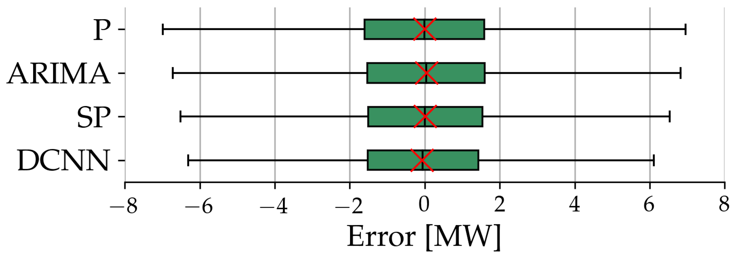
| Metric | P | ARIMA | SP | DCNN | |
|---|---|---|---|---|---|
| Err (MW) | 2.87 | 2.79 | 2.71 | 2.59 | |
| MAE | %DO | - | 84.93 | 79.45 | 87.67 |
| %DO | 15.07 | - | 67.12 | 71.23 | |
| Err (MW) | 4.75 | 4.60 | 4.48 | 4.26 | |
| RMSE | %DO | - | 80.82 | 80.82 | 90.41 |
| %DO | 19.18 | - | 65.75 | 75.34 |
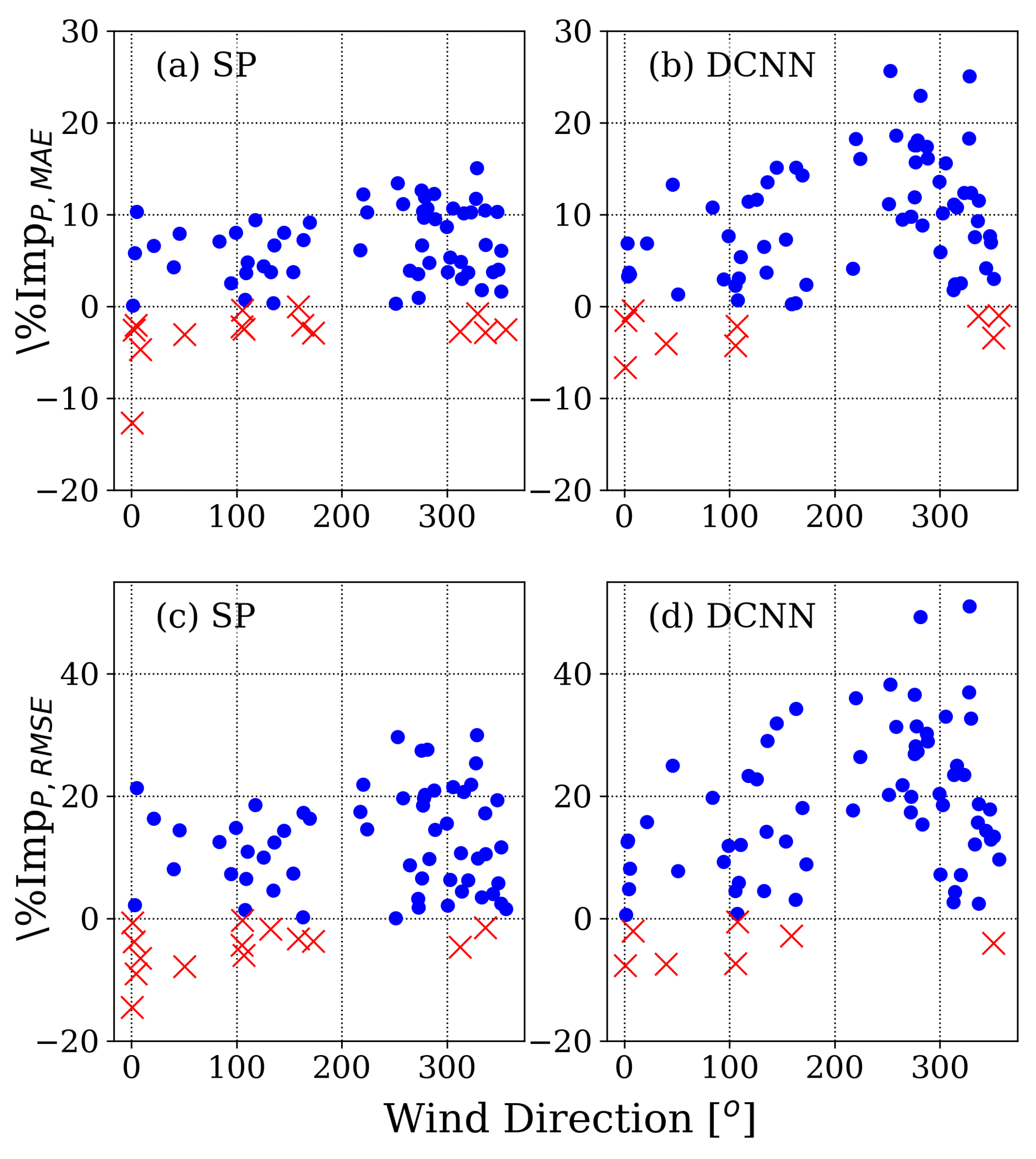
| %Imp | %Imp | %Imp | %Imp | ||||||
|---|---|---|---|---|---|---|---|---|---|
| SP | DCNN | SP | DCNN | SP | DCNN | SP | DCNN | ||
| Period | All | 5.74 | 9.74 | 5.82 | 10.37 | 3.12 | 7.22 | 2.61 | 7.31 |
| Ramp | 12.02 | 18.59 | 9.21 | 14.07 | 4.00 | 11.17 | 2.57 | 7.79 | |
| No-ramp | 4.93 | 8.58 | 4.62 | 9.06 | 3.01 | 6.74 | 2.62 | 7.16 | |
| Wind Sector | North | 3.36 | 4.92 | 3.87 | 5.73 | 2.00 | 3.58 | 1.41 | 3.31 |
| East | 5.28 | 4.92 | 5.88 | 6.09 | 2.09 | 1.72 | 3.08 | 3.30 | |
| South | 5.40 | 11.30 | 6.33 | 13.50 | 1.80 | 7.93 | 2.04 | 9.54 | |
| West | 7.89 | 14.73 | 6.96 | 13.55 | 4.69 | 11.77 | 3.42 | 10.26 | |
| Stability Condition | Stable | 5.36 | 8.03 | 4.63 | 7.57 | 2.33 | 5.09 | 1.27 | 4.32 |
| Unstable | 5.46 | 10.68 | 5.19 | 11.44 | 1.72 | 7.15 | 1.24 | 7.75 | |
| Neutral | 7.10 | 13.04 | 9.14 | 15.83 | 6.74 | 12.71 | 6.89 | 13.74 | |
| MAE | RMSE | FA | RC | CSI | ||||
|---|---|---|---|---|---|---|---|---|
| (MW) | (MW) | (%) | (%) | (%) | (MW) | (min) | (min) | |
| P | 9.91 | 13.41 | 97.73 | 100 | 97.73 | 0.18 | 5.05 | 0.16 |
| ARIMA | 9.08 | 12.50 | 95.56 | 100 | 95.56 | 2.73 | 4.82 | 1.96 |
| SP | 8.72 | 12.18 | 89.66 | 90.70 | 82.11 | 3.30 | 5.47 | 3.52 |
| CNN | 8.06 | 11.53 | 86.05 | 86.05 | 75.51 | 4.89 | 5.73 | 4.23 |
Publisher’s Note: MDPI stays neutral with regard to jurisdictional claims in published maps and institutional affiliations. |
© 2021 by the authors. Licensee MDPI, Basel, Switzerland. This article is an open access article distributed under the terms and conditions of the Creative Commons Attribution (CC BY) license (https://creativecommons.org/licenses/by/4.0/).
Share and Cite
Pichault, M.; Vincent, C.; Skidmore, G.; Monty, J. Short-Term Wind Power Forecasting at the Wind Farm Scale Using Long-Range Doppler LiDAR. Energies 2021, 14, 2663. https://doi.org/10.3390/en14092663
Pichault M, Vincent C, Skidmore G, Monty J. Short-Term Wind Power Forecasting at the Wind Farm Scale Using Long-Range Doppler LiDAR. Energies. 2021; 14(9):2663. https://doi.org/10.3390/en14092663
Chicago/Turabian StylePichault, Mathieu, Claire Vincent, Grant Skidmore, and Jason Monty. 2021. "Short-Term Wind Power Forecasting at the Wind Farm Scale Using Long-Range Doppler LiDAR" Energies 14, no. 9: 2663. https://doi.org/10.3390/en14092663
APA StylePichault, M., Vincent, C., Skidmore, G., & Monty, J. (2021). Short-Term Wind Power Forecasting at the Wind Farm Scale Using Long-Range Doppler LiDAR. Energies, 14(9), 2663. https://doi.org/10.3390/en14092663