Minimizing Stochastic Complexity with Ridge Regression

Abstract

We derive a penalty strength criterion for ridge regression using stochastic complexity, which is a refined variant of the minimum description length principle. Since stochastic complexity does not typically account for the effect of regularization on complexity, despite its ability to simplify models, we are required to make a slight modification to the underlying coding scheme. Our scheme makes use of a weighted ensemble of regularized model fits rather than a mixture of maximum likelihood estimates. Under this modification, regularization is interpreted as reducing model complexity by constraining flexibility. In the case of ridge regression, the complexity penalty term that we derive can be expressed analytically as the log determinant of the residual operator. We demonstrate the effect of this complexity penalty by fitting a linear readout to a reservoir computer, and by performing benchmark testing on publicly available datasets.

1. Introduction

We approach the problem of selecting a regularization strength for ridge regression with the intent of producing the simplest generalized linear model (GLM). This complexity-based approach is particularly relevant since the popularity of GLMs stems, in part, from their simplicity as a model class [1,2,3,4,5]. They are often used to identify and characterize relationships from data in fields like medicine [6,7], dietary science [8], economics [9,10], and sociology [11,12]. Such applications lie in accordance with Occam’s razor principle, which tells us to seek simple explanations, or in this case, simple model classes.

In these endeavours, it is common to use some form of regularization in the fitting process, like an L2 ridge penalty. In the case of ridge regularization, the penalty term stabilizes the matrix inverse under multicollinearity of input variables [3,13,14] and improves generalization to new data by reducing model variance at the expense of increased model bias [15,16,17]. The application of regularization also further reduces the complexity of linear models. This makes it possible to choose the regularization strength that minimizes model complexity.

In this paper, we measure complexity in terms of stochastic complexity [18], which is a refined variant of the minimum description length principle [19] (MDL). The stochastic complexity of a model is directly related to its flexibility. When used for model selection, it suggests that we should hesitate to choose a model class that fits our dataset well if it also provides good fits to unrelated datasets using the same predictors. While regularization constrains flexibility and produces simpler models, this is not directly accounted for by stochastic complexity. As such, the purpose of this paper, as well as deriving a ridge strength criterion, is to demonstrate a method for determining the effect of regularization on the stochastic complexity of a model. Our method makes use of a novel interpretation of stochastic complexity’s underlying coding scheme in order to directly account for the constraint imposed by regularization on model flexibility.

Our work is organized as follows. In Section 2, we provide an overview of stochastic complexity, including an explanation of the typical underlying coding scheme. In Section 3, we discuss our method for modifying this scheme to account for regularization. In Section 4, we derive an analytical form for the stochastic complexity of a linear model fitted by ridge regression using our modified scheme. We also present our ridge penalty selection criterion. In Section 5, we compare our criterion with several other information-theoretic criteria. In particular, we note that our work is closely related to that of Dwivedi et al. [20], who recently used luckiness normalized maximum likelihood [21] (LNML) for ridge strength selection. Their approach produces a different selection criterion, which stems from a different interpretation of regularization’s effect on complexity. In Section 6, we discuss the effect of our modification on stochastic complexity’s underlying probability distribution. We then visualize this effect using a two-dimensional toy example. In Section 7, we use our criteria to train linear readouts with the example of reservoir computing. We also perform benchmark testing in Section 8 using more than one hundred publicly available datasets from the Penn Machine Learning Benchmark (PMLB) repository [22]. In Section 9, we conclude with a discussion and summary.

2. Background into Stochastic Complexity and the Minimum Description Length Principle

The premise behind MDL is that models compress information. This is done by making use of a parametric model class to derive a coding scheme for possible data sets. The shorter the encoding of the dataset we wish to model under the scheme we derive, the better the compression achieved by the model. For example, in classical two-part MDL, the scheme is to first encode our model parameters and then to encode the errors that the model makes using these parameters. The best models, according to two-part MDL, minimize the combined lengths of their error and parameter codes.

The coding scheme assumed by stochastic complexity is more abstract. No one set of model parameters is used. Instead, a probability $P_0^{\ast }(Y;\mathcal{M},X)$ is assigned to each potential dataset Y from the set of possibilities $Y\in \mathcal{Y}$ using a weighted ensemble of parameterizations from the same model class $\mathcal{M}:(X,\theta )\to Y$. If we denote the weighting associated with each parameterization $\theta$ in the ensemble as $\pi \left(\theta \right)$, then the probability assigned by the resulting ensemble would be equivalent to the marginal probability under $\pi$ as a prior

$$P_0^{\ast }(Y;\mathcal{M},X)=\sum _{\theta }P\left(Y\right|\theta ;\mathcal{M},X)\pi \left(\theta \right).$$

Importantly, the ensemble weightings are chosen deterministically based on the model class. This is what enables the resulting code to be deciphered and makes stochastic complexity a valid description length. Under the stochastic complexity scheme, ensemble weights $\pi \left(\theta \right)$ are chosen before the dataset Y is known in the way that minimizes regret for the worst possible scenario of Y. This regret $R_0(Y,P_0^{\ast })$ is the difference between the length of code assigned to Y by the weighted ensemble (which we denote by $L_{\mathrm{sc}}\left(Y\right)$) and the shortest length that could be used to encode Y with any other ensemble. Under the lower bound for efficiency given by Shannon’s source coding theorem, these code lengths are negative log probabilities $L_{\mathrm{sc}}(Y;\mathcal{M},X)=-\log \left(P_0^{\ast }\left(Y\right)\right)$. Since the best ensemble for encoding any particular dataset Y is just its maximum likelihood estimate ${\theta }_Y^{\ast }$, the worst-case regret which we seek to minimize by choice of weightings is the following

$$\begin{array}{cc}\hfill R_0^{\max }(Y,P_0^{\ast })& :=\underset{Y\in \mathcal{Y}}{\max }\left(R_0(Y,P_0^{\ast })\right),\hfill \end{array}$$

(1)

$$\begin{array}{cc}\hfill \mathrm{where}{R}_0(Y,P_0^{\ast })& :=-\log \left(P_0^{\ast }(Y;\mathcal{M},X)\right)+\log \left(P\left(Y\right|{\theta }_Y^{\ast };\mathcal{M},X)\right).\hfill \end{array}$$

(2)

The weightings that minimize this worst-case regret are those that induce proportionality to the maximum likelihood estimate ($P_0^{\ast }(Y;\mathcal{M},X)={\displaystyle \frac{1}{{\mathrm{C}}_0}}P\left(Y\right|{\theta }_Y^{\ast };\mathcal{M},X)$). This means that we can work directly with $P_0^{\ast }$ without ever actually determining the optimal weightings. Under proportionality, regret is constant across all datasets $R_0(Y_1,P_0^{\ast })=\log \left({\mathrm{C}}_0\right)\forall Y\in \mathcal{Y}$. The constant of proportionality ${\mathrm{C}}_0$ must be the sum of all maximum likelihoods in order for it to induce a properly normalized distribution that integrates to one. For this reason, $P_0^{\ast }$ is often called the normalized maximum likelihood (NML) distribution. The probability of Y under $P_0^{\ast }$ is given as follows

$$P_0^{\ast }(Y;\mathcal{M},X)={\displaystyle \frac{P\left(Y\right|{\theta }_Y^{\ast };\mathcal{M},X)}{{\sum }_{Y^{\prime }\in \mathcal{Y}}P\left(Y^{\prime }\right|{\theta }_{Y^{\prime }}^{\ast };\mathcal{M},X)}}.$$

(3)

When we work with continuous data, and therefore an infinite set of possible datasets $\mathcal{Y}$, the ensemble weights $\pi \left(\theta \right)$ become difficult to determine. They have been shown [4,23], to approach the Jeffreys prior [24] for large datasets under certain conditions [25]. However, we are not required to determine the ensemble weights since proportionality still holds, and we can again work directly with $P_0^{\ast }$. In the case of continuous data, the stochastic complexity makes use of the integral version for $P_0^{\ast }$

$$L_{\mathrm{SC}}(Y;\mathcal{M},X)=-\log {\displaystyle \frac{P\left(Y\right|{\theta }_Y^{\ast };\mathcal{M},X)}{{\int }_{Y^{\prime }\in \mathcal{Y}}P\left(Y^{\prime }\right|{\theta }_{Y^{\prime }}^{\ast };\mathcal{M},X)d{Y}^{\prime }}}.$$

(4)

Notice that stochastic complexity can be broken into two terms, the first being the model’s negative log likelihood. The other term measures the complexity of the parametric model class $\mathcal{M}$

$$\mathrm{Penalty}=\log \left({\int }_{Y^{\prime }\in \mathcal{Y}}P\left(Y^{\prime }\right|{\theta }_{Y^{\prime }}^{\ast };\mathcal{M},X)d{Y}^{\prime }\right),$$

and functions as the penalty term in model selection. This penalty directly measures flexibility and it lends stochastic complexity an important intuition beyond its meaning as a code length. It tells us not to trust models that fit the data well if they can also provide good fits to unrelated data using the same predictors.

3. The Effect of Regularization on Complexity

The role of model regularization on stochastic complexity can potentially be interpreted in different ways. Our interpretation is to directly consider the effect of regularization on the flexibility of the model class. This follows on from the intuitive meaning of stochastic complexity described in the previous section: that we should have more confidence in our regularized model if the regularization applied prevents the model from easily fitting unrelated datasets using the same predictors.

Rather than building a weighted ensemble of maximum likelihood estimates, we build a weighted ensemble of regularized fits. The weightings of this ensemble will depend on the regularization strength $\alpha$. We select the weightings such that the probability assigned by the ensemble $P_{\alpha }^{\ast }(Y;\mathcal{M},X)$ minimizes a modified form of regret in the worst case scenario. This modified regret, which we now denote by $R_{\alpha }(Y,P_{\alpha }^{\ast })$, because of its dependence on the regularization strength $\alpha$, is still the length of code that could have been saved had the parameter fit for the dataset been known ahead of time. The only difference is that this parameter fit is now the set of regularized parameters and not the maximum likelihood estimate

$$R_{\alpha }^{\max }(Y,P_{\alpha }^{\ast }):=\underset{Y\in \mathcal{Y}}{\max }\{-\log \left(P_{\alpha }^{\ast }(Y;\mathcal{M},X)\right)+\log \left(P\left(Y\right|{\theta }_{Y,\alpha }^{\ast };\mathcal{M},X)\right)\}.$$

Assuming that the encoder and decoder agree on the regularization strength ahead of time, they can calculate the ensemble probability $P_{\alpha }^{\ast }$ that minimizes this modified regret in the worst case choice of the data set $Y\in \mathcal{Y}$. We demonstrate in Appendix A that the solution is to choose $P_{\alpha }^{\ast }$ proportional to the likelihood at the regularized parameter fit $P_{\alpha }^{\ast }\left(Y\right)\propto P\left(Y\right|{\theta }_{Y,\alpha }^{\ast })$. The constant of proportionality is the normalization factor required to produce a distribution that integrates to unity. In the continuous case, the resulting NML distribution is defined as follows

$$P_{\alpha }^{\ast }(Y;\mathcal{M},X)={\displaystyle \frac{P\left(Y\right|{\theta }_{Y,\alpha }^{\ast };\mathcal{M},X)}{{\int }_{Y^{\prime }\in \mathcal{Y}}P\left(Y^{\prime }\right|{\theta }_{Y^{\prime },\alpha }^{\ast };\mathcal{M},X)d{Y}^{\prime }}},$$

(5)

while in the discrete case, the integral is replaced with a sum. Because the normalization factor ensures that $P_{\alpha }^{\ast }$ is a valid probability mass, it follows from Kraft’s inequality that a uniquely decodable scheme exists to describe the elements of $\mathcal{Y}$ with code word lengths between $-\log \left(P_{\alpha }^{\ast }\left(Y\right)\right)$ and $-\log \left(P_{\alpha }^{\ast }\left(Y\right)\right)+1$ nats (Ignoring fixed precision costs for continuous datasets). The scheme that achieves these code lengths is well defined for most model classes and types of regularization, which we discuss in Appendix B. The code lengths it assigns to datasets are given by the following

$$L_{\mathrm{SC}}(Y;\mathcal{M},X,\alpha )=-\log {\displaystyle \frac{P\left(Y\right|{\theta }_{Y,\alpha }^{\ast };\mathcal{M},X)}{{\int }_{Y^{\prime }\in \mathcal{Y}}P\left(Y^{\prime }\right|{\theta }_{Y^{\prime },\alpha }^{\ast };\mathcal{M},X)d{Y}^{\prime }}}.$$

(6)

One benefit of the model selection criterion that comes from this coding scheme ($L_{\mathrm{SC}}(Y;\mathcal{M},X,\alpha )$) is its generalizability. The criterion derived in Equation (6) is not specific to any particular model class or type of regularization. Another benefit is the fairness of the comparison it draws between regularization techniques. One technique can be compared with another based purely on how much each restricts the flexibility of the model class. The caveat, which is not unique to our approach, is that to derive an analytical value for stochastic complexity, we still need an analytical form for the model likelihood when regularization is applied.

4. Deriving a Ridge Penalty to Minimize Stochastic Complexity

In the case of regression with a known state matrix X, the parametric model class $\mathcal{M}$ is the multivariate normal distribution $\mathcal{N}(X\theta ,{ϵ}^2\mathbb{I})$. This is the model class for which the regression solution $\theta ={\theta }_Y^{\ast }$ provides the maximum likelihood estimate. From a Bayesian perspective, the ridge penalty comes from maximizing the posterior with the added assumption of a normal prior over the parameters. However, it is not strictly necessary to assume a prior over the parameters in order to calculate stochastic complexity. We only need to know the probability of each dataset $Y\in \mathcal{Y}$ given the regularized parameter fit ${\theta }_{Y,\alpha }^{\ast }$. According to our model class, that probability is the following

$$P\left(Y\right|{\theta }_{Y,\alpha }^{\ast };\mathcal{M},X)={\left(2\pi ϵ\right)}^{-n/2}\exp \left(-{\displaystyle \frac{\left|\right|Y-X{\theta }_{Y,\alpha }^{\ast }{\left|\right|}^2}{2{ϵ}^2}}\right).$$

Fortunately, an analytical form for this probability exists. First, we can express the ridge regression solution ${\theta }_{Y,\alpha }^{\ast }$ in terms of the penalty $\alpha$, the state matrix X and the dataset Y. It is given by ${\theta }_{Y,\alpha }^{\ast }={(X^{T}X+\alpha \mathbb{I})}^{-1}{X}^{T}Y$. This means that an analytical form for the mean square error (MSE), which we denote by ${\sigma }_{Y,\alpha }^2$, also exists

$$\begin{array}{cc}\hfill {\sigma }_{Y,\alpha }^2={\displaystyle \frac{1}{n}}{Y}^T{Q}_{\alpha }Y,\mathrm{where}{Q}_{\alpha }& ={(M_{\alpha }-\mathbb{I})}^T(M_{\alpha }-\mathbb{I})\hfill \\ \hfill \mathrm{and}{M}_{\alpha }& =X{(X^{T}X+\alpha \mathbb{I})}^{-1}{X}^T.\hfill \end{array}$$

In the expression above, n refers to the length of Y. We can use the matrix form for mean square error to rewrite the NML probability $P_{\alpha }^{\ast }\left(Y\right)$ in Equation (5) for the context of ridge regression

$$P_{\alpha }^{\ast }(Y;\mathcal{M})={\displaystyle \frac{{\left(2\pi ϵ\right)}^{-n/2}\exp (-\frac{Y^T{Q}_{\alpha }Y}{2{ϵ}^2})}{{\int }_{Y^{\prime }\in \mathcal{Y}}{\left(2\pi ϵ\right)}^{-n/2}\exp (-\frac{Y^{\prime }T{Q}_{\alpha }{Y}^{\prime }}{2{ϵ}^2})d{Y}^{\prime }}}.$$

(7)

The stochastic complexity then comes from taking the logarithm of this probability. The component corresponding to the complexity penalty is found by evaluating the integral in the denominator. For continuous datasets and linear models, it makes sense to take the space of possible datasets to be all real valued vectors of length n and set $\mathcal{Y}$ to ${\mathbb{R}}^n$

$$\log {\int }_{{\mathbb{R}}^n}{\left(2\pi {ϵ}^2\right)}^{-n/2}\exp (-{\displaystyle \frac{Y^T{Q}_{\alpha }Y}{2{ϵ}^2}})dY.$$

This integral then simplifies to the log determinant of $Q_{\alpha }^{-1/2}$

$$-{\displaystyle \frac{1}{2}}\log \left(\det \left(Q_{\alpha }\right)\right),$$

which can also be expressed in terms of the eigenvalues of the design matrix $X^{T}X$, denoted here by ${\lambda }_i$

$$-{\displaystyle \frac{1}{2}}\log \left(\det \left(Q_{\alpha }\right)\right)={\displaystyle \sum _{i=1}^m}\log (1+{\displaystyle \frac{{\lambda }_i}{\alpha }}).$$

This penalty describes how well we can fit various possible datasets using regression with a ridge constant of $\alpha$ and a gram matrix $X^{T}X$ that has the given spectrum $\{{\lambda }_1,{\lambda }_2,\dots {\lambda }_m\}$. Lastly, we need the other component of the stochastic complexity, which is the negative log of the numerator in Equation (7), and also the log likelihood of Y under its own parameter fit $-\log P\left(Y\right|{\theta }_{Y,\alpha }^{\ast };\mathcal{M},X)$. Together, the stochastic complexity becomes the following function of the ridge penalty:

$$L_{\mathrm{SC}}(Y;\mathcal{M},X,\alpha )={\displaystyle \frac{n}{2{ϵ}^2}}{\sigma }_{Y,\alpha }^2+{\displaystyle \sum _{i=1}^m}\log \left(1+{\displaystyle \frac{{\lambda }_i}{\alpha }}\right)+\mathrm{const}.$$

(8)

The constant term, which we ignore because it is irrelevant for our purpose, is $n\log \left(\sqrt{2\pi ϵ}\right)$.

The entries of the $m\times m$ gram matrix $X^{T}X$ scale proportionally to n, as do its eigenvalues ${\lambda }_i$. This means that in the asymptotic limit $n\to \infty$, the complexity penalty in Equation (8) can be written as follows

$${\displaystyle \sum _{i=1}^m}\log \left(1+{\displaystyle \frac{{\lambda }_i}{\alpha }}\right)\to {\displaystyle \sum _{i=1}^m}\log \left({\displaystyle \frac{{\lambda }_i}{\alpha }}\right)={\displaystyle \sum _{i=1}^m}\log \left({\lambda }_i\right)-m\log \left(\alpha \right),$$

Which is equivalent to the Bayesian information penalty

$${\displaystyle \sum _{i=1}^m}\log \left(1+{\displaystyle \frac{{\lambda }_i}{\alpha }}\right)\mathrm{scales}\mathrm{as}\mathcal{O}\left(1\right)+m\log \left(n\right).$$

This is a standard feature of MDL-derived selection criteria. We also demonstrate in Appendix C that the modified stochastic complexity in Equation (8) is universal in the expected sense [21]. This means that for any data-generating distribution from our parametric model class, the expected efficiency of our NML scheme is optimal in the asymptotic limit $n\to \infty$.

Calculating the stochastic complexity requires choosing a variance ${ϵ}^2$ for the multivariate Gaussian used in our coding scheme. This is also the case for various other ridge penalty criteria [26,27]. A typical method for doing so in the under-parameterized case ($m<<n$) is to estimate $ϵ$ in terms of the adjusted mean square error of the linear regression solution ${ϵ}^2=n{\sigma }_{Y,0}^2/(n-m)$. A more robust method, which is not limited to the under-parameterized case, is provided by Liu et al. [28]. They suggest approximating ${ϵ}^2$ by the following expression

$${ϵ}^2={\displaystyle \frac{Y^T(\mathbb{I}-M_{{\alpha }^{\prime }})Y}{n-\mathrm{Tr}\left(M_{{\alpha }^{\prime }}\right)}},$$

which makes use of the projection matrix $M_{{\alpha }^{\prime }}$. We denote the ridge strength used in this projection matrix by ${\alpha }^{\prime }$ to distinguish it from the strength $\alpha$ used in model training and the calculation of stochastic complexity.

Our formulation for optimizing the ridge penalty passes two sanity checks that we can construct from our understanding of ridge regression. Firstly, the optimal penalty scales correctly with the terms of the state matrix. If X is multiplied by a scalar $X\to c\ast X$, the optimal ridge penalty should scale proportionally to its square $\alpha \to c^2\alpha$, since this leaves the projection matrix $X{(X^{T}X+\alpha \mathbb{I})}^{-1}{X}^T$ unchanged. This is the case. The matrix $Q_{\alpha }$ is also invariant to the scaling $(X_{ij},\alpha )\to (c{X}_{ij},c^2\alpha )$, which means that the performance term ${\displaystyle \frac{n}{2ϵ}}{\sigma }_{Y,\alpha }^2={\displaystyle \frac{1}{2ϵ}}{Y}^T{Q}_{\alpha }Y$ and the complexity penalty $-{\displaystyle \frac{1}{2}}\log \left(\det \left(Q_{\alpha }\right)\right)$ are both unaffected. Secondly, since the penalty term is a measure of model flexibility, it should only depend on the unique, non-zero columns in X. This is also true. Duplicate columns, or columns of zeros, add eigenvalues of zero to the spectrum and these do not contribute to the penalty term.

5. Alternative Approaches

In Section 3, we accounted for regularization by devising a coding scheme from an ensemble of regularized parameter fits. An alternative approach is to build the ensemble from maximum posterior likelihood estimates after assuming a prior distribution over parameter space. This is similar to the way that luckiness normalized maximum likelihood (LNML) assumes a so-called ‘luckiness function’ $p_{\mathrm{luck}}\left(\theta \right)$ to derive a coding scheme which is optimized for the corresponding luckiness normalized probability density:

$$P_{\mathrm{LNML}}(Y;\mathcal{M},X):={\displaystyle \frac{{\max }_{\theta }\left[P\left(Y\right|\theta ;\mathcal{M},X)p_{\mathrm{luck}}\left(\theta \right)\right]}{{\int }_{Y^{\prime }\in \mathcal{Y}}{\max }_{\theta }\left[P\left(Y^{\prime }\right|\theta ;\mathcal{M},X)p_{\mathrm{luck}}\left(\theta \right)\right]d{Y}^{\prime }}}.$$

(9)

Dwivedi et al. [20] follow this approach and choose $p_{\mathrm{luck}}$ to be Gaussian

$$p_{\mathrm{luck}}\left(\theta \right)\propto \exp (-{\displaystyle \frac{\alpha }{2{ϵ}^2}}{\theta }^T\theta ).$$

This choice is meaningful because a Gaussian prior over the parameters produces a posterior likelihood which is maximal at the ridge regression solution. The numerator and denominator therefore both measure posterior likelihoods. Their resulting luckiness normalized likelihood can be expressed as follows

$$P_{\mathrm{Dwivedi}}(Y;\mathcal{M},X):={\displaystyle \frac{P\left(Y\right|{\theta }_{Y,\alpha }^{\ast };\mathcal{M},X)p_{\mathrm{luck}}\left({\theta }_{Y,\alpha }^{\ast }\right)}{{\int }_{Y^{\prime }\in \mathcal{Y}}P\left(Y^{\prime }\right|{\theta }_{Y^{\prime },\alpha }^{\ast };\mathcal{M},X)p_{\mathrm{luck}}\left({\theta }_{Y^{\prime },\alpha }^{\ast }\right)d{Y}^{\prime }}}.$$

(10)

The description length associated with this probability density, which we denote by $L_{\mathrm{Dwivedi}}$ and provide below, is similar to our own, but includes an additional log parameter likelihood term

$$L_{\mathrm{Dwivedi}}(Y;\mathcal{M},X,\alpha )={\displaystyle \frac{n}{2{ϵ}^2}}{\sigma }_{Y,\alpha }^2+{\displaystyle \frac{\alpha {\left({\theta }_{Y,\alpha }^{\ast }\right)}^T{\theta }_{Y,\alpha }^{\ast }}{2{ϵ}^2}}+{\displaystyle \frac{1}{2}}{\displaystyle \sum _{i=1}^m}\log (1+{\displaystyle \frac{{\lambda }_i}{\alpha }}).$$

The integral in the denominator also evaluates to half the value of the complexity penalty that we found from the denominator in Equation (7). This can be seen from the way that the prior and posterior probability factorize

$$\exp \left(-{\displaystyle \frac{1}{2ϵ}}{Y}^T{Q}_{\alpha }Y+\alpha {\left({\theta }_{Y,\alpha }^{\ast }\right)}^T{\theta }_{Y,\alpha }^{\ast }\right)=\exp \left(-{\displaystyle \frac{1}{2ϵ}}{Y}^T{Q}_{\alpha }^{1/2}Y\right).$$

The approach taken by Dwivedi et al. can be generalized to any regularization techniques that offer a Bayesian interpretation. The luckiness function would simply be replaced with whatever prior distribution is implicitly assumed over the parameters.

Another MDL-inspired approach taken by Silhavy et al. [29] makes use of a two-part coding scheme. They take the description length found for linear regression by Giurcaneanu et al. [30] and consider the additional cost of encoding the ridge parameter (or Lasso parameter). It should be noted that Giurcaneanu et al. found the description length for linear regression under a different framing of the model class. They encode the error variance ${\sigma }_{Y,\alpha =0}^2$ and then use the variance to encode the errors $Y\sim \mathcal{N}(X\theta ,{\sigma }_{Y,\alpha =0}^2\mathbb{I})$. As such, Silhavy et al.’s method for choosing an MDL ridge parameter is quite different than ours. They seek to minimize the following criterion

$$L_{\mathrm{Silhavy}}(Y;\mathcal{M},X,\alpha ):={\displaystyle \frac{n-k}{2}}\log \left({\sigma }_{Y,\alpha }^2\right)+{\displaystyle \frac{1}{2}}\log \left(\alpha \right)+{\displaystyle \frac{k}{2}}\log \left({\left({\theta }_{Y,\alpha }^{\ast }\right)}^T{X}^{T}X{\theta }_{Y,\alpha }^{\ast }\right)+\mathrm{const}.$$

(11)

It should also be noted that the major objective of Silhavy et al.’s work was to apply MDL to multi-criteria decision analysis. This means seeking a tradeoff between model complexity and a combination of various performance measures. In this paper, we only deal with a single objective, which is model log likelihood (effectively the mean square model error).

Other information criteria, like the Akaike [31] and Bayesian [32] Information Criteria (AIC and BIC, respectively), can also be used to choose a ridge strength if the number of model parameters is replaced with the number of effective degrees of freedom, which has dependence on $\alpha$ [33,34]. The commonly used measure of effective degrees of freedom is the trace of the projection matrix $M_{\alpha }=X{(X^{T}X+\alpha \mathbb{I})}^{-1}{X}^T$ [35,36]. This results in the modified AIC and BIC criteria provided below

$${\mathrm{AIC}}_{\mathrm{eff}}(Y;X,\alpha )={\displaystyle \frac{n}{{ϵ}^2}}{\sigma }_{Y,\alpha }^2+2{\displaystyle \sum _{i=1}^m}\left({\displaystyle \frac{{\lambda }_i}{{\lambda }_i+\alpha }}\right),\mathrm{and}$$

$${\mathrm{BIC}}_{\mathrm{eff}}(Y;X,\alpha )={\displaystyle \frac{n}{{ϵ}^2}}{\sigma }_{Y,\alpha }^2+\log \left(n\right){\displaystyle \sum _{i=1}^m}\left({\displaystyle \frac{{\lambda }_i}{{\lambda }_i+\alpha }}\right).$$

6. A Visualization of Probability Density on a Toy Problem

By modifying regret to account for regularization in Section 3, we alter the NML probability density $P_{\alpha }^{\ast }$ used to assign description lengths to datasets. This redistributes density towards the datasets whose likelihoods are reduced the least when switching from MLE parameters $P\left(Y\right|{\theta }_Y^{\ast })$ to regularized fits $P\left(Y\right|{\theta }_{Y,\alpha }^{\ast })$. 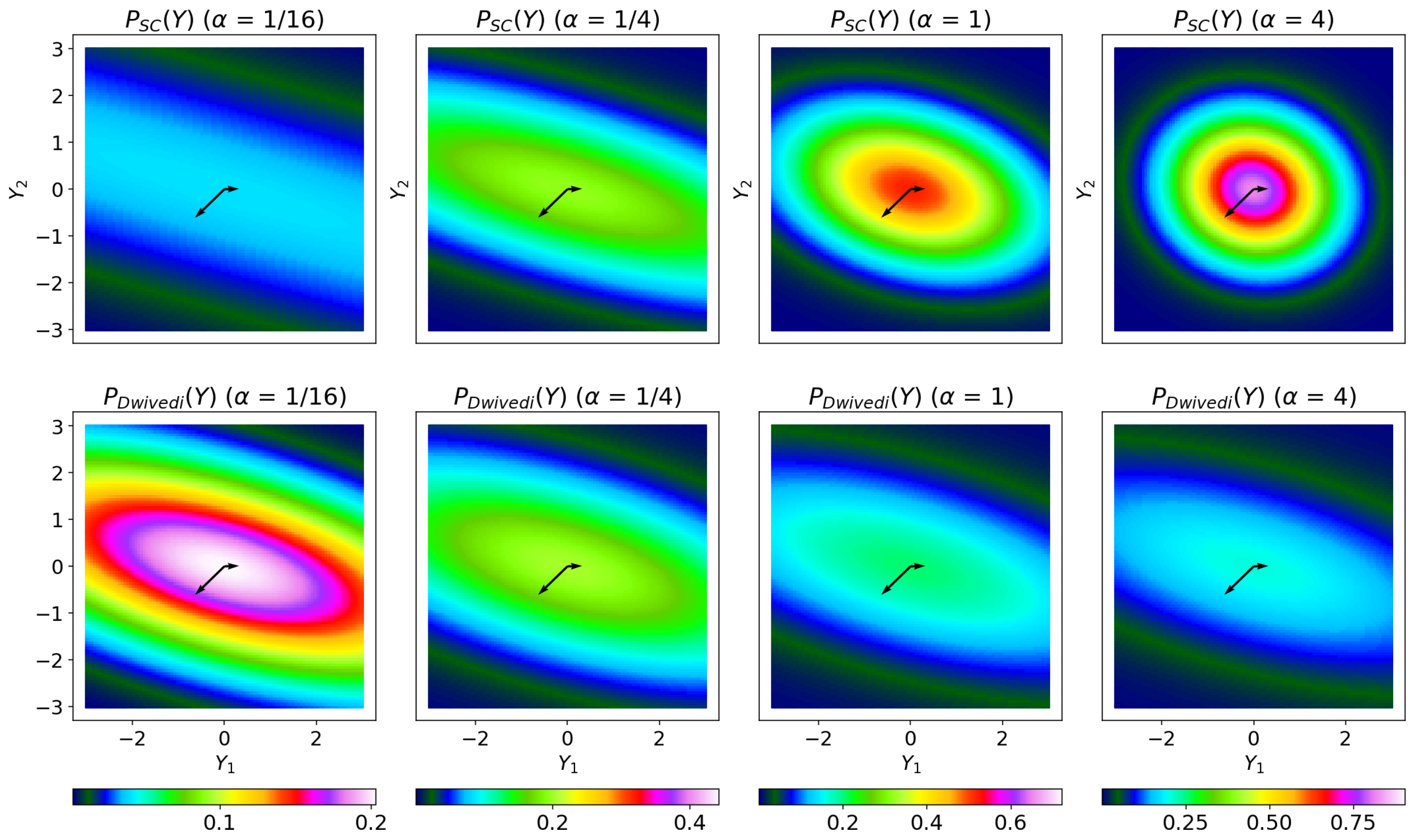In Figure 1, we visualize $P_{\alpha }^{\ast }$ on a toy example. We also visualize the LNML density used by Dwivedi et al. [20] for comparison. The example provided comes from fitting a linear model that maps the following $2\times 2$ input matrix

$$X=\left(\begin{array}{cc}-0.64& -0.61\\ 0.32& 0.01\end{array}\right),$$

to possible output datasets ($Y_1,Y_2$) in ${\mathbb{R}}^2$. The values in this example were generated by random sampling of the unit Gaussian and truncated to two decimal places.

When accounting for ridge regularization on linear models, $P_{\alpha }^{\ast }$ assigns equal probability density to the surfaces of the ellipsoids formed by the matrix $Q_{\alpha }$ (meaning the level sets of the quadratic form $Y^T{Q}_{\alpha }Y=\mathrm{Const}$). These are also surfaces of equal description length in dataset space. As the ridge penalty $\alpha$ is increased, these ellipsoids become smaller and more spherical. The density of $P_{\alpha }^{\ast }$ is increased close to the origin and decreased for datasets with large entries. However, more generally speaking, the geometry of $P_{\alpha }^{\ast }$ depends on the model class and the type of regularization performed.

7. Fitting a Reservoir Computer

As a proof of concept, we use our ridge penalty criterion to select a penalty strength for fitting reservoir computer readouts. Reservoir computers are high-dimensional dynamical systems that become conditionally stable when driven by an input signal. Their dynamic response is mapped to the future state of the input with a linear readout. This mapping is possible because the reservoir state-space becomes a time-delay embedding-space of the driving time series [37] according to the echo-state property [38,39], which reservoirs must satisfy. Reservoir readouts are often fitted with ridge regression [40,41,42] and their complexity is a subject of interest [5,43,44,45]. In particular, we use echo-state networks [38] (ESNs) as our reservoirs and perform time series prediction on Lorenz-96 [46]. Our exact method is detailed in Appendix D along with a description of echo-state networks.

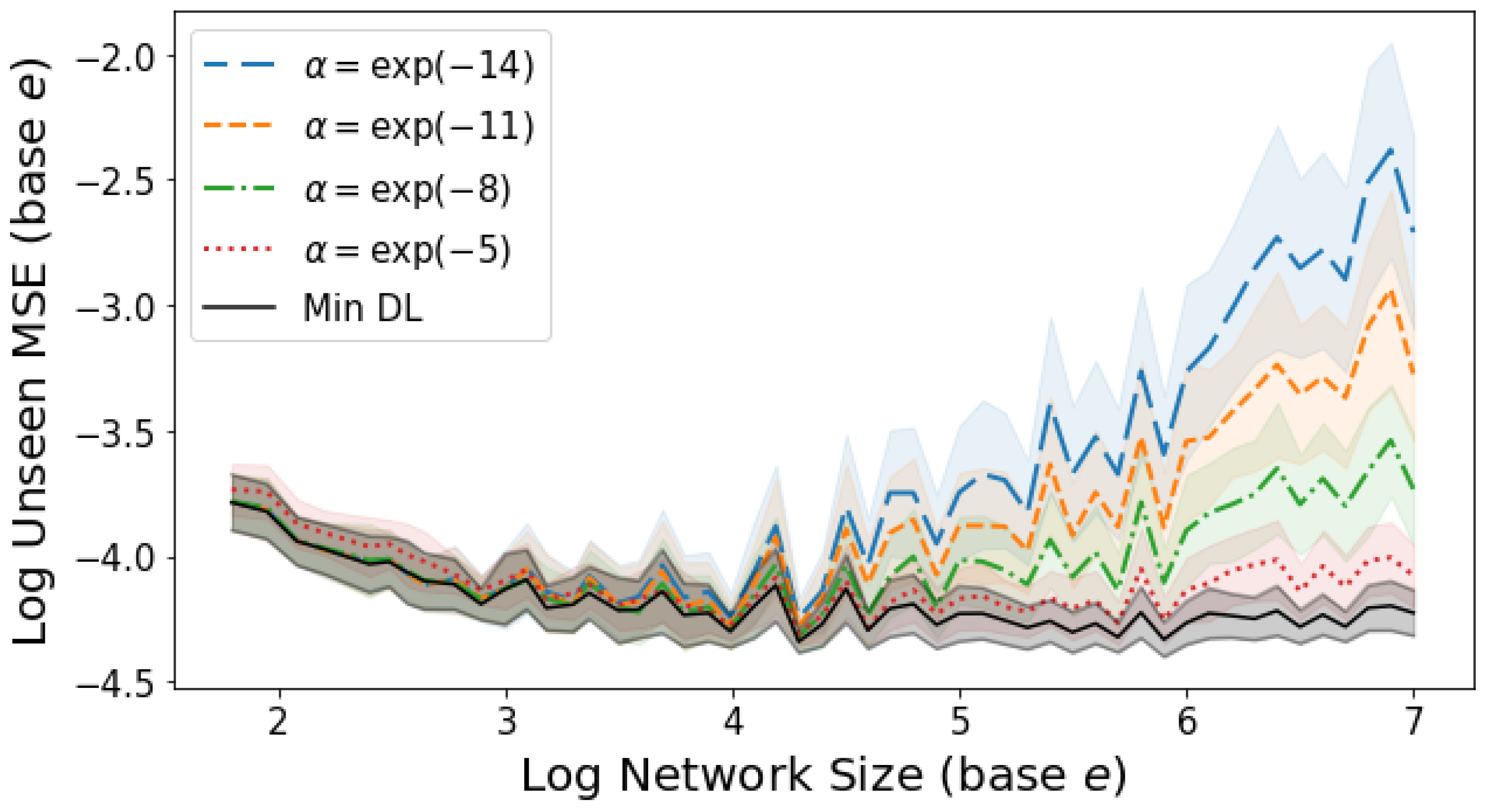
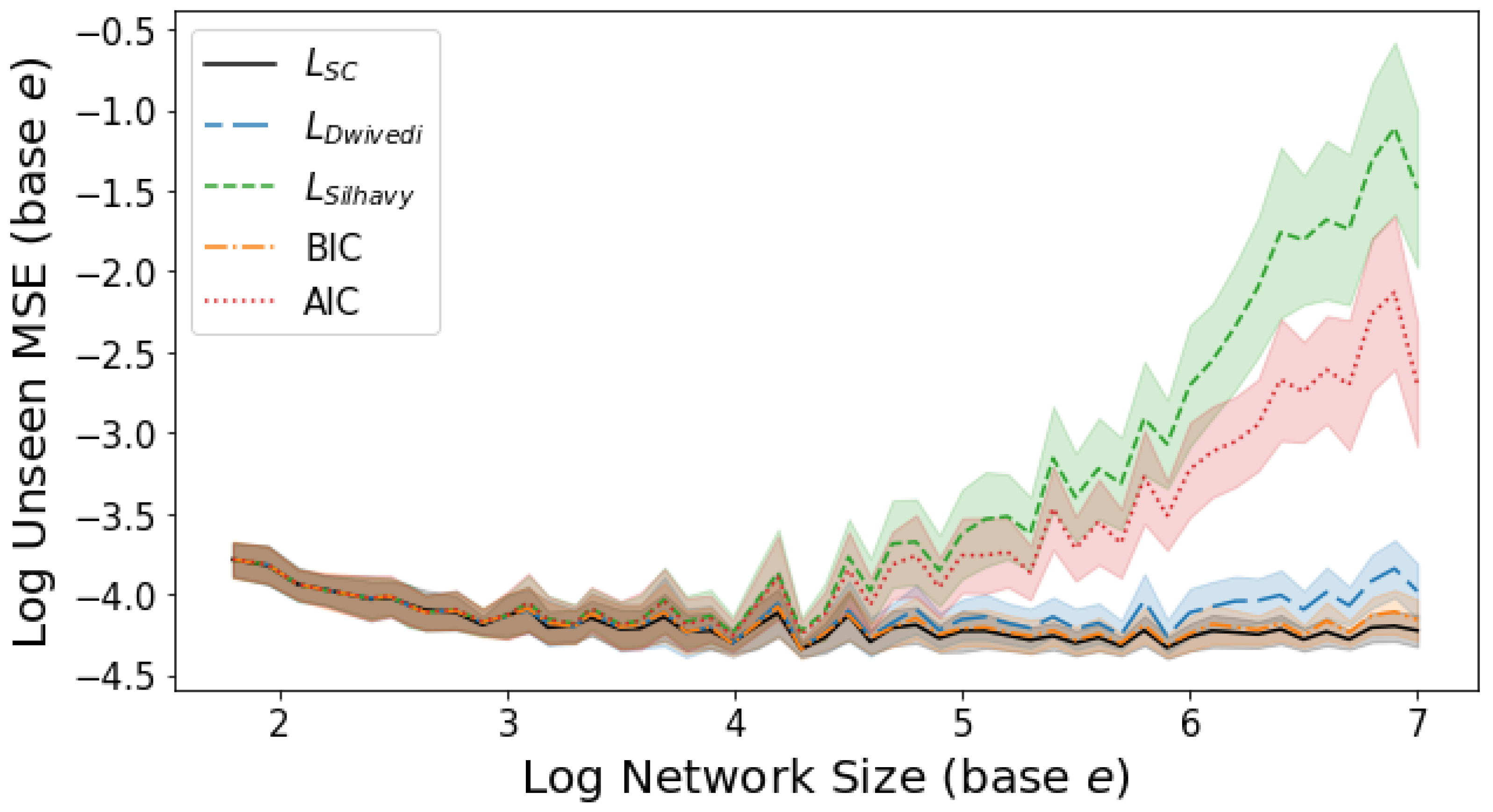
The average generalization error for one-step prediction of Lorenz-96 is compared with network size in Figure 2. The ridge penalty chosen according to stochastic complexity (in black) produces smaller generalization error on average than any fixed penalty magnitude. This is true across a range of network sizes and suggests that our method leads to sensible choices for the ridge parameter. Our criterion also achieves comparable results to some of the alternative approaches mentioned in Section 5, and performs comparatively well on large networks. This is demonstrated in Figure 3. It should be noted that the relative strength of the model complexity term is dependent on the value of $ϵ$ for these methods, which we choose to be the smaller of the two values described in Section 4

$${ϵ}^2=min({\displaystyle \frac{n{\sigma }_{Y,0}^2}{n-k}},{\displaystyle \frac{Y^T(\mathbb{I}-M_{{\alpha }^{\prime }})Y}{n-\mathrm{Tr}\left(M_{{\alpha }^{\prime }}\right)}}).$$

The first of these values is always positive and defined, since the length of the training time series is 1200 points and the largest network has 1096 nodes. The latter is calculated using a fixed value of ${\alpha }^{\prime }=\exp (-14)$, which we select because the resulting variance estimate ${ϵ}^2$ tends to be stable for perturbations around this value, and a regularization strength of $\alpha =\exp (-14)$ tends to produce well-performing echo-state network readouts.

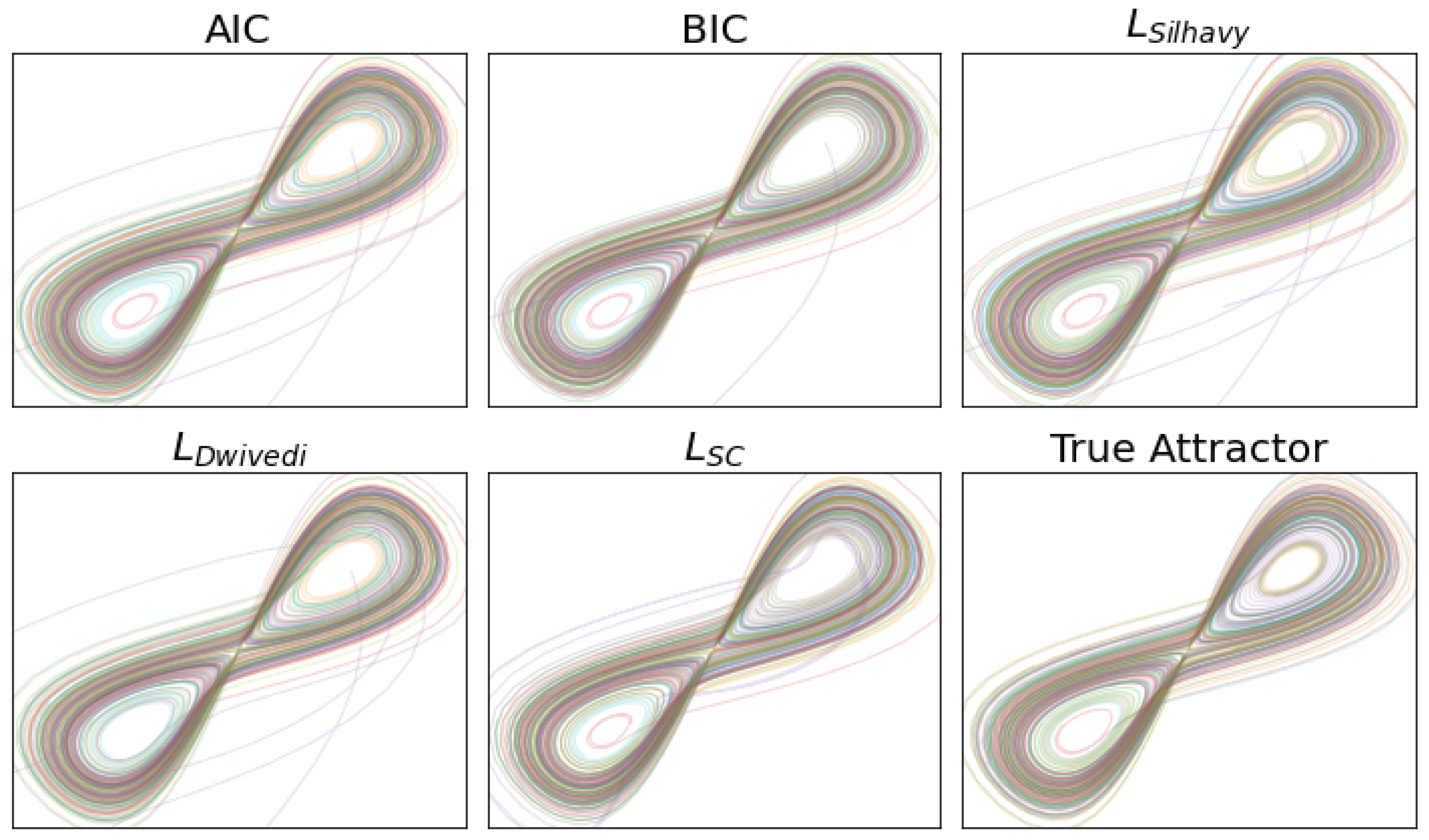
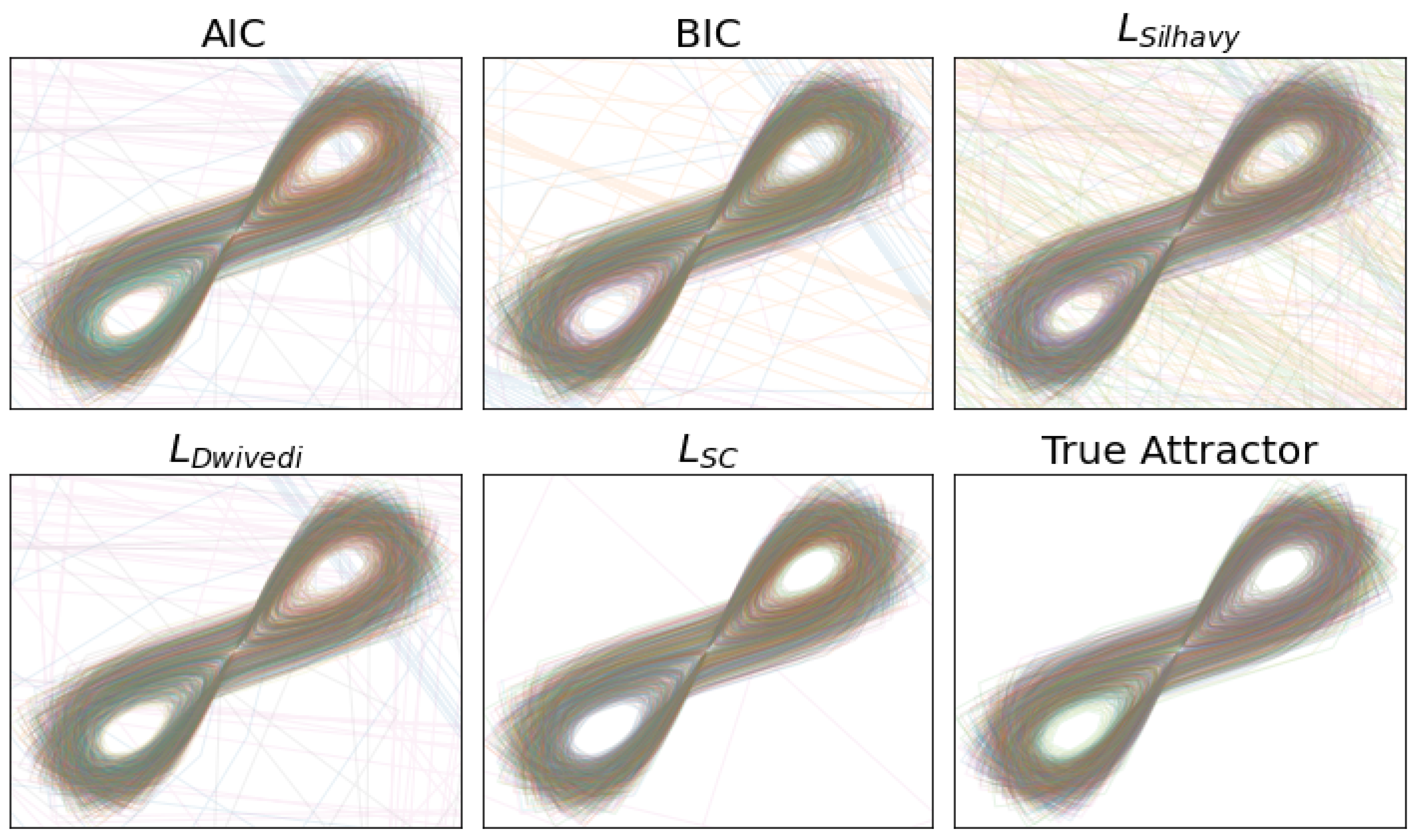
Qualitative comparisons of reconstruction ability are also provided in Figure 4 and Figure 5. This time, echo-state networks are trained for one-step-ahead prediction of the Lorenz system. Individual trajectories in each subplot are generated by continuously driving echo-state networks with their own past predictions. These predictions depend on output coefficients, which in turn depend on the ridge strength selected by each criterion. All criteria tend to produce reconstructions that are qualitatively similar to the Lorenz attractor when networks and prediction step sizes are small. This indicates that the ridge strengths they select tend to be appropriate for capturing the underlying dynamics. For example, the reconstruction composites in Figure 4 are made using 200 node networks trained at a sampling rate of $0.02$ s. On the other hand, ridge strengths selected by stochastic complexity appear to produce reasonable reconstructions more often when networks and step sizes are larger. This is the case in Figure 5, where predictions are made using 800 node networks and a step size of $0.1$ s.

8. Results on PMLB Datasets

In this section, we replicate the benchmark testing performed by Dwivedi et al. [20] on the publicly available real-world datasets from the PMLB GitHub repository [22] (v1.0.2). Of the 122 datasets in the repository that are intended for regression, we ignore those that have fewer than 5 features, and test the information theoretic criteria discussed in this paper on the remaining 109 datasets. These datasets are sourced from a wide range of research areas.

The original experiments performed by Dwivedi et al. [20] use cross-validation for benchmarking and establish that their method performs well in comparison. This is the case in particular when data are scarce. For the sake of introducing a second point of comparison, we instead perform benchmarking with Stein’s unbiased risk estimate [47,48] (SURE).

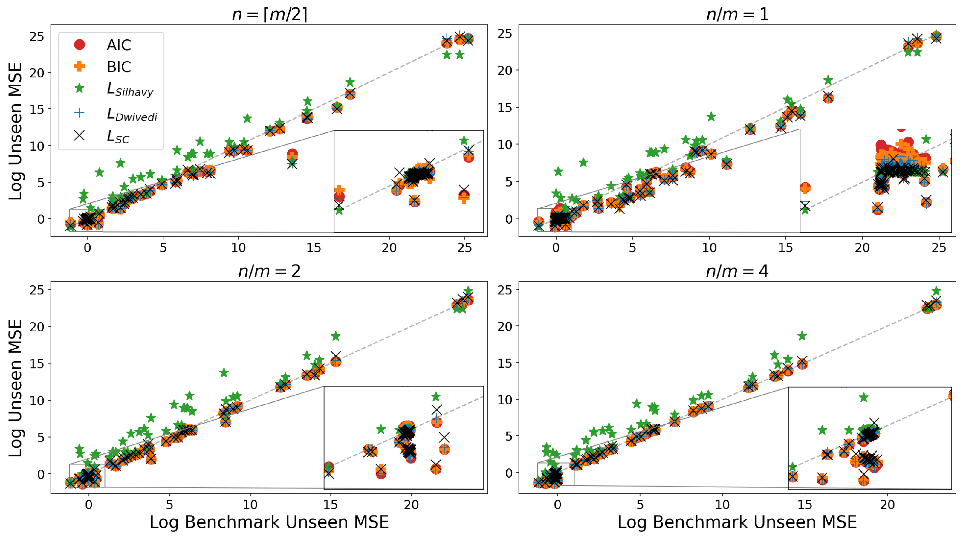
In Figure 6, we plot the average testing MSE achieved with each information theoretic criteria against the average achieved using SURE. The results in each subplot are achieved using a different ratio of training data points n to the number of dataset features m (which is also the number of tunable parameters). These ratios range from over-parameterized ($n=\lceil m/2\rceil$) to moderately parameterized ($n=4m$). In each of the 50 samples that we average across to produce the results in Figure 6, a random subset of rows is selected from each dataset for training, and the rest are reserved for testing. We estimate the variance hyper-parameter ${ϵ}^2$ using Liu’s method [28] whenever the ratio of n to m is less than one. Otherwise, like in the previous section, we take the smaller of the estimates provided by the methods discussed in Section 4. However, because the typical scale of data varies widely between datasets in the PMLB repository, we adjust the value of ${\alpha }^{\prime }$ used in Liu’s method by the average squared magnitude ${\overline{x}}^2$ of the entries in each dataset (${\alpha }^{\prime }=\exp (-14){\overline{x}}^2$).

In the highly-parameterized settings ($1/2\le n/m\le 2$) the information theoretic criteria discussed in this paper tend to perform well in comparison to the benchmark performance provided by SURE and similarly to one another. This aligns with the findings of Dwivedi et al. [20] and the comparison they drew with cross-validation. As the number of data points used for training is increased beyond the highly-parameterized settings, performances across all methods, including the benchmark, tend to become more similar.

9. Summary and Comments

We have proposed a selection criterion for the choice of penalty strength in ridge regression. In the process, we have demonstrated an application of stochastic complexity to a common problem. This required that we devise a model encoding scheme in accordance with the typical stochastic complexity scheme, but which is sensitive to the application of regularization. Our scheme suggests that we can consider the reduction in model complexity induced by regularization as a constraint on model flexibility. We believe that this result is consistent with the intuitive message espoused by stochastic complexity—that we should be hesitant in choosing a model class that fits our data well if it provides good fits to unrelated datasets using the same predictors. Regularization should ease our hesitancy by preventing our model from easily fitting these unrelated datasets.

The ridge penalty selection criterion that we derived produced promising results when used to fit linear readouts for echo-state networks. It also performed well in highly-parameterized settings on real-world datasets from the PMLB repository when compared to the benchmark provided by Stein’s unbiased risk estimate. However, this performance was well aligned with other information-theoretic criteria.