Article

Overview of Mathematical Relations Between Poincaré Plot Measures and Time and Frequency Domain Measures of Heart Rate Variability

1
Department of Vascular Medicine, University of Groningen, University Medical Center Groningen, 9700 RB Groningen, The Netherlands
2
Department of Experimental Psychology, University of Groningen, 9712 TS Groningen, The Netherlands
3
Department of Psychiatry, Interdisciplinary Center Psychopathology and Emotion regulation (ICPE), University of Groningen, University Medical Center Groningen, 9700 RB Groningen, The Netherlands
*
Author to whom correspondence should be addressed.
Entropy 2025, 27(8), 861; https://doi.org/10.3390/e27080861
Submission received: 5 June 2025 / Revised: 6 August 2025 / Accepted: 12 August 2025 / Published: 14 August 2025
(This article belongs to the Section Information Theory, Probability and Statistics)

Abstract

The Poincaré plot was introduced as a tool to analyze heart rate variations caused by arrhythmias. Later, it was applied to time series with normal beats. The plot shows the relationship between the inter-beat interval (IBI) of one beat to the next. Several parameters were developed to characterize this relationship. The short and long axis of the fitting ellipse, SD1 and SD2, respectively, their ratio, and their product are used. The difference between the IBI of a beat and m beats later are also studied, SD1(m) and SD2(m). We studied the mathematical relations between heart rate variability measures and the Poincaré measures in the time (standard deviation of IBI, SDNN, root mean square of successive differences, RMSSD) and frequency domain (power in low and high frequency band, and their ratio). We concluded that SD1 and SD2 do not provide new information compared to SDNN and RMSSD. Only the correlation coefficient r(m) provides new information for m > 1. Novel findings are that ln(SD2(m)/SD1(m)) = tanh−1(r(m)), which is an approximately normal distributed transformation of r(m), and that SD1(m) and SD2(m) can be calculated by multiplying the power spectrum by a weighing function that depends on m, revealing the relationship with spectral measures, but also the relationship between SD1(m) and SD2(m). Both lagged parameters are extremely difficult to interpret compared to low and high frequency power, which are more closely related to the functioning of the autonomic nervous system.

1. Introduction

Indices of the cardiovascular system have been studied for many purposes and in various ways, such as to predict patients’ severity or incidence of cardiovascular disorders [1], as well to investigate mechanisms associated with cognitive or psychological processes [2,3]. In particular, heart rate dynamics have led to the development of numerous methods for calculating heart rate variability (HRV). Heart rate variability refers to the variation in time intervals between heartbeats (inter-beat interval, IBI), which are regulated by the autonomic nervous system (ANS). HRV measures reflect the functioning of the ANS [1,2,3].
A landmark paper by a cardiology Task Force [1] provided a comprehensive overview of the significance and calculation of HRV measures. They categorized these measures into two groups, time and frequency domain measures.
Time domain measures that are calculated from the IBI time series are the standard deviation of the normal-to-normal interval (SDNN) and the root mean square of successive differences (RMSSD). Measures that are derived from the power density spectrum of IBI are the power in the low frequency band (LF, 0.04–0.14 Hz), power in the high frequency band (HF, 0.15–0.40 Hz), and their ratio LF/HF.
An update of the Task Force overview was made by Shaffer and Ginsberg [2], highlighting renewed interest in another approach towards HRV characterization, the Poincaré plot. This graph visualizes the relationship between the inter-beat interval of beat i (IBIi, on the x-axis) and the inter-beat interval of the next beat i + 1 (IBIi+1, on the y-axis). The Poincaré plot is used to visualize and analyze the behavior of a nonlinear dynamic system [4]. Its use is not limited to IBI time series; it can be used to analyze any time series [5,6,7,8,9].
The Poincaré plot was introduced by Woo [10] as a tool to analyze heart rate variations caused by arrhythmias. Time series with arrhythmias show a plot with several clusters (e.g., Figure 1A). Most types of arrhythmias have a distinct IBI pattern. It starts with a short interval—the ectopic beat occurs earlier than the expected normal beat, and this beat is followed by a longer interval—and the expected normal beat would start during the phase that the heart is still recovering from the ectopic beat.
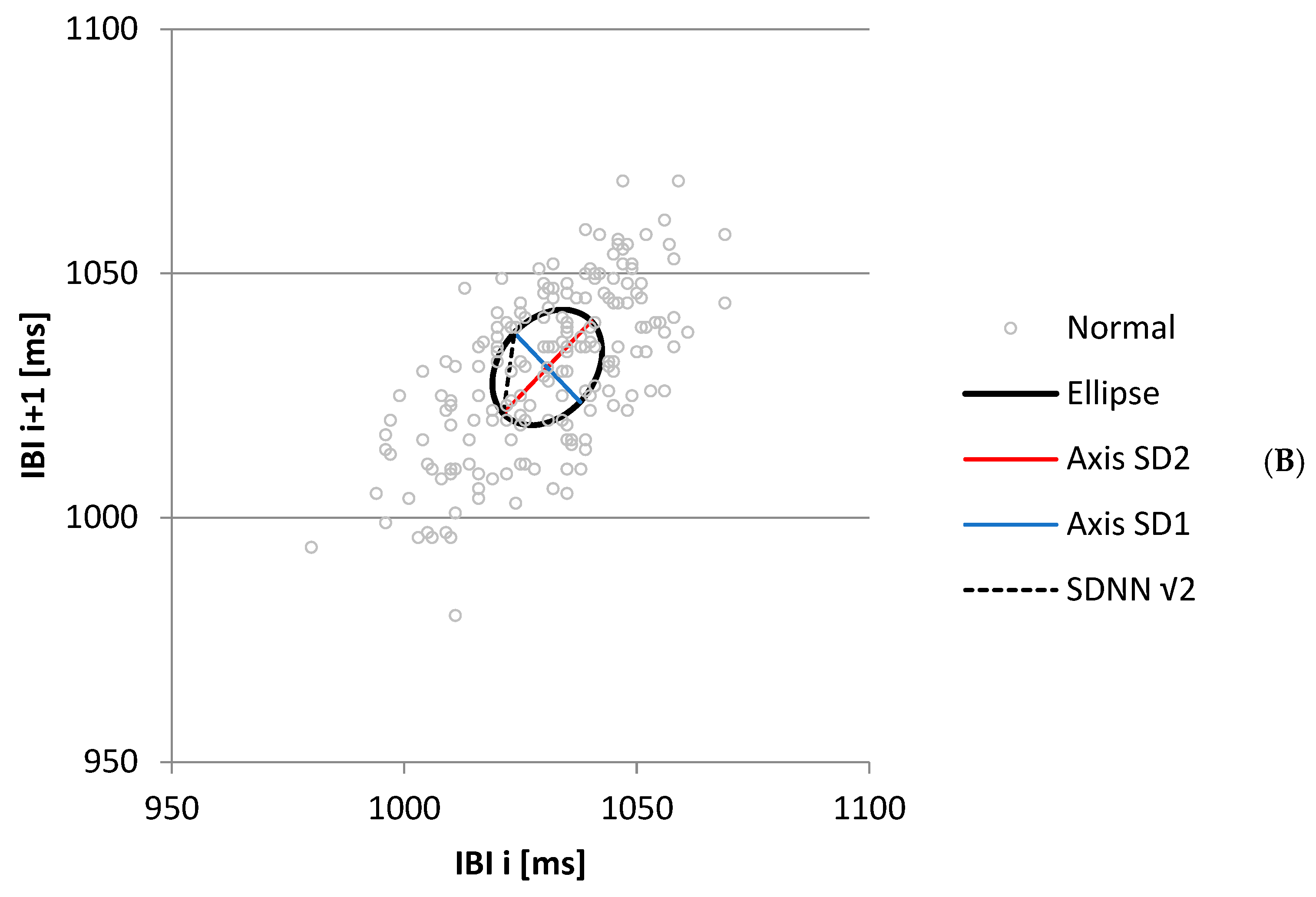
For time series with normal beats, the shape of the plot is ellipse-like. The short and long axes of the characteristic ellipse are SD1 and SD2, respectively (Figure 1B). The long axis of the ellipse coincides with the line y = x, while the middle point of the ellipse is the point with an x- and y- coordinate equal to the mean inter-beat interval. In some publications [11,12], the plot is called a Lorenz plot with a T (SD1) and L (SD2) axis. Additionally, combinations of the parameters were studied. Following the LF/HF ratio in the frequency domain, which was originally intended [2] as a parameter to reflect the balance between parasympathetic and sympathetic parts of the ANS, ratios [13,14] of SD1 and SD2, its product [15,16], which is related to the area of the ellipse, and the ratio of the standard deviation of the successive differences of IBI (SDSD) and SDNN are introduced.
During the 1990s, the physiological interpretation of SD1 and SD2 was developed with the idea that these two parameters could show different aspects of HRV than SDNN and RMSSD. However, Brennan [17] showed that this is not the case. However, this notion was not widely adopted by authors; they were still treated as independent parameters by many. For instance, several studies [12,15,18] showed a very high correlation (0.98–1.00) between SD1 and RMSSD, although sometimes the correlation dropped [12] to 0.65 during exercise with a complete parasympathetic blockade. A book on this topic [19] was published in 2013, and a reminder was published in 2017 by Ciccone [20] about the equivalence of RMSSD and SD1 and that it is not worthwhile to report them both.
Beside the differences between two successive inter-beat intervals, the difference between inter-beat interval of a beat a number m beats later, IBIi+m, and inter-beat interval is studied. The corresponding Poincaré plot is named the extended [5] or m-lagged [21] plot, with IBIi+m on the y-axis. While the parameters of lag 1 are related to fast, parasympathetic changes at larger lags, slower and longer lasting, sympathetic effects can be studied. Moreover, the relationship of the Poincaré parameters with spectral measures is studied [12,15,21], showing different correlations and interpretations. Contreras [21] studied the relationship between LF, HF, and SD1(m) for m = 1 …10. The correlation was different for the different lags and differed between healthy controls and diabetic patients.
This paper is divided into two parts. In part I—named ‘Time Domain’—we summarize Brennan’s publication [17], in which he uses the expected value function to show the relationship between the Poincaré plot parameters. We explore the mathematic relationships of SD1, SDSD, and RMSSD in full detail. The introduced ratios and area of the ellipse for different lags are evaluated, using the autocorrelation equations of Brennan as a starting point.
In part II—named ‘Frequency Domain’—we investigate how the Poincaré parameters are related to the distribution of power in the spectrum. We investigate the relationship between m-lagged parameters SD1(m) and SD2(m) and the power density spectrum in the second part. We approach the m-lag Poincaré plot as a filtering process of the IBI time series. This will reveal the close relationship with the power density spectrum of IBI and the m-lagged Poincaré measures.
In this manuscript, we focus on the mathematical relationships between the IBI measures and extend the calculations to m-lagged derived parameters, giving a comprehensive overview of the Poincaré plot analysis in the time and frequency domain. Moreover, the results can be used for other time series as well.

2. Materials and Methods

We summarized the symbols used and their definitions in the abbreviation section.

2.1. Tools for Part I: Time Domain

In this methods section, we give an overview of some basic mathematics that we need to derive the relationships described by Brennan [17] and new relationships for the derived measures, such as SD1/SD2. We use the expected value of a time series variable x(t), having N equidistant samples xi at ti, which is defined as follows [17,22]:
E x ( t ) = 1 N i = 1 N x i = x ¯
with basic rule E[x + y] = E[x] + E[y]. The variance of x(t) is shown as follows [17,22]:
E x t x ¯ 2 = E x 2 t   x ¯ 2
The autocorrelation R(τ) for a time series x(t) is shown as follows [17,22]:
R τ = E x t E [ x t ] x t + τ E [ x t + τ ]
and for a stationary time series, E x t = E x t + τ = x ¯ [22]. R(τ) is then found with the following equation [17]:
R τ = E x t x t + τ x ¯ 2

2.2. Tools for Part II: Frequency Domain

In the frequency domain analysis, we show that SD1(m) and SD2(m) can be calculated as the output of a filter applied to the IBI time series. For this filter approach, we use the following basic summation rule for integration:
f x + g x   d x = f x   d x + g x   d x
The autocorrelation function is the inverse Fourier transform of the power density spectrum, also known as the Wiener–Khinchine relation [22,23]. For single-sided power density spectra of IBI, PIBI(f), the relation is shown as follows [22]:
R τ = 0 P I B I f cos 2 π f τ d f
With these tools, we establish the relationships between the indices mathematically.

3. Results

3.1. Part I: Time Domain

3.1.1. The Expected Value Approach (Brennan’s Findings)

In this section, we summarize the findings of Brennan [17]. The time series of inter-beat intervals IBI is used to calculate the time series of successive differences (SD). Usually, the differences with the next beat are calculated, but larger beat lags are also used. We refer to this time series as successive differences with a lag of m beats, as follows:
S D i m = I B I i + m I B I i
We calculate the statistics for N inter-beat intervals, and thus N − 1 successive intervals, but assume that N + m inter-beat intervals are available. For large N and a stationary IBI time series, the mean of the successive differences will be very close to zero (this is explained in the next section in detail). The mean and standard deviation can be defined by the following expected value function:
I B I ¯ = E I B I i  
S D ( m ) ¯ = E S D i m 0
S D N N 2 = E I B I i 2 I B I ¯ 2
S D S D 2 m = E S D i 2 m S D ( m ) ¯ 2 E [ S D i 2 m ]
and by the following definition:
R M S S D 2 = E [ S D i 2 1 ]
The autocorrelation or autocovariance function between the IBI time series and the m-lagged time series is shown as follows:
R m = E I B I i + m I B I ¯ I B I i I B I ¯ = E I B I i + m I B I i I B I ¯ 2
Clearly, when m = 0, Equation (13) is equal to (10), so the following is true:
S D N N 2 = R ( 0 )
Now, for a stationary IBI time series, we can express SDSD2(m) as a difference of two autocorrelations, as follows:
S D S D 2 m = E I B I i + m I B I i 2 = E I B I i + m 2 I B I ¯ 2 2 E I B I i + m I B I i + 2 I B I ¯ 2 + E I B I i 2 I B I ¯ 2 = 2 ( R ( 0 ) R ( m ) )
The Pearson correlation coefficient for lag m is shown as follows [17,22]:
r m = E [ I B I i + m I B I ¯ I B I i I B I ¯ ] E [ I B I i + m I B I ¯ 2 ] E [ I B I i I B I ¯ 2 ] = R ( m ) R ( 0 )
Brennan [17] showed that the short and long axes of the ellipse in the lag m Poincaré plot can be found as follows:
S D 1 2 m = R 0 R m = 1 2 S D S D 2 m
S D 2 2 m = R 0 + R m = 2 S D N N 2 1 2 S D S D 2 ( m )
SD1(m) is the standard deviation of the time series SD1i(m), as defined in Equation (7), divided by 2. Therefore, the sum of SD12(m) and SD22(m) can be found as follows:
S D 1 2 m + S D 2 2 m = 2 R 0 = 2 S D N N 2
This means that, for all m, SD1 or SD2 is sufficient to report if SDNN is reported. The geometric representation of Equation (19) is that SDNN √2 is equal to the hypotenuse of a right triangle with sides SD1(m) and SD2(m). This is indicated in Figure 1B for m = 1. If R(m) becomes zero, and thus the correlation r(m) = 0, we find the following to be true:
r m = 0 S D 1 m = S D 2 m = S D N N

3.1.2. Relation RMSSD, SDSD, and SD1

As shown in the previous section, the differences between RMSSD, SDSD, and SD1 are only small. We show the precise relationships in this section for the ‘original’ successive differences (m = 1), in order to show under which conditions the trio can be considered to be identical. The N inter-beat intervals result in N − 1 successive differences with mean, and the equation is shown as follows:
S D ¯ = 1 N 1 i = 1 N 1 S D i = 1 N 1 i = 1 N 1 I B I i + 1 i = 1 N 1 I B I i = 1 N 1 i = 2 N I B I i i = 1 N 1 I B I i
We make the summation range equal for both summations, but we have to subtract the extra values as follows:
S D ¯ = 1 N 1 i = 1 N I B I i I B I 1   i = 1 N I B I i I B I N = I B I N I B I 1 N 1
For large N and/or small difference between the first and last inter-beat interval, the mean of SD will be close to zero. If a time series is stationary, assumed for all time domain and spectral measures, the difference between the first and last beat will indeed be small. Now, the squared parameters are shown as follows:
R M S S D 2 = 1 N 1 i = 1 N 1 S D i 2 = S D S D 2 + S D ¯ 2 2 S D 1 2 + S D ¯ 2
S D S D 2 = 1 N 1 i = 1 N 1 S D i S D ¯ 2 = R M S S D 2 S D ¯ 2 2 S D 1 2
S D 1 2 = 1 N 1 i = 1 N 1 S D i S D ¯ 2 2 = 1 2 R M S S D 2 S D ¯ 2 1 2 S D S D 2
Note that we divided the sum by N − 1 instead of N − 2 for SDSD and SD1, which corresponds with the expected value approach of Brennan [17]. When S D ¯ 0 , then this reduces to the following:
R M S S D 2 = S D S D 2 = 2 S D 1 2
For stationary IBI time series of normal beats with sufficient length (usually 5 min or more), this is valid.

3.1.3. Derived Measures SD1/SD2, SDSD/SDNN, and Ellipse Area

A number of measures are derived from the time domain measures and SD1 and SD2, including the ratio of SD1 and SD2 (and of SD2 and SD1), the ratio SDSD/SDNN, and the area of the ellipse. The rationale for the use of ratios is the same as for LF/HF in the frequency domain. However, now aware of the relationship between SD1, SD2, SDSD, and SDNN, the relationship between the derived measures can be explored, not only for lag m = 1, but for any lag. We start with the most commonly used ratios, SD1/SD2 and SD2/SD1, as follows:
S D 1 2 ( m ) S D 2 2 ( m ) = R 0 R ( m ) R 0 + R ( m ) = 1 R ( m ) / R ( 0 ) 1 + R ( m ) / R ( 0 ) = 1 r ( m ) 1 + r ( m )
So,
S D 1 ( m ) S D 2 ( m ) = 1 r ( m ) 1 + r m   a n d   S D 2 ( m ) S D 1 ( m ) = 1 + r ( m ) 1 r ( m )
For r(m) values that are close to zero, (|r(m)| < 0.15), the ratio SD1/SD2 can be approximated by the following:
S D 1 ( m ) S D 2 ( m ) = 1 r ( m ) 1 + r m   1 r ( m ) 1 r m = 1 r m 1 1 r 2 m 1 r ( m )
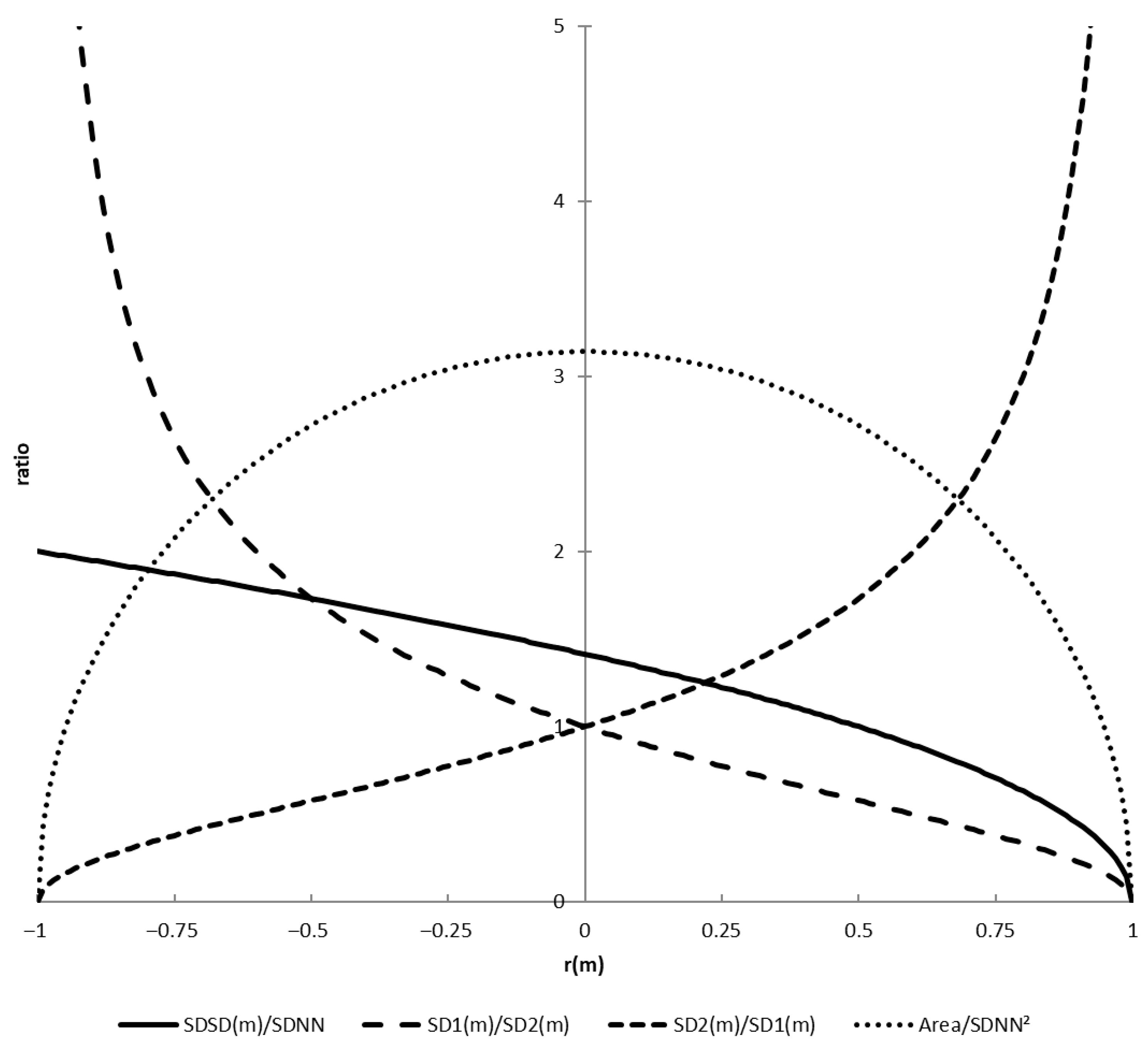
The ratios only depend on the correlation between the original and lagged IBI series. This relationship was already shown by Carrasco [12] for Lorenz plots (in Figure 2 of Carrasco, L/T = SD2(1)/SD1(1) is shown in relation to positive r(m) values). Interestingly, the natural logarithm of SD2/SD1 is commonly used as a normal distributed transformation of correlations coefficients, shown as follows [12,24,25]:
z ( m ) = l n S D 2 m S D 1 m = l n 1 + r m 1 r m = 1 2 l n 1 + r m 1 r m = t a n h 1 ( r m )
Tanh−1(x) is the inverse hyperbolic tangent function. Note that the range of this function is from −∞ (for r(m) = −1) to +∞ for (r(m) = 1) and that, if the value z(m) = c for r(m), then z(m) = −c for −r(m). Since z(m) and SD2(m)/SD1(m) are strictly monotonic increasing functions of r(m), the inverse functions exist, and the interpretations of z(m), SD2/SD1, and r(m) are identical. Taking the natural logarithm of SD1/SD2 but with a minus sign gives the same result.
  • For the ratio SDSD/SDNN, we find the following:
S D S D 2 ( m ) S D N N 2 = 2 ( R 0 R m ) R ( 0 ) = 2 1 R m R 0 = 2 1 r m
Hence, the following can be found:
S D S D ( m ) S D N N = 2 1 r m
Rearranging (32) gives an easy way to calculate the correlation r(m), as follows:
r m = 1 1 2 S D S D 2 ( m ) S D N N 2
In Figure 2, the relationship between the ratios and r(m) is shown. Note that r(m) is a correlation coefficient and limited to the range −1 to 1. Because of this, the ratio SDSD(m)/SDNN is limited to the range 0 to 2 (and also the ratio RMSSD/SDNN is approximately limited to this range).
The last derived measure to explore is the area of the ellipse in the Poincaré plot. The area of an ellipse is the product of both axes multiplied by π. The squared product of SD1(m) and SD2(m) is shown as follows:
S D 1 2 m S D 2 2 m = R 0 R m R 0 + R m = R 2 0 R 2 m = R 2 ( 0 ) 1 R 2 ( m ) R 2 ( 0 )
The area is now the following:
π   S D 1 m   S D 2 m = π   R 0 1 R ( m ) R ( 0 ) 2 = π   S D N N 2 1 r 2 m
The area values can range from 0 to π SDNN2. For time series with r2(m) ≈ 0.9, the area is equal to SDNN2. The ratio of the area and SDNN2 and r(m) is also shown in Figure 2. We have shown that all derived parameters are related to one new parameter, which is r(m). Reporting the correlation at lag m is therefore sufficient.

3.2. Part II: Frequency Domain

So far, we have evaluated the time domain measures. To explore the frequency domain, we assume that SD12(m) or SD22(m) is the total power of the output of a filter with the IBI time series as input. Applying a filter means, in the spectral domain, that you multiply the spectral values with certain weighing factors. An example is shown in Appendix A for the calculation of the power in the low frequency band LF. The filter characteristics determine the values of the weighing factors. In this section, we show which weighing factors must be used for a filter that has SD12(m) and SD22(m) as total power of the filter output. The filter characteristic H(f), the transfer function, of such a filter to calculate SD1(m) or SD2(m) must be determined.
The autocorrelation function is found as follows, using the Wiener–Khinchine relation (6), for lag m:
R m = 0 P I B I f cos 2 π f m I B I ¯ / 1000 d f
We have to include m multiplied by I B I ¯ / 1000 to create an average time lag τ in seconds, instead of the lag in number of beats, in the cosine argument. Note that Parseval’s theorem is a special case of the Wiener–Khinchine relation (6); for m = 0, the cosine argument is always 0 and cos(0) = 1. For the correlation, we find the following:
r m =   R ( m ) R ( 0 ) = 0 P I B I f cos 2 π f m I B I ¯ / 1000 d f 0 P I B I f   d f
This relationship can be helpful to explain findings where a specific spectral shape is assumed, like in the simulations performed by Satti [5]. In Appendix B, we show this in detail. In Appendix C, we show an alternative approach to calculate the transfer function, which is more direct but requires knowledge of the mathematics of complex numbers.
Now, we start with SD1(m), combining Equations (17), (36), and (5) as follows:
S D 1 2 m = R 0 R m = 0 P I B I f d f 0 P I B I f cos 2 π f m I B I ¯ / 1000 d f = 0 ( 1 cos 2 π f m I B I ¯ / 1000 )   P I B I f d f
For SD1(m) squared, the transfer function is shown as follows:
H S D 1 ( m ) f 2 = 1 c o s ( 2 π f m I B I ¯ / 1000 )
For SD2(m), the only difference is the minus sign, shown as follows:
H S D 2 ( m ) f 2 = 1 + c o s ( 2 π f m I B I ¯ / 1000 )
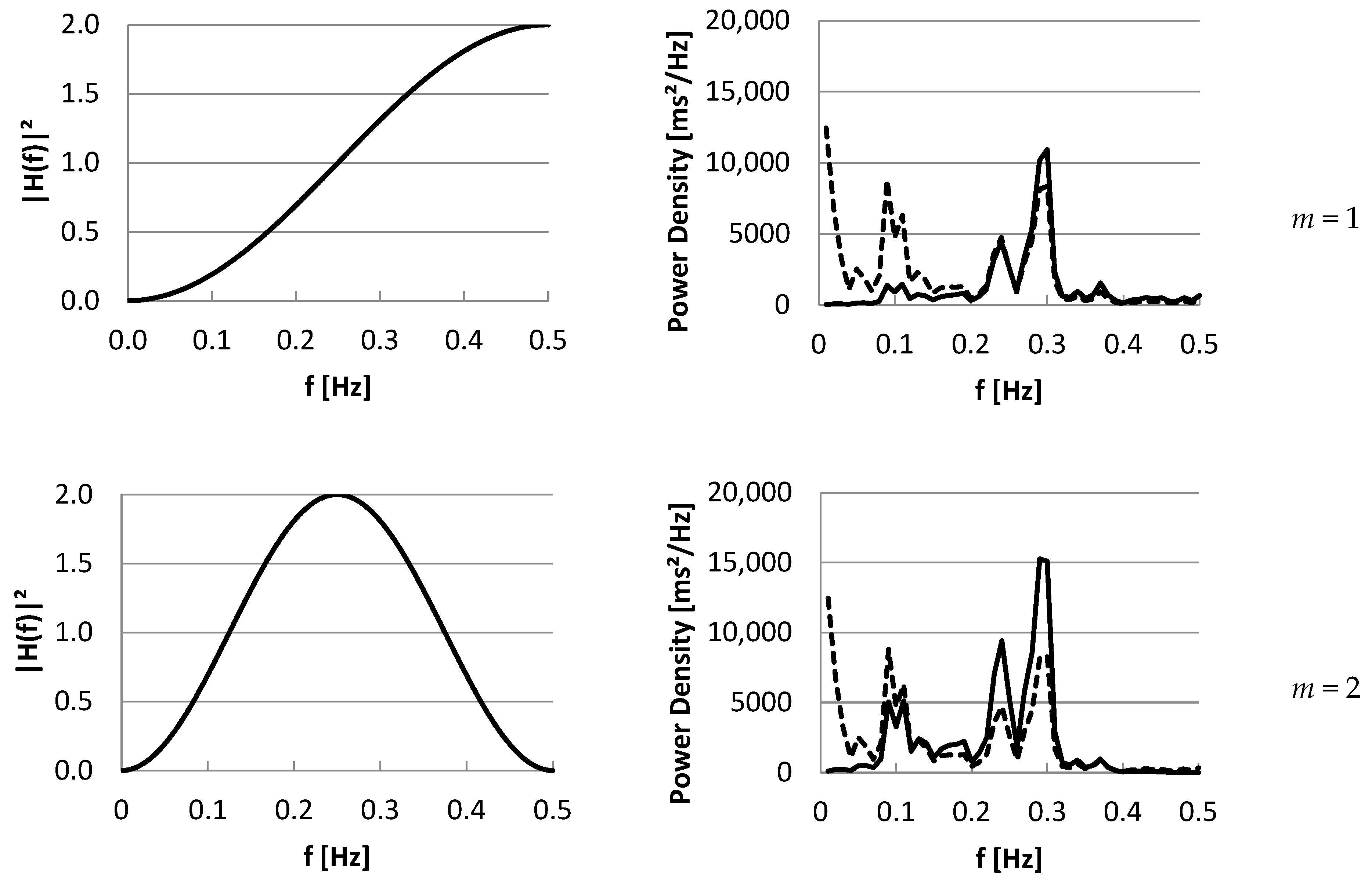
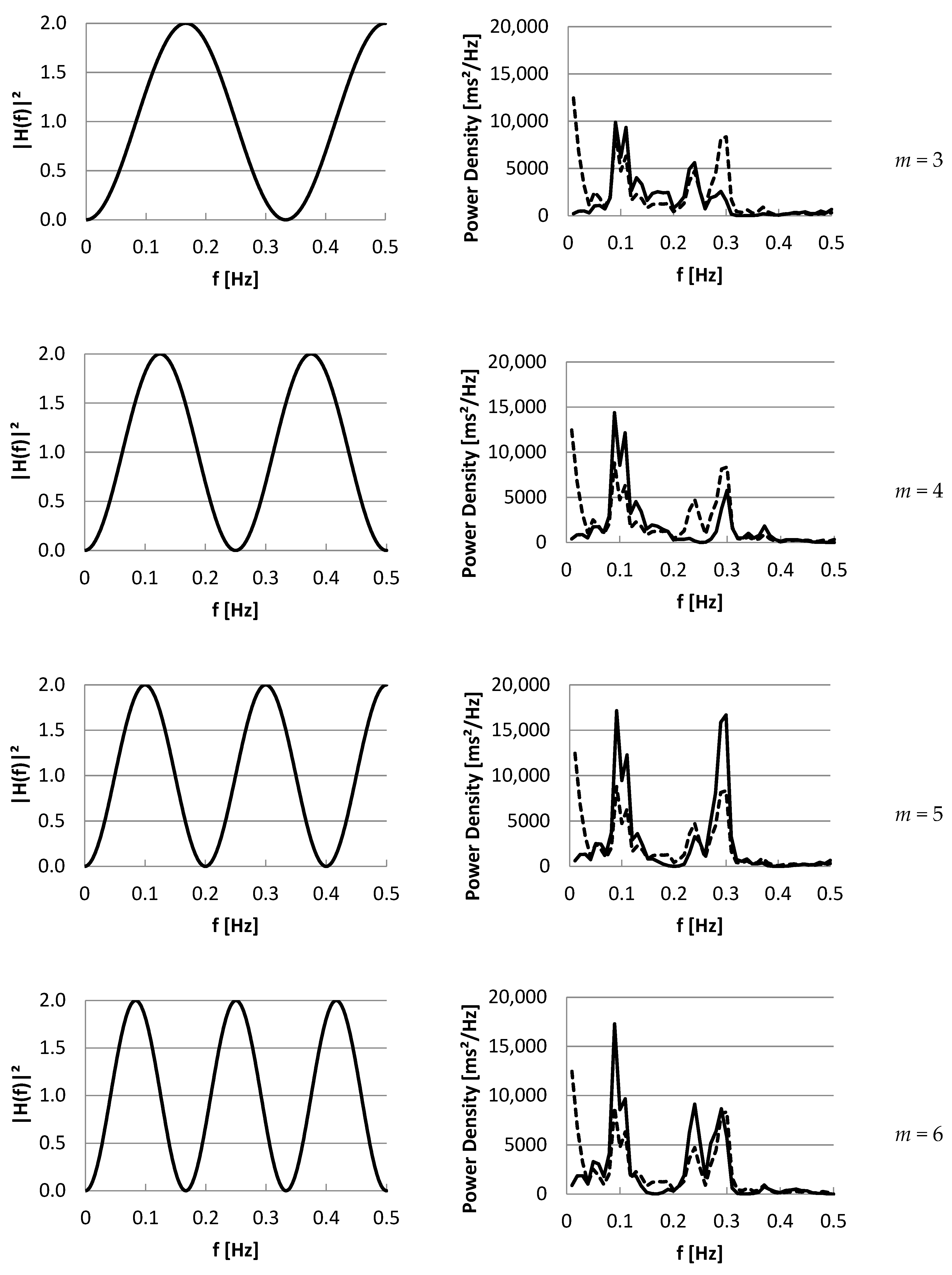
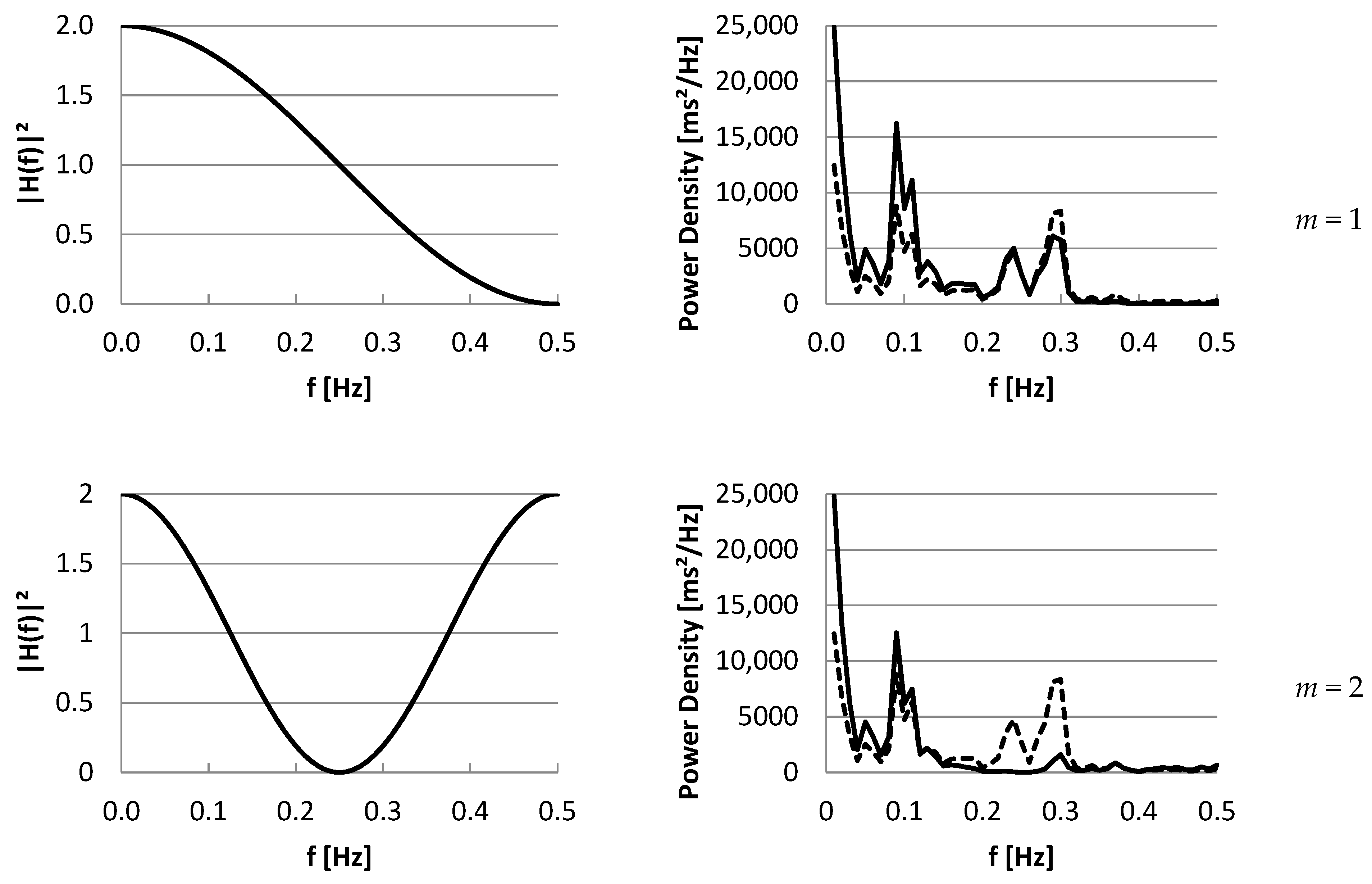
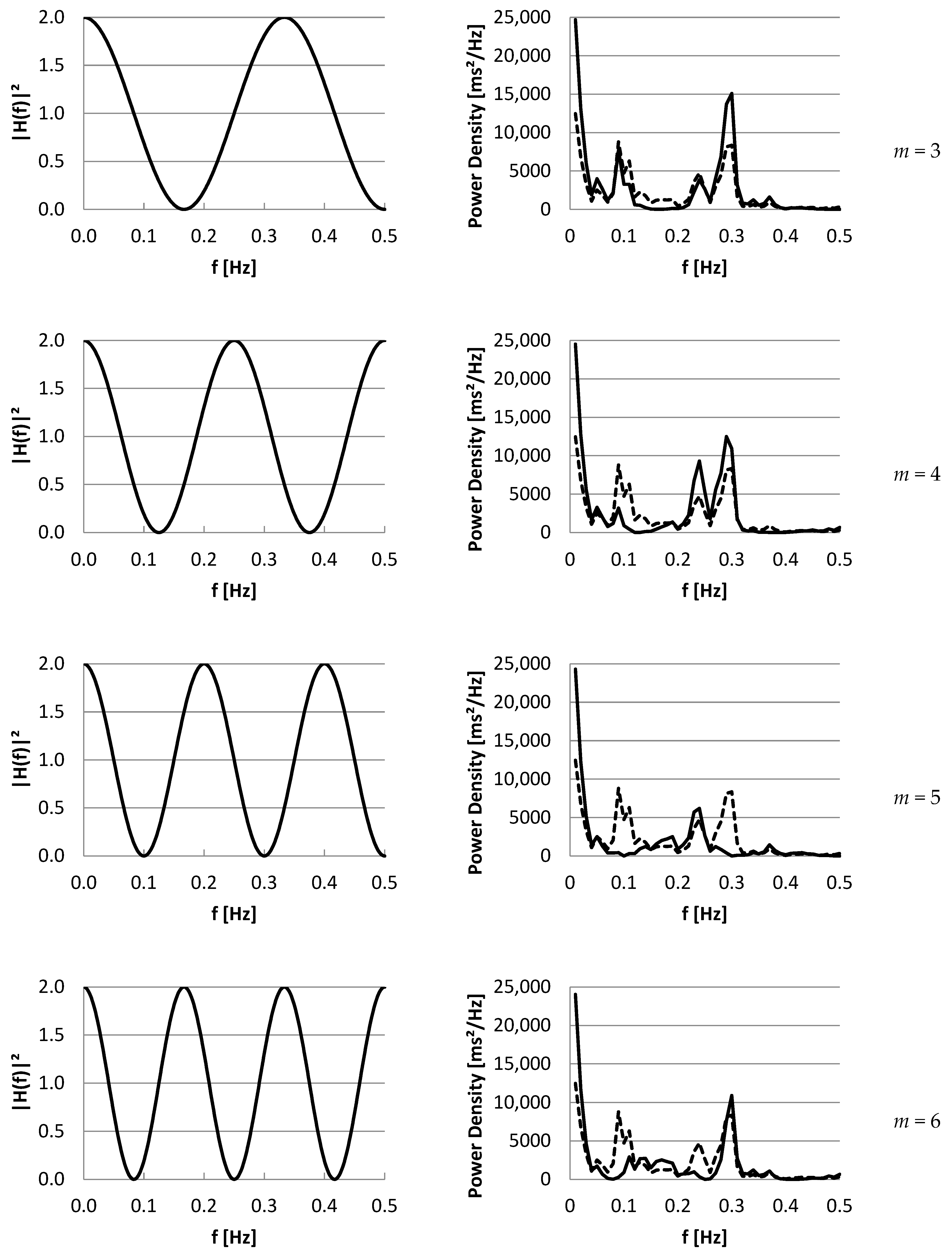
In Figure 3, we show the squared transfer functions for SD1(m), at lags m = 1 …6 and 10, in case mean IBI is 1000 ms, in the left panel. In the right panel, an example of IBI power density spectrum is shown (dashed). Multiplying the IBI power spectrum by the squared transfer function for each frequency, as described in Equation (38), results in the spectrum of SDi(m) (solid). The area under this spectrum equals the total power, which is SD12(m). In Figure 4, the same panels for SD2(m) are shown. In the Supplementary Materials, an Excel sheet is available to create these figures for other I B I ¯ and m values.
Note that, for RMSSD, the transfer function of SD1(1) can be used, multiplied by 2. In the example, at lag m = 5, the power of LF + HF will be close to SD12(5). Increasing the lag to very high values will result in resampling the power density spectrum at a high frequency (m/2 samples). SD1(m) and SD2(m) will converge to SDNN; although, they will still include complementary frequencies. The ratio SD1/(m)/SD2(m) will converge to 1, corresponding with r(m) converging to 0, which makes sense, given the large lag between the beats and a non-stationary recording becoming more likely.

4. Discussion

We evaluated the mathematical relationships between time domain HRV measures SDNN and RMSSD and a series of Poincaré parameters, SD1, SD2, SDSD, their ratios, and their product, for different time lags. Like others [17,19,20], we show the great overlap between the time domain and Poincaré measures. We show that the correlation r(m) is the only parameter that adds new information to the time domain parameters for m > 1, which is also introduced in this way by Satti [5]. It is not surprising, since the Poincaré plot is in fact an analysis of the autocorrelation between the IBI time series and its m beats lagged time series. Usually [2], SD1 and SD2 are referred to as non-linear parameters, but the parameters are clearly of the same type as SDNN and RMSSD [4,17].
For larger values of m, the correlation between beat i and i + m becomes smaller. In that case, SD1(m) ≈ SD2(m) ≈ SDNN. Empirical data confirming this can be found in Figure 1 of Koichubekov [26] (left panel). At higher values of m, the SD1(m)/SD2(m) ratio is about 0.9 (right panel), which means that the correlation r(m) ≈ 0.1, using the approximation of SD1(m)/SD2(m) 1 − r(m). The ratio is often interpreted in the same way as LF/HF, and Guzik [15] shows a significant correlation between them. However, the interpretation of Stein [27], that it “captures the randomness of R-R-intervals”, is closer to what the ratio is, as −ln(SD1(m)/SD2(m)) is a normal distributed transformation of r(m). However, how can we explain the high correlation between SD2/SD1 (m = 1) and LF/HF that Guzik [15] found? Note that SD2/SD1 and r(1) are highly correlated (see Figure 2, over the range r(1) = 0.5 …0.8, R2 = 0.99) and that, for r(1), the spectral computation is found as follows:
r 1 = 1 S D N N 2 0 P I B I f cos 2 π f   I B I ¯ / 1000 d f
For frequencies up to 0.25 Hz at mean IBI = 1000 ms (=1/4 1000 / I B I ¯ ) the contribution of the power to r(1) is positive, but for higher frequencies, it is negative. Therefore, the major part of the HF power will reduce r(1), while r(1) will increase with increasing LF power. The power of LF and HF affects the ratio LF/HF in the same way, explaining their correlation.
Because of the close relationship between the Power Density Spectrum and the autocorrelation function R(m), by inverse Fourier transform, we could show the relationship between the m lagged parameters and the spectrum. Using a filter approach, we could determine the relationship between a given spectrum and the time domain and Poincaré parameters. The filter characteristic (squared modulus function) is determined by the lag m and the mean inter-beat interval of the time series. From this approach, we also know that SD12 is closely related to HF, which affects the correlation between the ratios SD2/SD1 and LF/HF. SD22 is mostly related to VLF and LF and can be used as an estimate for low frequency variability. However, while the frequency bands VLF, LF, and HF are independent, SD12 and SD22 are dependent parameters because of the overlap of their transfer functions shown in Figure 3 and Figure 4, in the range 0.15–0.30 Hz. Due to use of a lag expressed in beats, this range varies with mean IBI.
We limited our analysis to SD1, SD2, and a number of derived parameters and did not try to give a review of all publications on the subject, as they are so numerous. Of course, many other approaches used to quantify the visual and temporal aspects of Poincaré plots have been developed [19,28,29,30]. We think our findings can be helpful to determine whether (newly) developed measures provide new and independent information.

5. Conclusions

Applying the Poincaré plot for the detection and classification of ectopic beats, its intended use [10], is not questioned. However, for the analysis of normal heart rate variability, Poincaré plot measures at lag m = 1, SD1, and SD2 do not provide new information compared to SDNN and RMSSD.
We derived that ln(SD2(m)/SD1(m)) = −ln(SD1(m)/SD2(m)) is a normal distributed variable that can be used for statistical tests of the correlation coefficient r(m) and calculate confidence intervals for r(m). SD1(m) and SD2(m) are, in fact, frequency domain power measures with varying frequency bands. They can be calculated as the total power of the subjects power density spectrum after multiplying the appropriate transfer function for the desired lag. SD12(1) as well as RMSSD2 are closely related to HF.
It is important to realize that the lagged parameters depend on mean IBI and the exact spectral density of a subject (most important here is the actual respiratory frequency), resulting in a weighing of the power density spectrum differently for each subject. SD2(m) is complementary to SD1(m) at any lag because their squared values always add up to 2 SDNN2. Both lagged parameters are extremely difficult to interpret compared to LF and HF powers, which are closer related to the functioning of the ANS.
All investigated Poincaré variables, SD1(m), SD2(m), SD2(m)/SD1(m), SD1(m)/SD2(m), π × SD1(m) × SD(2(m), and SDSD(m)/SDNN, are related to r(m). Reporting r(m) is sufficient to provide new information besides SDNN.

Supplementary Materials

The following supporting information can be downloaded at: https://www.mdpi.com/article/10.3390/e27080861/s1, File S1: Excel sheets with calculations and figures.

Author Contributions

Methodology, A.M.v.R.; Formal analysis, A.M.v.R.; Writing—original draft, A.M.v.R.; Writing—review & editing, M.M.S. and J.D.L.; Supervision, H.R. All authors have read and agreed to the published version of the manuscript.

Funding

This research received no external funding.

Data Availability Statement

Data are contained within the article.

Conflicts of Interest

The authors declare no conflict of interest.

Abbreviations

The following abbreviations are used in this manuscript:
Symbol/AbbreviationDescriptionUnit
General
x ¯ Mean of xunit of x
E [ x ] Expected value of variable xunit of x
FFrequencyHz
IBeat number-
IBIiInter-beat interval of beat ims
NNumber of inter-beat intervals-
Time domain measures
I B I ¯ Mean inter-beat intervalms
RMSSDRoot mean square of successive differencesms
SDNNStandard deviation of normal-to-normal intervals, or the IBI time seriesms
Frequency domain measures
LFPower in the low frequency band (0.04–0.15 Hz)ms2
HFPower in the high frequency band (0.15–0.40 Hz)ms2
H(f)Transfer function of a filter of the IBI time series-
Px(f)Single sided power density spectrum of x(unit of x)2/Hz
VLFPower in the very low frequency (0.01–0.04 Hz)ms2
Poincaré measures
m”Time” lag expressed as number of beats-
τTime lags
r(m)Pearson correlation coefficient between IBIi and IBIi+m-
R ( m ) Autocorrelation or autocovariance function of IBIi and IBIi+mms2
SD1Short axis of the ellipse in the Poincaré plot at lag m = 1ms
SD1(m)Short axis of the ellipse in the Poincaré plot at lag mms
SD2Long axis of the ellipse in the Poincaré plot at lag m = 1ms
SD2(m)Long axis of the ellipse in the Poincaré plot at lag mms
SDiSuccessive difference of beat i and beat i + 1ms
SDi(m)Difference of IBI of beat i and i + mms
SDSDStandard deviation of successive differences, the SD time series at lag m = 1ms
SDSD(m)Standard deviation of successive differences, the SD time series at lag mms

Appendix A

The squared standard deviation of a time series is equal to the total power (area under curve) of the power density spectrum. This theorem is known as Parseval’s theorem [12]. For example, if PIBI(f) is the power density spectrum of the IBI times series, then the following is found:
S D N N 2 = 0 P I B I f d f
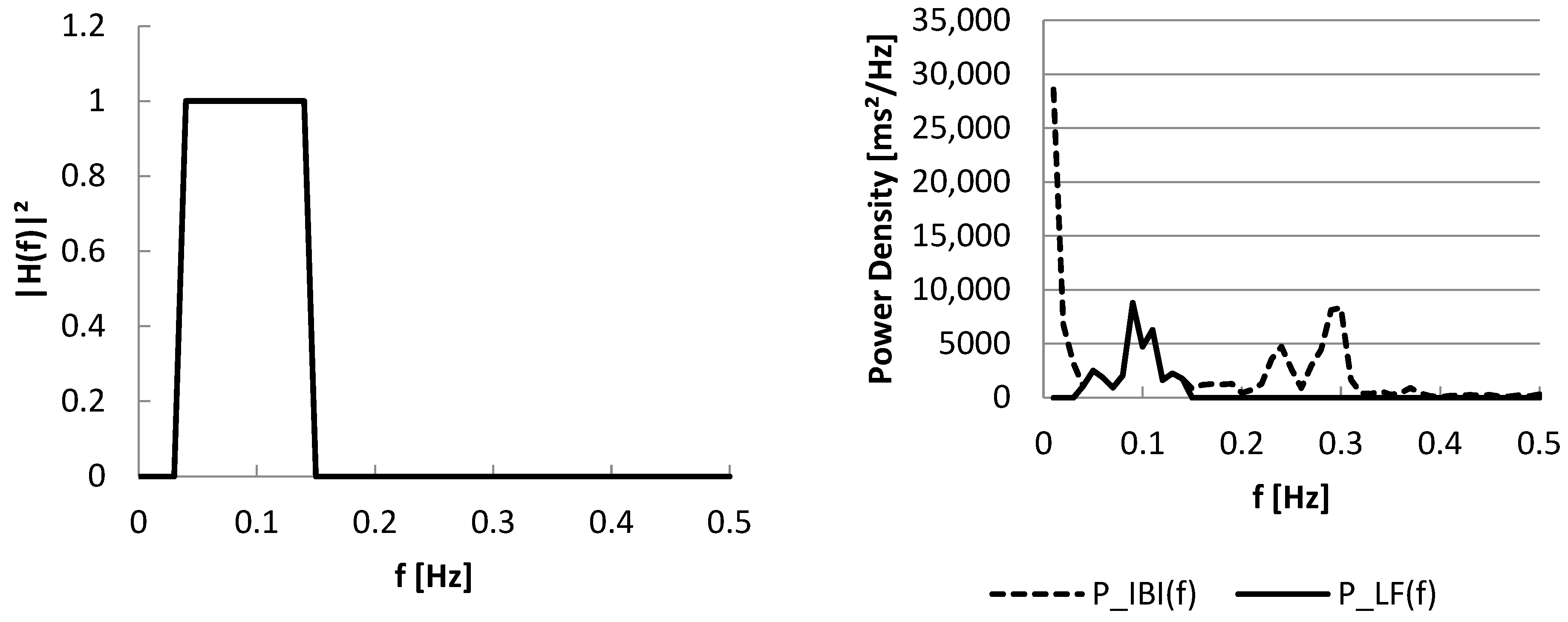
A simple example of filtering is the LF (or HF) power. LF can be assumed to be the total power of the output of a filter, with the following transfer function:
H L F f = 0                     f   o t h e r w i s e   1         0.04 f < 0.15
The power density spectrum of the output of the filter can be calculated by [22] as follows:
P L F f = H L F f 2   P I B I f
The total power of this spectrum is shown as follows:
L F = 0 P L F f d f = 0 H L F f 2   P I B I f   d f = 0.04 0.15 P I B I f d f
Figure A1 shows the squared transfer function in the left panel and the spectra of IBI and the filter output in the right panel.
Figure A1. Transfer function (left panel) for the calculation of LF power as total power of the spectrum (right panel) of a filtered IBI series.
Entropy 27 00861 g0a1

Appendix B

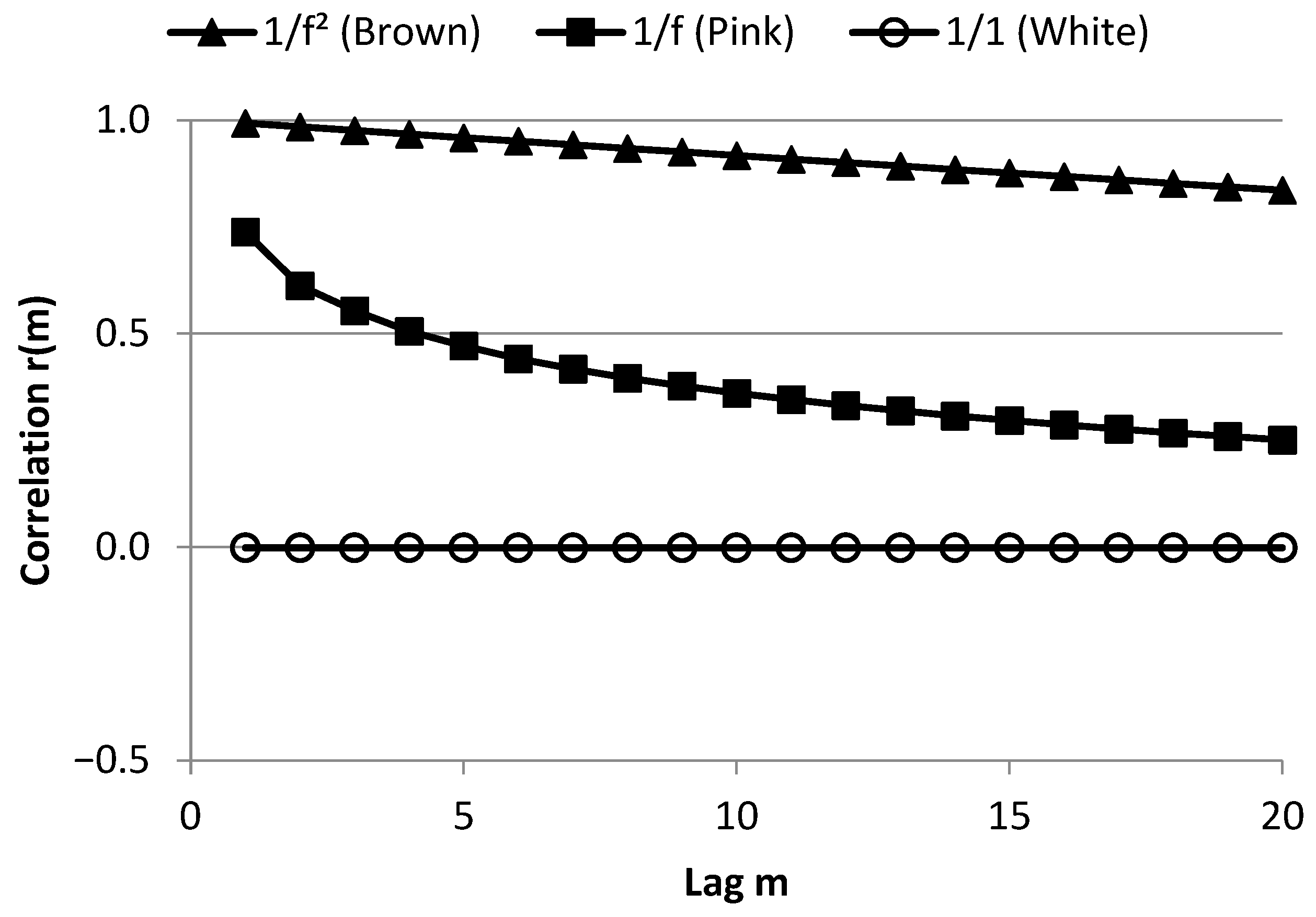
Satti [5] performed a simulation study in which the m-lagged correlations r(m) were investigated for the following three different types of noise: white, pink and brown. The spectral density spectra of these types of noise are PWhite(f) = c, PPink(f) = c/f, and PBrown(f) = c/f2. Using the Matlab random generator, they created time series of 1000 samples (personal communication with A. Mani, last author of [5]) with these properties and calculated r(m) for m=1 20. Our approach is in the spectral domain. We created spectra with these shapes, at 0.001 Hz frequency resolution (corresponding with 1000 samples), in Microsoft Excel and calculated the correlations according to the following:
r m = 0 P N o i s e f cos 2 π f m d f 0 P N o i s e f   d f
The numerical integration method used is the trapezoidal rule, integrating from 0.001 to 0.500 Hz. We choose c in such a way that P(0.001) = 10,000 for all noise types (cWhite = 10,000, cPink = 10, cBrown = 0.01). The choice for value of c does not affect the value of r(m) if the numerical resolution of the power values is good enough (>10 decimals, Excel has 15). The result of Satti [5], who used steps(k) as term for lag m, is found in Figure 2 of this publication [5], and our results are shown in Figure A2.
Figure A2. Correlations for different types of noise and lags. Our results are generated using (A5) and numerical integration and are close to Figure 2 of [5].
Entropy 27 00861 g0a2

Appendix C

A more direct way to calculate the transfer function for SD1(m) requires knowledge of the mathematics of complex numbers. For those who are familiar with these mathematics, we present the derivation of H(f) by the Fourier transform of the IBI time series.
The Fourier transform of a time series x(t) is shown as follows:
X ω = x ( t ) e i ω t d t   w i t h   ω = 2 π f   ,   i 2 = 1
The Fourier transform of x(t) shifted in time by T seconds, x(t + T) is shown as follows:
X T ω = x t + T e i ω t d t
Substituting t by t’ = t + T, and thus dt’ = dt, we find the following:
X T ω = x t e i ω ( t T ) d t = e i ω T x t e i ω t d t = e i ω T X ( ω )
The successive differences time series for SD1(m) is shown as follows:
y t = x t + T x ( t ) 2
The relationship between the Fourier transforms of x and y is then found as follows:
Y ω = F x t + T x ( t ) 2 = X T ω X ( ω ) 2 = 1 2 e i ω T 1 X ( ω )
With
e i ω T 1 = cos ω T + i sin ω T 1 = cos ω T 1 + i   s i n ( ω T )
The squared transfer function is shown as follows:
H ( ω ) 2 = ( cos ω T 1 ) 2 + s i n 2 ω T 2 = 1 2 cos ω T + c o s 2 ω T + s i n 2 ω T 2
H ( ω ) 2 = 1 cos ω T
The squared transfer function for SD1(m) is now the following:
H ( f ) 2 = 1 cos 2 π f T = 1 c o s ( 2 π f m I B I ¯ / 1000 )
This is the same result as Equation (39).

References

  1. Task Force of the European Society of Cardiology and the North American Society of Pacing and Electrophysiology. Heart rate variability. standards of measurement, physiological interpretation, and clinical use. Eur. Heart J. 1996, 17, 354–381. [Google Scholar] [CrossRef]
  2. Shaffer, F.; Ginsberg, J.P. An overview of heart rate variability metrics and norms. Front. Public Health 2017, 5, 258. [Google Scholar] [CrossRef]
  3. Arakaki, X.; Arechavala, R.J.; Choy, E.H.; Bautista, J.; Bliss, B.; Molloy, C.; Wu, D.-A.; Shimojo, S.; Jiang, Y.; Kleinman, M.T.; et al. The connection between heart rate variability (HRV), neurological health, and cognition: A literature review. Front. Neurosci. 2023, 17, 1055445. [Google Scholar] [CrossRef] [PubMed]
  4. Sassi, R.; Cerutti, S.; Lombardi, F.; Malik, M.; Huikuri, H.V.; Peng, C.-K.; Schmidt, G.; Yamamoto, Y.; Reviewers, D.; Gorenek, B.; et al. Advances in heart rate variability signal analysis: Joint position statement by the e-Cardiology ESC Working Group and the European Heart Rhythm Association co-endorsed by the Asia Pacific Heart Rhythm Society. Europace 2015, 17, 1341–1353. [Google Scholar] [CrossRef] [PubMed]
  5. Satti, R.; Abid, N.-U.; Bottaro, M.; De Rui, M.; Garrido, M.; Raoufy, M.R.; Montagnese, S.; Mani, A.R. The application of the extended Poincaré plot in the analysis of physiological variabilities. Front. Physiol. 2019, 10, 116. [Google Scholar] [CrossRef]
  6. Bottaro, M.; Abid, N.; El-Azizi, I.; Hallett, J.; Koranteng, A.; Formentin, C.; Montagnese, S.; Mani, A.R. Skin temperature variability is an independent predictor of survival in patients with cirrhosis. Physiol. Rep. 2020, 8, e14452. [Google Scholar] [CrossRef] [PubMed]
  7. Bhogal, A.S.; Mani, A.R. Pattern analysis of oxygen saturation variability in healthy individuals: Entropy of pulse oximetry signals carries information about mean oxygen saturation. Front. Physiol. 2017, 8, 555. [Google Scholar] [CrossRef]
  8. Medina, R.; Macancela, J.-C.; Lucero, P.; Cabrera, D.; Cerrada, M.; Sánchez, R.-V.; Vásquez, R.E. Vibration signal analysis using symbolic dynamics for gearbox fault diagnosis. Int. J. Adv. Manuf. Technol. 2019, 104, 2195–2214. [Google Scholar] [CrossRef]
  9. Orlando, G.; Zimatore, G. Recurrence quantification analysis on a Kaldorian business cycle model. Nonlinear Dyn. 2020, 100, 785–801. [Google Scholar] [CrossRef]
  10. Woo, M.A.; Stevenson, W.G.; Moser, D.K.; Trelease, R.B.; Harper, R.M. Patterns of beat-to-beat heart rate variability in advanced heart failure. Am. Heart J. 1992, 123, 704–710. [Google Scholar] [CrossRef]
  11. Toichi, M.; Sugiura, T.; Murai, T.; Sengoku, A. A new method of assessing cardiac autonomic function and its comparison with spectral analysis and coefficient of variation of R-R interval. J. Auton. Nerv. Syst. 1997, 62, 79–84. [Google Scholar] [CrossRef]
  12. Carrasco, S.; Gaitan, M.J.; Gonzalez, R.; Yanez, O. Correlation among Poincaré plot indexes and time and frequency domain measures of heart rate variability. J. Med. Eng. Technol. 2001, 25, 240–248. [Google Scholar] [CrossRef]
  13. Lerma, C.; Infante, O.; Perez-Grovas, H.; Jose, M.V. Poincare plot indexes of heart rate variability capture dynamic adaptations after haemodialysis in chronic renal failure patients. Clin. Physiol. Funct. Imaging 2003, 23, 72–80. [Google Scholar] [CrossRef]
  14. Oishi, K.; Himeno, Y.; Miwa, M.; Anzai, H.; Kitajima, K.; Yasunaka, Y.; Kumagai, H.; Ieiri, S.; Hirooka, H. Correcting the activity-specific component of heart rate variability using dynamic body acceleration under free-moving conditions. Front. Physiol. 2018, 9, 1063. [Google Scholar] [CrossRef] [PubMed]
  15. Guzik, P.; Piskorski, J.; Krauze, T.; Schneider, R.; Wesseling, K.H.; Wykretowicz, A.; Wysocki, H. Correlations between the Poincaré plot and conventional heart rate variability parameters assessed during paced breathing. J. Physiol. Sci. 2007, 57, 63–71. [Google Scholar] [CrossRef] [PubMed]
  16. Kumar, H.; Kaur, K.; Kaur, G. Heart variability analysis by using non-linear techniques and their comparison. Int. J. Comput. Appl. 2013, 65, 33–36. [Google Scholar]
  17. Brennan, M.; Palaniswami, M.; Kamen, P. Do existing measures of Poincaré plot geometry reflect nonlinear features of heart rate variability? IEEE Trans. Biomed. Eng. 2001, 48, 1342–1347. [Google Scholar] [CrossRef]
  18. Tulppo, M.P.; Makikallio, T.H.; Takala, T.E.; Seppanen, T.; Huikuri, H.V. Quantitative beat-to-beat analysis of heart rate dynamics during exercise. Am. J. Physiol. 1996, 271, H244–H252. [Google Scholar] [CrossRef]
  19. Khandoker, A.H.; Karmakar, C.; Brennan, M.; Palaniswami, M.; Voss, A. Poincaré Plot Methods for Heart Rate Variability Analysis; Springer: Boston, MA, USA, 2013. [Google Scholar]
  20. Ciccone, A.B.; Siedlik, J.A.; Wecht, J.M.; Deckert, J.A.; Nguyen, N.D.; Weir, J.P. Reminder: RMSSD and SD1 are identical heart rate variability metrics. Muscle Nerve 2017, 56, 674–678. [Google Scholar] [CrossRef]
  21. Contreras, P.; Canetti, R.; Migliaro, E.R. Correlations between frequency-domain HRV indices and lagged Poincaré plot width in healthy and diabetic subjects. Physiol. Meas. 2007, 28, 85–94. [Google Scholar] [CrossRef]
  22. Harris, B.; Bendat, J.S.; Piersol, A.G. Random Data: Analysis and Measurement Procedures, 2nd ed.; John Wiley and Sons: New York, NY, USA, 1986. [Google Scholar]
  23. Lampard, D.G. Generalization of the Wiener-Khintchine theorem to nonstationary processes. J. Appl. Phys. 1954, 25, 802–803. [Google Scholar] [CrossRef]
  24. Fisher, R.A. Frequency distribution of the values of the correlation coefficient in samples from an indefinitely large population. Biometrika 1915, 10, 507–521. [Google Scholar] [CrossRef]
  25. IBM SPSS. IBM SPSS Statistics Algorithms, Help Documentation for SPSS Version 28. p. 187. Available online: https://www.ibm.com/docs/SSLVMB_28.0.0/pdf/IBM_SPSS_Statistics_Algorithms.pdf (accessed on 11 August 2025).
  26. Koichubekov, B.; Riklefs, V.; Sorokina, M.; Korshukov, I.; Turgunova, L.; Laryushina, Y.; Bakirova, R.; Muldaeva, G.; Bekov, E.; Kultenova, M. Informative nature and nonlinearity of lagged Poincaré plots Indices in analysis of heart rate variability. Entropy 2017, 19, 523. [Google Scholar] [CrossRef]
  27. Stein, P.K.; Domitrovich, P.P.; Huikuri, H.V.; Kleiger, R.E. Traditional and nonlinear heart rate variability are each independently associated with mortality after myocardial infarction. J. Cardiovasc. Electrophysiol. 2005, 16, 13–20. [Google Scholar] [CrossRef]
  28. Casali, K.R.; Casali, A.G.; Montano, N.; Irigoyen, M.C.; Macagnan, F.; Guzzetti, S.; Porta, A. Multiple testing strategy for the detection of temporal irreversibility in stationary time series. Phys. Rev. E 2008, 77, 066204. [Google Scholar] [CrossRef]
  29. Porta, A.; Casali, K.R.; Casali, A.G.; Gnecchi-Ruscone, T.; Tobaldini, E.; Montano, N.; Lange, S.; Geue, D.; Cysarz, D.; Van Leeuwen, P. Temporal asymmetries of short-term heart period variability are linked to autonomic regulation. Am. J. Physiol. Regul. Integr. Comp. Physiol. 2008, 295, R550–R557. [Google Scholar] [CrossRef]
  30. Fishman, M.; Jacono, F.J.; Park, S.; Jamasebi, R.; Thungtong, A.; Loparo, K.A.; Dick, T.E. A method for analyzing temporal patterns of variability of a time series from Poincaré plots. J. Appl. Physiol. 2012, 113, 297–306. [Google Scholar] [CrossRef]
Figure 1. (A) Poincaré plot of a normal IBI time series (o) and with arrhythmias (x). (B) Normal IBI and ellipse with axes SD1 and SD2 and the hypotenuse (dashed) SDNN √2.
Entropy 27 00861 g001aEntropy 27 00861 g001b
Figure 2. Relationship between correlation r(m) and the four ratios SDSD(m)/SDNN, SD1(m)/SD2(m), SD2(m)/SD1(m), and Area/SDNN2.
Entropy 27 00861 g002
Figure 3. SD1(m) transfer functions (left) and an example of a spectral density function (right, dashed) for lags m = 1 …6 and 10 at mean IBI = 1000 ms. Multiplying the IBI power spectrum by the squared transfer function for each frequency, as described in Equation (38), results in the spectrum of SDi(m) (solid). The area under this spectrum equals the total power, which is SD12(m). - - - PIBI(f) ____ PSD1(m)(f). In the Supplementary Materials, an Excel sheet is available to create these figures for other I B I ¯ and m values.
Entropy 27 00861 g003aEntropy 27 00861 g003bEntropy 27 00861 g003c
Figure 4. SD2(m) transfer functions (left) and an example of a spectral density function (right, dashed) for lags m = 1 …6 and 10 at mean IBI = 1000 ms. Multiplying the IBI power spectrum by the squared transfer function for each frequency, as described in Equation (40), results in the spectrum of the time series for SD2(m) (solid). The area under this spectrum equals the total power, which is SD22(m). - - - PIBI(f) ____ PSD2(m)(f). In the Supplementary Materials, an Excel sheet is available to create these figures for other I B I ¯ and m values.
Entropy 27 00861 g004aEntropy 27 00861 g004bEntropy 27 00861 g004c
Disclaimer/Publisher’s Note: The statements, opinions and data contained in all publications are solely those of the individual author(s) and contributor(s) and not of MDPI and/or the editor(s). MDPI and/or the editor(s) disclaim responsibility for any injury to people or property resulting from any ideas, methods, instructions or products referred to in the content.