


DKWM-XLSTM: A Carbon Trading Price Prediction Model Considering Multiple Influencing Factors


Abstract
1. Introduction
- (1)
- Carbon trading prices are influenced by the combined effects of multiple factors, including the macroeconomic environment, fluctuations in energy prices, and cyclical changes. The interaction of these factors results in high volatility and uncertainty in carbon emission prices, thereby complicating data analysis and modeling.
- (2)
- The non-stationary volatility characteristics of carbon trading prices significantly increase the complexity of extracting time-series features. The inherent information redundancy within the data further diminishes the distinguishability of key features, making it challenging to effectively separate noise from valid signals. This, in turn, reduces the model’s accuracy in representing market dynamics and undermines its predictive robustness.
- (3)
- Carbon trading prices are susceptible to unforeseeable factors, such as global health crises and geopolitical conflicts. For instance, the economic lockdowns induced by the COVID-19 pandemic led to a reduction in industrial production and demand for carbon emission rights, resulting in a decline in carbon prices, with this introduced additional uncertainty complicating forecasting efforts. Models may become overly sensitive to local noise while insufficiently capturing global trends, ultimately affecting the accuracy and reliability of the forecast results.
- (1)
- We examine the impact of the coupled effects of multiple factors on carbon trading price prediction. Initially, all features and target variables are normalized using MinMaxScaler to mitigate differences in magnitude. Subsequently, the feature data is reshaped into a 3D tensor structure to meet the input requirements of the (eXtended Long Short-Term Memory) XLSTM network. This preprocessing approach not only effectively integrates various external factors influencing carbon trading prices but also ensures that the data is learned on a uniform scale, thereby enhancing the accuracy and stability of carbon price predictions. This aspect has been scarcely addressed in previous hybrid models.
- (2)
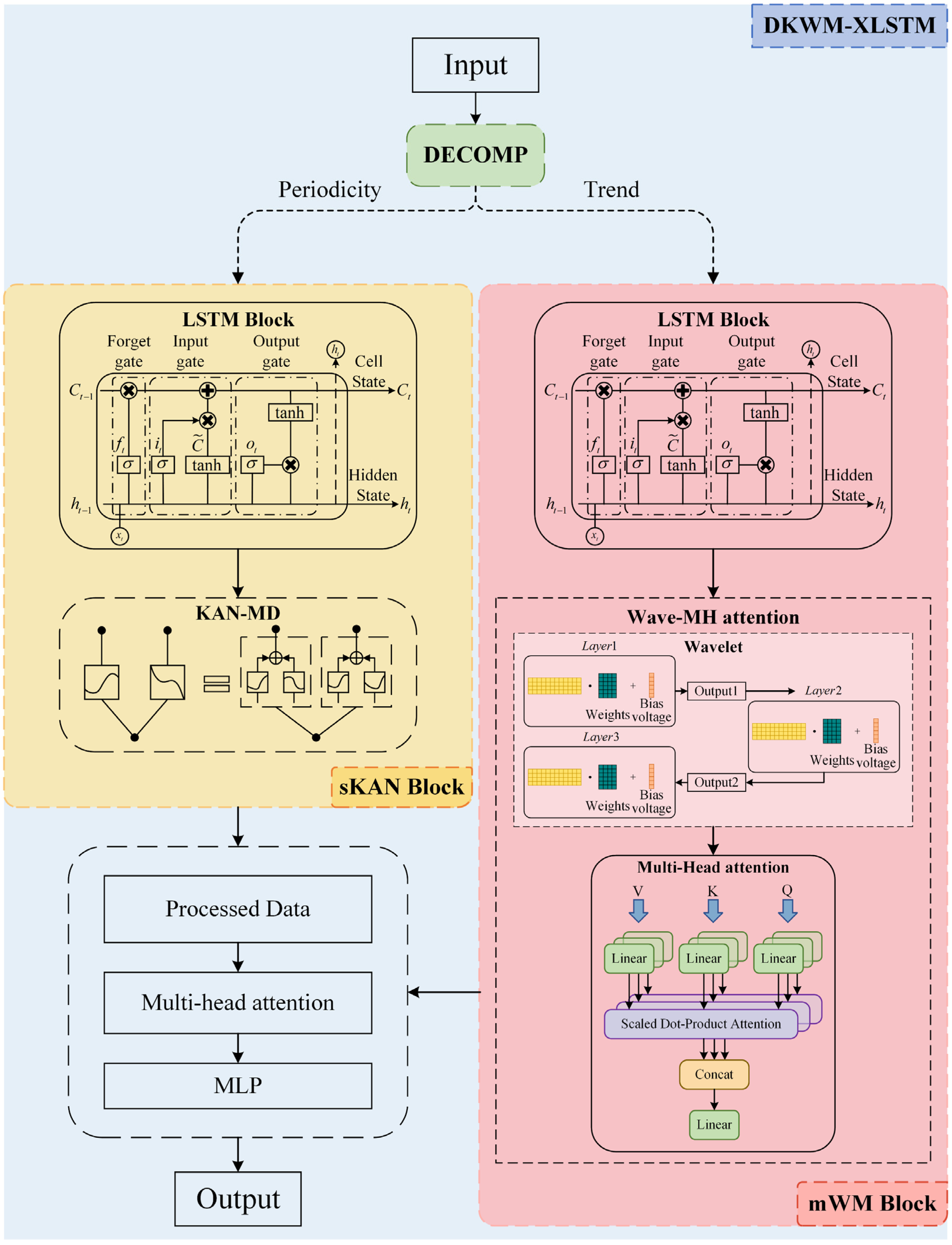
- We introduce a novel DKWM-XLSTM model (Enhancing XLSTM with Decomposition, KAN-MD, and Wave-MH Attention Mechanisms), which incorporates three innovative features designed to improve the model’s performance and stability.
- (a)
- We propose a novel Decomposition (DECOMP) module designed to decompose input time series data into two components: cyclical and trend. The cyclical component captures short-term fluctuations, while the trend component reveals long-term changes. Within the XLSTM network, the sLSTM Block focuses on the cyclical component, while the mLSTM Block addresses the trend component. This decomposition method enhances the robustness of time series forecasting and is integrated with module-specific processing in the carbon price forecasting model. This approach effectively mitigates the influence of multiple factors.
- (b)
- We propose a novel Kolmogorov–Arnold Network with Multi-Domain Diffusion (KAN-MD) module, which integrates with the sLSTM Block to form the new sKAN module. Its adaptive univariate function retains only the nonlinear dependencies between key factors, while suppressing the ineffective coupling of secondary factors, thereby dynamically eliminating redundant information. Furthermore, adjusting function parameters in an interpretable manner directly identifies the core driving factors, significantly enhancing the accuracy of feature extraction in the carbon price prediction model.
- (c)
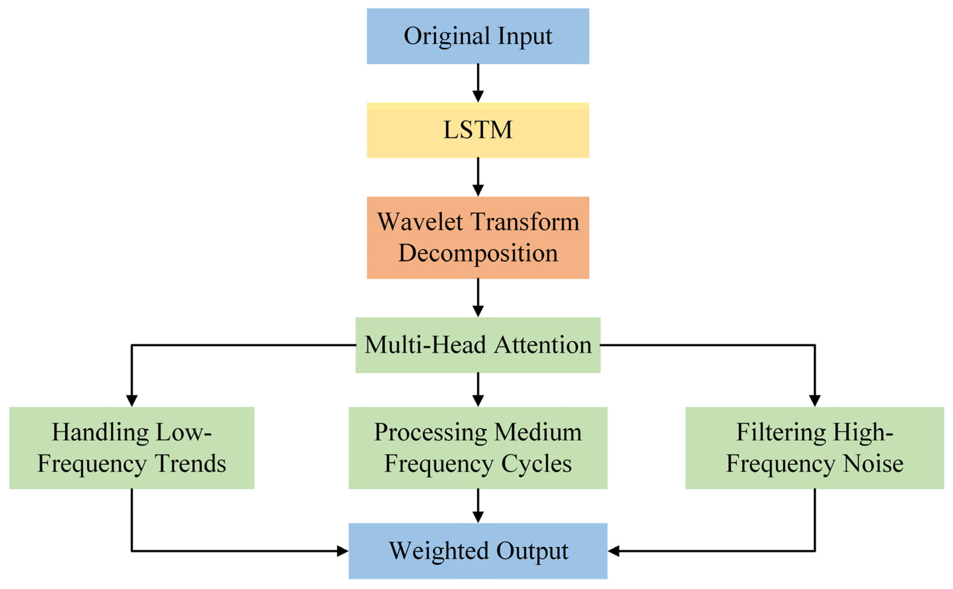
- We propose a novel Wave-Multi-Head Attention (Wave-MH attention) module, which integrates with the mLSTM Block to form the mWM module. The wavelet transform decomposes time series data into various frequency components, while the integration with the Multi-Head attention mechanism enables the model to focus on multiple dimensions of the input data and learn the relationships between different features. This combination allows the attention mechanism to concentrate on multi-scale features, thereby improving the model’s ability to mitigate the risks of overfitting and underfitting in carbon price prediction.
2. Materials and Methods
2.1. Data Acquisition and Processing
2.2. Method
2.2.1. Decomposition (DECOMP)
2.2.2. Kolmogorov–Arnold Networks with Multi-Domain Diffusion (KAN-MD)
2.2.3. Wave-Multi-Head Attention (Wave-MH Attention)
3. Result and Analysis
3.1. Experimental Environment and Training Details
3.2. Evaluation Indicators
- (1)
- Absolute error metrics include:
- (2)
- Relative error metrics include:
- (3)
- Goodness-of-fit metrics:
3.3. Ablation Experiments
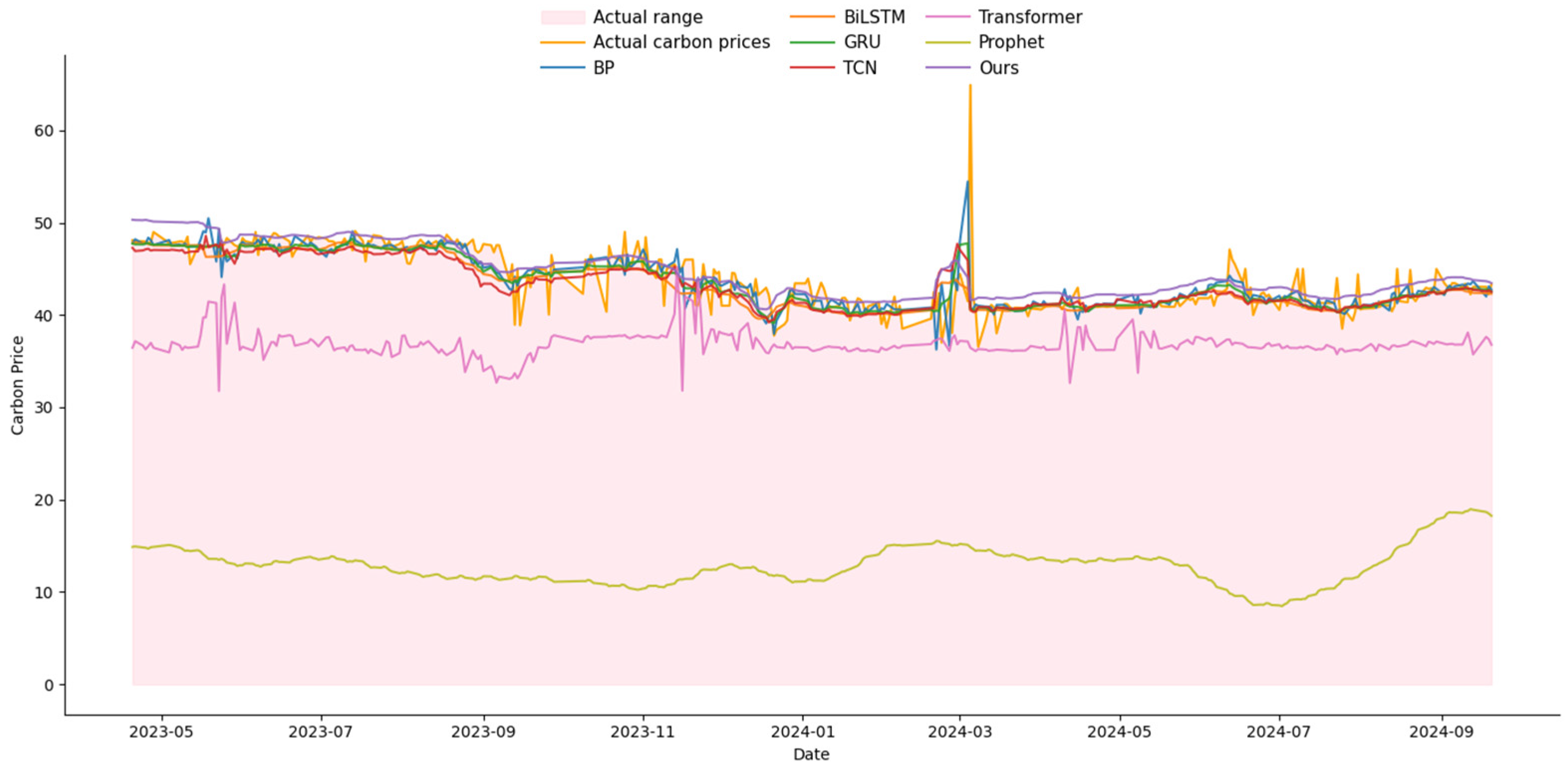
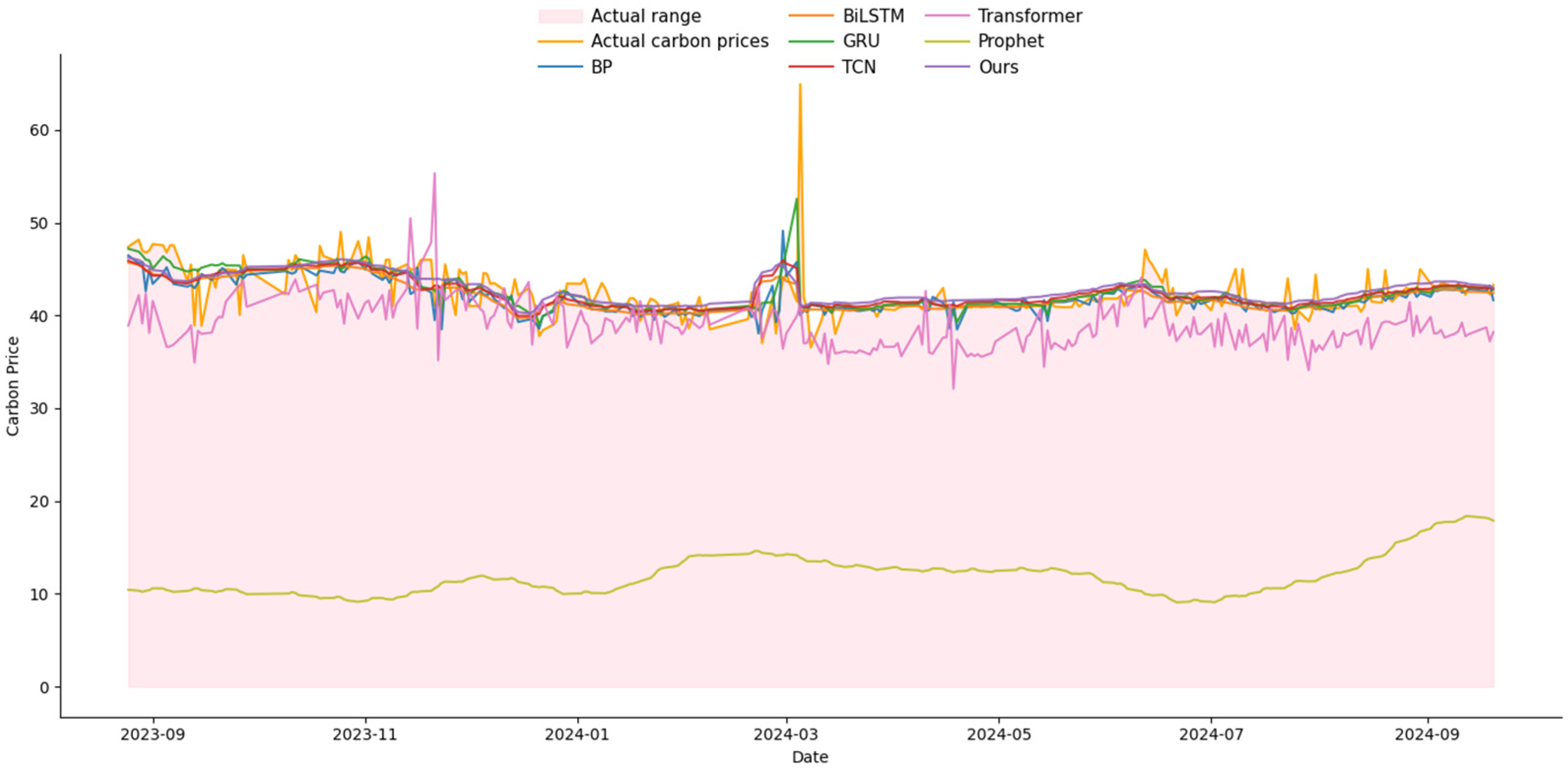
3.4. Comparison Experiments with Other Networks
3.5. Hyperparameter Optimization Experiments
4. Discussion
5. Conclusions
Author Contributions
Funding
Institutional Review Board Statement
Data Availability Statement
Conflicts of Interest
Abbreviations and Nomenclature
| Abbreviation | Definition |
| DECOMP | Decomposition |
| KAN-MD | Kolmogorov–Arnold Networks With Multi-Domain Diffusion |
| Wave-MH Attention | Wave-Multi-Head Attention |
| DKWM-XLSTM | Enhancing XLSTM With Decomposition, Kan-MD, And Wave-MH Attention Mechanisms |
| LSTM-CNN | Long Short-Term Memory and Convolutional Neural Network |
| GANs | Generative Adversarial Networks |
| ARIMA | Autoregressive Integrated Moving Average |
| ET-MVMD-LSTM | Extreme Random Trees and Multivariate Variational Modal Decomposition to Enhance Long Short-Term Memory |
| MEPT | Multiple Ensemble Patch Transformation |
| ICEEMDAN | Improved Adaptive Noise-Complete Ensemble Empirical Mode Decomposition |
| CTCNs | Causal Time Convolutional Networks |
| MIDE | Multi-Scale Interval Value Decomposition |
| NAMEMD | Noise-Assisted Multivariate Empirical Mode Decomposition |
| IVAR | Interval Value Vector Autoregression |
| IEA | Interval Event Analysis |
| IMLP | Interval Multi-Layer Perceptron |
| CEEMDAN | Complete Ensemble Empirical Mode Decomposition With Adaptive Noise |
| VMD | Variational Mode Decomposition |
| XGBoost | Extreme Gradient Boosting |
| PACF | Partial Autocorrelation Function |
| XLSTM | Extended Long Short-Term Memory |
| ADF | Augmented Dickey–Fuller |
| MLPs | Multi-Layer Perceptrons |
| CWT | Continuous Wavelet Transform |
| DWT | Discrete Wavelet Transform |
| MSE | Mean Squared Error |
| MAE | Mean Absolute Error |
| MAPE | Mean Absolute Percentage Error |
| R2 | Coefficient Of Determination |
| BP | Backpropagation |
| TCN | Temporal Convolutional Network |
| GRU | Gated Recurrent Unit |
| Bi-LSTM | Bidirectional Long Short-Term Memory |
| Transformer | Transformer Architecture |
| Propht | Prophet Forecasting Model |
| Nomenclature | Definition |
| Variables | |
| Y | Carbon Price |
| X1 | Market price of liquefied natural gas |
| X2 | Gasoline Price |
| X3 | Diesel Price |
| X4 | Gross Domestic Product (GDP) |
| X5 | Manufacturing Purchasing Managers’ Index (PMI) |
| X6 | Producer Price Index (PPI) |
| X7 | Consumer Price Index (CPI) |
| X8 | Inflation Rate |
| Parameters | |
| Total term of dataset | |
| Trend term of dataset | |
| Cyclical term of dataset | |
| m | The dynamic half-window width |
| P | The dominant cycle length |
| k | The neighborhood offset relative to the current calculation point t |
| Forgetting gate of the mWM block | |
| Input gate of the mWM block | |
| Output gate of the mWM block | |
| Cell state of the mWM block | |
| Hidden state of the mWM block | |
| The forgetting gate of the sKAN block | |
| The input gate of the sKAN block | |
| The output gate of the sKAN block | |
| The cell state of the sKAN block | |
| The hidden state of the sKAN block | |
| Combine the mWM block and sKAN block hidden states to generate the prediction results | |
| The final prediction result | |
| The weights of the fully connected layer | |
| The biases of the fully connected layer | |
| The weights of KAN-MD | |
| The biases of KAN-MD | |
| c | The number of layers of KAN-MD |
| The layer of KAN-MD | |
| The activation function of KAN-MD | |
| N | The number of samples |
| The true value of the i-th sample | |
| The predicted value of the i-th sample | |
| The parameters of KAN-MD | |
| The model parameter at the t-th iteration | |
| The learning rate of loss function | |
| The gradient of the loss function with respect to the parameter | |
| The input signal of wavelet transform | |
| The wavelet basis function | |
| a | The scale parameter of wavelet transform |
| b | The shift parameter of wavelet transform |
| The scale function of Haar wavelet | |
| Low-pass filter of scale function | |
| The wavelet function of Haar wavelet | |
| High-pass filter of wavelet function | |
| The approximation coefficient | |
| The detail coefficient | |
| Translation parameter | |
| Number of scales | |
| Q | Query matrix |
| K | Key matrix |
| V | Value matrix |
| T | The time step length of the input sequence |
| Query weight matrix | |
| Key weight matrix | |
| Value weight matrix | |
| The linear transformation matrix of the output | |
| The projection matrix of each attention head |
References
- Zhang, T.; Deng, M. A study on the differentiation of carbon prices in China: Insights from eight carbon emissions trading pilots. J. Clean. Prod. 2025, 501, 145279. [Google Scholar] [CrossRef]
- Song, Y.; Liu, T.; Ye, B.; Zhu, Y.; Li, Y.; Song, X. Improving the liquidity of China’s carbon market: Insights from the effect of carbon price transmission under policy release. J. Clean. Prod. 2019, 239, 118049. [Google Scholar] [CrossRef]
- Wang, S.; Wang, X.; Chen, S. Global value chains and carbon emission reduction in developing countries: Does industrial upgrading matter? Environ. Impact Assess. Rev. 2022, 97, 106895. [Google Scholar] [CrossRef]
- Zhu, H.; Goh, H.H.; Zhang, D.; Ahmad, T.; Liu, H.; Wang, S.; Wu, T. Key technologies for smart energy systems: Recent developments, challenges, and research opportunities in the context of carbon neutrality. J. Clean. Prod. 2022, 331, 129809. [Google Scholar] [CrossRef]
- Wan, L.; Tao, Y.; Wang, J.; Zhu, W.; Tang, C.; Zhou, G. A multi-scale multi-head attention network for stock trend prediction considering textual factors. Appl. Soft Comput. 2025, 171, 112388. [Google Scholar] [CrossRef]
- Cao, Y.; Zha, D.; Wang, Q.; Wen, L. Probabilistic carbon price prediction with quantile temporal convolutional network considering uncertain factors. J. Environ. Manag. 2023, 342, 118137. [Google Scholar] [CrossRef]
- Tanveer, U.; Ishaq, S.; Hoang, T.G. Enhancing carbon trading mechanisms through innovative collaboration: Case studies from developing nations. J. Clean. Prod. 2024, 482, 144122. [Google Scholar] [CrossRef]
- Liu, J.; Wang, P.; Chen, H.; Zhu, J. A combination forecasting model based on hybrid interval multi-scale decomposition: Application to interval-valued carbon price forecasting. Expert Syst. Appl. 2022, 191, 116267. [Google Scholar] [CrossRef]
- Huang, Y.; He, Z. Carbon price forecasting with optimization prediction method based on unstructured combination. Sci. Total Environ. 2020, 725, 138350. [Google Scholar] [CrossRef]
- Qin, Q.; Huang, Z.; Zhou, Z.; Chen, Y.; Zhao, W. Hodrick–Prescott filter-based hybrid ARIMA–SLFNs model with residual decomposition scheme for carbon price forecasting. Appl. Soft Comput. 2022, 119, 108560. [Google Scholar] [CrossRef]
- Adekoya, O.B. Predicting carbon allowance prices with energy prices: A new approach. J. Clean. Prod. 2021, 282, 124519. [Google Scholar] [CrossRef]
- Liu, J.P.; Zhang, X.B.; Song, X.H. Regional carbon emission evolution mechanism and its prediction approach driven by carbon trading: A case study of Beijing. J. Clean. Prod. 2018, 172, 2793–2810. [Google Scholar] [CrossRef]
- Zhang, X.; Yang, K.; Lu, Q.; Wu, J.; Yu, L.; Lin, Y. Predicting carbon futures prices based on a new hybrid machine learning: Comparative study of carbon prices in different periods. J. Environ. Manag. 2023, 346, 118962. [Google Scholar] [CrossRef] [PubMed]
- Xi, X.; Zhao, J.; Yu, L.; Wang, C. Exploring the potentials of artificial intelligence towards carbon neutrality: Technological convergence forecasting through link prediction and community detection. Comput. Ind. Eng. 2024, 190, 110015. [Google Scholar] [CrossRef]
- Shi, H.; Wei, A.; Xu, X.; Zhu, Y.; Hu, H.; Tang, S. A CNN-LSTM based deep learning model with high accuracy and robustness for carbon price forecasting: A case of Shenzhen’s carbon market in China. J. Environ. Manag. 2024, 352, 120131. [Google Scholar] [CrossRef]
- Huang, Z.; Zhang, W. Forecasting carbon prices in China’s pilot carbon market: A multi-source information approach with conditional generative adversarial networks. J. Environ. Manag. 2024, 359, 120967. [Google Scholar] [CrossRef]
- Yin, H.; Yin, Y.; Li, H.; Zhu, J.; Xian, Z.; Tang, Y.; Meng, A. Carbon emissions trading price forecasting based on temporal-spatial multidimensional collaborative attention network and segment imbalance regression. Appl. Energy 2025, 377, 124357. [Google Scholar] [CrossRef]
- Lu, H.; Ma, X.; Huang, K.; Azimi, M. Carbon trading volume and price forecasting in China using multiple machine learning models. J. Clean. Prod. 2020, 249, 119386. [Google Scholar] [CrossRef]
- Kumar, N.; Kayal, P.; Maiti, M. A study on the carbon emission futures price prediction. J. Clean. Prod. 2024, 483, 144309. [Google Scholar] [CrossRef]
- Zhang, K.; Yang, X.; Wang, T.; Thé, J.; Tan, Z.; Yu, H. Multi-step carbon price forecasting using a hybrid model based on multivariate decomposition strategy and deep learning algorithms. J. Clean. Prod. 2023, 405, 136959. [Google Scholar] [CrossRef]
- Li, D.; Li, Y.; Wang, C.; Chen, M.; Wu, Q. Forecasting carbon prices based on real-time decomposition and causal temporal convolutional networks. Appl. Energy 2023, 331, 120452. [Google Scholar] [CrossRef]
- Yang, K.; Sun, Y.; Hong, Y.; Wang, S. Forecasting interval carbon price through a multi-scale interval-valued decomposition ensemble approach. Energy Econ. 2024, 139, 107952. [Google Scholar] [CrossRef]
- Zhang, X.; Wang, J. An enhanced decomposition integration model for deterministic and probabilistic carbon price prediction based on two-stage feature extraction and intelligent weight optimization. J. Clean. Prod. 2023, 415, 137791. [Google Scholar] [CrossRef]
- Wang, J.; Zhuang, Z.; Gao, D. An enhanced hybrid model based on multiple influencing factors and divide-conquer strategy for carbon price prediction. Omega 2023, 120, 102922. [Google Scholar] [CrossRef]
- Wang, Y.; Qin, L.; Wang, Q.; Chen, Y.; Yang, Q.; Xing, L.; Ba, S. A novel deep learning carbon price short-term prediction model with dual-stage attention mechanism. Appl. Energy 2023, 347, 121380. [Google Scholar] [CrossRef]
- Ren, Y.; Huang, Y.; Wang, Y.; Xia, L.; Wu, D. Forecasting carbon price in Hubei Province using a mixed neural model based on mutual information and multi-head self-attention. J. Clean. Prod. 2025, 494, 144960. [Google Scholar] [CrossRef]
- Gianfreda, A.; Maranzano, P.; Parisio, L.; Pelagatti, M. Testing for integration and cointegration when time series are observed with noise. Econ. Model. 2023, 125, 106352. [Google Scholar] [CrossRef]
- Shojaie, A.; Fox, E.B. Granger causality: A review and recent advances. Annu. Rev. Stat. Appl. 2022, 9, 289–319. [Google Scholar] [CrossRef]
- He, Y.; Xing, Y.; Zeng, X.; Ji, Y.; Hou, H.; Zhang, Y.; Zhu, Z. Factors influencing carbon emissions from China’s electricity industry: Analysis using the combination of LMDI and K-means clustering. Environ. Impact Assess. Rev. 2022, 93, 106724. [Google Scholar] [CrossRef]
- Berrisch, J.; Pappert, S.; Ziel, F.; Arsova, A. Modeling volatility and dependence of European carbon and energy prices. Financ. Res. Lett. 2023, 52, 103503. [Google Scholar] [CrossRef]
- Balogun, A.L.; Tella, A. Modeling and investigating the impacts of climatic variables on ozone concentration in Malaysia using correlation analysis with random forest, decision tree regression, linear regression, and support vector regression. Chemosphere 2022, 299, 134250. [Google Scholar] [CrossRef]
- Zhou, F.; Huang, Z.; Zhang, C. Carbon price forecasting based on CEEMDAN and LSTM. Appl. Energy 2022, 311, 118601. [Google Scholar] [CrossRef]
- Zheng, G.; Li, K.; Yue, X.; Zhang, Y. A multifactor hybrid model for carbon price interval prediction based on decomposition-integration framework. J. Environ. Manag. 2024, 363, 121273. [Google Scholar] [CrossRef]
- Beck, M.; Pöppel, K.; Spanring, M.; Auer, A.; Prudnikova, O.; Kopp, M.; Hochreiter, S. XLSTM: Extended long short-term memory. arXiv 2024, arXiv:2405.04517. [Google Scholar] [CrossRef]
- Wu, D.; Ma, X.; Olson, D.L. Financial distress prediction using integrated Z-score and multilayer perceptron neural networks. Decis. Support Syst. 2022, 159, 113814. [Google Scholar] [CrossRef] [PubMed]
- Liu, Z.; Wang, Y.; Vaidya, S.; Ruehle, F.; Halverson, J.; Soljačić, M.; Tegmark, M. KAN: Kolmogorov-Arnold networks. arXiv 2024, arXiv:2404.19756. [Google Scholar] [CrossRef] [PubMed]
- Wen, X.; Zhou, M. Evolution and role of optimizers in training deep learning models. IEEE/CAA J. Autom. Sin. 2024, 11, 2039–2042. [Google Scholar] [CrossRef]
- Manikanta, V.; Vema, V.K. Formulation of wavelet-based multi-scale multi-objective performance evaluation (WMMPE) metric for improved calibration of hydrological models. Water Resour. Res. 2022, 58, e2020WR029355. [Google Scholar] [CrossRef]
- Hu, M.; Wu, C.; Zhang, L. GlobalMind: Global multi-head interactive self-attention network for hyperspectral change detection. ISPRS J. Photogramm. Remote Sens. 2024, 211, 465–483. [Google Scholar] [CrossRef]
- Doroshenko, L.; Mastroeni, L.; Mazzoccoli, A. Wavelet and deep learning framework for predicting commodity prices under economic and financial uncertainty. Mathematics 2025, 13, 1346. [Google Scholar] [CrossRef]
- Li, J.; Liu, D. Carbon price forecasting based on secondary decomposition and feature screening. Energy 2023, 278, 127783. [Google Scholar] [CrossRef]
- Sun, W.; Huang, C. A carbon price prediction model based on a secondary decomposition algorithm and optimized back propagation neural network. J. Clean. Prod. 2020, 243, 118671. [Google Scholar] [CrossRef]
- Zhang, X.; Zong, Y.; Du, P.; Wang, S.; Wang, J. Framework for multivariate carbon price forecasting: A novel hybrid model. J. Environ. Manag. 2024, 369, 122275. [Google Scholar] [CrossRef] [PubMed]
- Nadirgil, O. Carbon price prediction using multiple hybrid machine learning models optimized by genetic algorithm. J. Environ. Manag. 2023, 342, 118061. [Google Scholar] [CrossRef] [PubMed]
- Ji, M.; Du, J.; Du, P.; Niu, T.; Wang, J. A novel probabilistic carbon price prediction model: Integrating the transformer framework with mixed-frequency modeling at different quartiles. Appl. Energy 2025, 391, 125951. [Google Scholar] [CrossRef]
- Ghosh, I.; Jana, R.K. Clean energy stock price forecasting and response to macroeconomic variables: A novel framework using Facebook’s Prophet, NeuralProphet and explainable AI. Technol. Forecast. Soc. Change 2024, 200, 123148. [Google Scholar] [CrossRef]

| Category | Code | Symbol | Explanation |
|---|---|---|---|
| Energy | Y | Carbon Price | Price per ton of CO2 equivalent in carbon markets |
| X1 | Market Price of Liquefied Natural Gas | Market price of liquefied natural gas | |
| X2 | Gasoline Price | Per-unit price of gasoline in markets | |
| X3 | Diesel Price | Per-unit price of diesel in markets | |
| Economy | X4 | Gross Domestic Product (GDP) | Total economic output of a country |
| X5 | Manufacturing Purchasing Managers’ Index (PMI) | Indicating sector expansion or contraction | |
| X6 | Producer Price Index (PPI) | Tracking output price changes in industries | |
| Society | X7 | Consumer Price Index (CPI) | Measuring price changes of consumer goods or services |
| X8 | Inflation Rate | Percentage increase in general price level |
| Code | N | MEAN | SD | MIN | MEDIAN | MAX |
|---|---|---|---|---|---|---|
| lnY | 1853 | 3.4361 | 0.4398 | 2.4423 | 3.4648 | 10.6712 |
| lnX1 | 1853 | 8.4617 | 0.2751 | 7.8633 | 8.4338 | 9.1160 |
| lnX2 | 1853 | 9.0822 | 0.1236 | 8.8298 | 9.0797 | 9.3312 |
| lnX3 | 1853 | 8.9602 | 0.1334 | 8.6844 | 8.9625 | 9.2292 |
| X4 | 1659 | 0.3098 | 0.8948 | −2.3026 | 0.5878 | 1.6864 |
| lnX5 | 1853 | 4.6208 | 0.0123 | 4.5971 | 4.6214 | 4.6578 |
| lnX6 | 1853 | 4.6240 | 0.0437 | 4.5497 | 4.6092 | 4.7318 |
| lnX7 | 1853 | 3.9162 | 0.0379 | 3.5752 | 3.9160 | 3.9627 |
| lnX8 | 1853 | 11.6529 | 0.7817 | 10.0894 | 11.8357 | 12.7861 |
| Code | lnY | lnX1 | lnX2 | lnX3 | X4 | lnX5 | lnX6 | lnX7 | lnX8 |
|---|---|---|---|---|---|---|---|---|---|
| lnY | 1.0000 | ||||||||
| lnX1 | 0.3820 *** | 1.0000 | |||||||
| lnX2 | 0.5400 *** | 0.6339 *** | 1.0000 | ||||||
| lnX3 | 0.6282 *** | 0.5808 *** | 0.9009 *** | 1.0000 | |||||
| X4 | −0.2652 *** | −0.0960 *** | −0.2414 *** | −0.2066 *** | 1.0000 | ||||
| lnX5 | −0.2360 *** | −0.1718 *** | −0.2271 *** | −0.1697 *** | 0.8802 *** | 1.0000 | |||
| lnX6 | −0.2717 *** | 0.2876 *** | 0.0536 ** | −0.0513 ** | 0.1645 *** | 0.1024 *** | 1.0000 | ||
| lnX7 | −0.3374 *** | −0.1541 *** | −0.2511 *** | −0.3364 *** | −0.1038 *** | −0.1891 *** | 0.1715 *** | 1.0000 | |
| lnX8 | 0.8167 *** | 0.3376 *** | 0.4914 *** | 0.5753 *** | −0.4570 *** | −0.4115 *** | −0.3942 *** | −0.2990 *** | 1.0000 |
| Code | ADF Value | 1% Critical Value | 5% Critical Value | 10% Critical Value | Conclusion |
|---|---|---|---|---|---|
| lnY | −2.099 | −3.430 | −2.860 | −2.570 | Non-Stationary |
| d.lnY | −74.126 | −3.430 | −2.860 | −2.570 | Stationary |
| lnX1 | −3.113 | −3.430 | −2.860 | −2.570 | Stationary |
| d.lnX1 | −43.002 | −3.430 | −2.860 | −2.570 | Stationary |
| lnX2 | −1.631 | −3.430 | −2.860 | −2.570 | Non-Stationary |
| d.lnX2 | −43.003 | −3.430 | −2.860 | −2.570 | Stationary |
| lnX3 | −2.059 | −3.430 | −2.860 | −2.570 | Non-Stationary |
| d.lnX3 | −43.010 | −3.430 | −2.860 | −2.570 | Stationary |
| X4 | −1.800 | −3.430 | −2.860 | −2.570 | Non-Stationary |
| d.X4 | −40.597 | −3.430 | −2.860 | −2.570 | Stationary |
| lnX5 | −1.992 | −3.430 | −2.860 | −2.570 | Non-Stationary |
| d.lnX5 | −43.005 | −3.430 | −2.860 | −2.570 | Stationary |
| lnX6 | −1.044 | −3.430 | −2.860 | −2.570 | Non-Stationary |
| d.lnX6 | −43.026 | −3.430 | −2.860 | −2.570 | Stationary |
| lnX7 | −7.076 | −3.430 | −2.860 | −2.570 | Stationary |
| d.lnX7 | −43.000 | −3.430 | −2.860 | −2.570 | Stationary |
| lnX8 | −1.484 | −3.430 | −2.860 | −2.570 | Non-Stationary |
| d.lnX8 | −43.128 | −3.430 | −2.860 | −2.570 | Stationary |
| Training Set Ratio | Indicator | Haar | Meyer | Daubechies |
|---|---|---|---|---|
| 80% | MSE | 0.231% | 0.240% | 0.240% |
| MAE | 0.032 | 0.032 | 0.032 | |
| MAPE | 10.14 | 10.71 | 11.82 | |
| R2 | 95.36% | 95.35% | 95.53% | |
| 85% | MSE | 0.279% | 0.250% | 0.250% |
| MAE | 0.031 | 0.033 | 0.032 | |
| MAPE | 10.17 | 11.37 | 10.78 | |
| R2 | 94.57% | 95.14% | 95.12% |
| Designation | Version | |
|---|---|---|
| Hardware | CPU | Intel Xeon Platinum 8474C |
| RAM | 80 GB | |
| GPU | NVIDIA GeForce RTX 4090D (24GB) | |
| Hard disk | System disk:30 GB Data disk:50 GB | |
| Software | OS | Windows 11 ×64 |
| CUDA | 11.1 | |
| CUDNN | 8.0.5 | |
| Python | 3.11.9 | |
| Pytorch | 1.8.1 | |
| Tensorflow | 2.18.0 |
| Training Set Ratio | Group | DECOMP | KAN-MD | WAVE -MH Attention | MSE | RMSE | MAE | R2 |
|---|---|---|---|---|---|---|---|---|
| 80% | ① | -- | -- | -- | 0.237% | 10.04 | 0.0280 | 93.49% |
| ② | √ | 0.196% | 9.34 | 0.0273 | 96.21% | |||
| ③ | √ | 0.194% | 9.37 | 0.0274 | 95.22% | |||
| ④ | √ | 0.198% | 9.42 | 0.0262 | 95.87% | |||
| ⑤ | √ | √ | 0.193% | 9.26 | 0.0269 | 96.20% | ||
| ⑥ | √ | √ | 0.188% | 9.21 | 0.0277 | 96.81% | ||
| ⑦ | √ | √ | 0.185% | 9.18 | 0.0266 | 95.47% | ||
| ⑧ | √ | √ | √ | 0.184% | 9.07 | 0.0244 | 96.06% | |
| 85% | ① | -- | -- | -- | 0.230% | 11.12 | 0.0289 | 92.53% |
| ② | √ | 0.213% | 9.41 | 0.0269 | 87.85% | |||
| ③ | √ | 0.224% | 9.62 | 0.0282 | 91.12% | |||
| ④ | √ | 0.219% | 9.47 | 0.0273 | 89.64% | |||
| ⑤ | √ | √ | 0.225% | 13.12 | 0.0304 | 95.61% | ||
| ⑥ | √ | √ | 0.208% | 12.80 | 0.0277 | 93.61% | ||
| ⑦ | √ | √ | 0.214% | 11.72 | 0.0340 | 94.46% | ||
| ⑧ | √ | √ | √ | 0.218% | 11.05 | 0.0290 | 95.75% |
| Training Set Ratio | Indicator | BP | TCN | Bi-LSTM | GRU | Transformer | Prophet | Ours |
|---|---|---|---|---|---|---|---|---|
| 80% | MSE | 0.213% | 0.208% | 0.211% | 0.214% | 1.34% | 5.48% | 0.204% |
| MAE | 0.0283 | 0.0279 | 0.0284 | 0.0271 | 0.095 | 0.202 | 0.0277 | |
| MAPE | 9.52 | 9.59 | 9.62 | 9.26 | 31.14 | 128.79 | 9.25 | |
| R2 | 95.28% | 95.27% | 94.93% | 93.05% | 74.01% | −6.04% | 96.06% | |
| 85% | MSE | 0.250% | 0.233% | 0.253% | 0.217% | 1.43% | 5.47% | 0.218% |
| MAE | 0.0301 | 0.0313 | 0.0304 | 0.0274 | 0.095 | 0.202 | 0.0290 | |
| MAPE | 8.96 | 10.11 | 9.26 | 8.96 | 39.77 | 134.52 | 11.05 | |
| R2 | 93.13% | 92.47% | 92.08% | 93.77% | 72.19% | −6.64% | 95.75% |
| Size | MSE | MAE | MAPE | R2 |
|---|---|---|---|---|
| One | 0.215% [0.190%, 0.432%] | 0.0287 [0.0229, 0.0413] | 9.03 [8.81, 13.83] | 95.83% [91.83%, 96.69%] |
| Two | 0.209% [0.207%, 0.513%] | 0.0288 [0.0223, 0.0485] | 12.03 [11.23, 19.58] | 96.11% [90.18%, 94.89%] |
| Size | MSE | MAE | MAPE | R2 |
|---|---|---|---|---|
| [8, 16] | 0.200% | 0.0288 | 12.03 | 96.11% |
| [16, 32] | 0.202% | 0.0287 | 11.04 | 96.09% |
| [32, 64] | 0.204% | 0.0275 | 10.16 | 96.05% |
| [64, 128] | 0.211% | 0.0279 | 9.32 | 95.92% |
Disclaimer/Publisher’s Note: The statements, opinions and data contained in all publications are solely those of the individual author(s) and contributor(s) and not of MDPI and/or the editor(s). MDPI and/or the editor(s) disclaim responsibility for any injury to people or property resulting from any ideas, methods, instructions or products referred to in the content. |
© 2025 by the authors. Licensee MDPI, Basel, Switzerland. This article is an open access article distributed under the terms and conditions of the Creative Commons Attribution (CC BY) license (https://creativecommons.org/licenses/by/4.0/).
Share and Cite
Yu, Y.; Song, X.; Zhou, G.; Liu, L.; Pan, M.; Zhao, T. DKWM-XLSTM: A Carbon Trading Price Prediction Model Considering Multiple Influencing Factors. Entropy 2025, 27, 817. https://doi.org/10.3390/e27080817
Yu Y, Song X, Zhou G, Liu L, Pan M, Zhao T. DKWM-XLSTM: A Carbon Trading Price Prediction Model Considering Multiple Influencing Factors. Entropy. 2025; 27(8):817. https://doi.org/10.3390/e27080817
Chicago/Turabian StyleYu, Yunlong, Xuan Song, Guoxiong Zhou, Lingxi Liu, Meixi Pan, and Tianrui Zhao. 2025. "DKWM-XLSTM: A Carbon Trading Price Prediction Model Considering Multiple Influencing Factors" Entropy 27, no. 8: 817. https://doi.org/10.3390/e27080817
APA StyleYu, Y., Song, X., Zhou, G., Liu, L., Pan, M., & Zhao, T. (2025). DKWM-XLSTM: A Carbon Trading Price Prediction Model Considering Multiple Influencing Factors. Entropy, 27(8), 817. https://doi.org/10.3390/e27080817