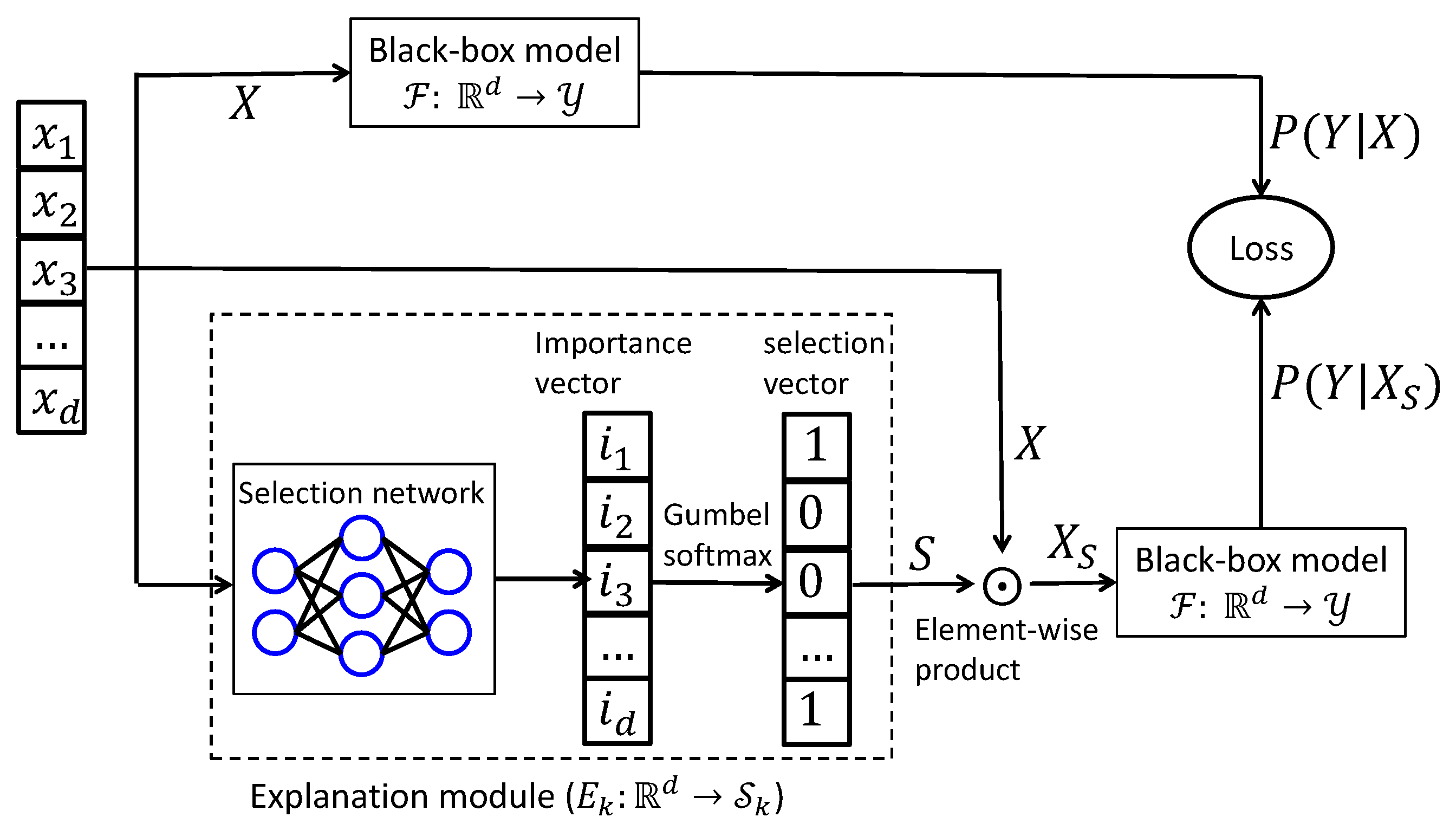
Figure 1.
Diagram of instance-wise causal feature selection. To generate explanations, each training sample is processed by an explainer network that produces a sparse binary mask of length d, indicating the top-k features selected for interpretation. This is achieved by first computing a causal influence score using the matrix-based Rényi’s -order entropy functional, followed by differentiable subset sampling using the Gumbel–Softmax trick to enable gradient-based optimization. The original input X and its masked counterpart are then passed through the black-box model to estimate their respective conditional outputs. These outputs are used to evaluate the objective function, and gradients are propagated back to update the parameters of the explainer network.
Figure 2.
Directed Acyclic Graph (DAG) describing our causal model. In our case, refers to the causal feature subset , whereas refers to the complement subset .
Figure 2.
Directed Acyclic Graph (DAG) describing our causal model. In our case, refers to the causal feature subset , whereas refers to the complement subset .
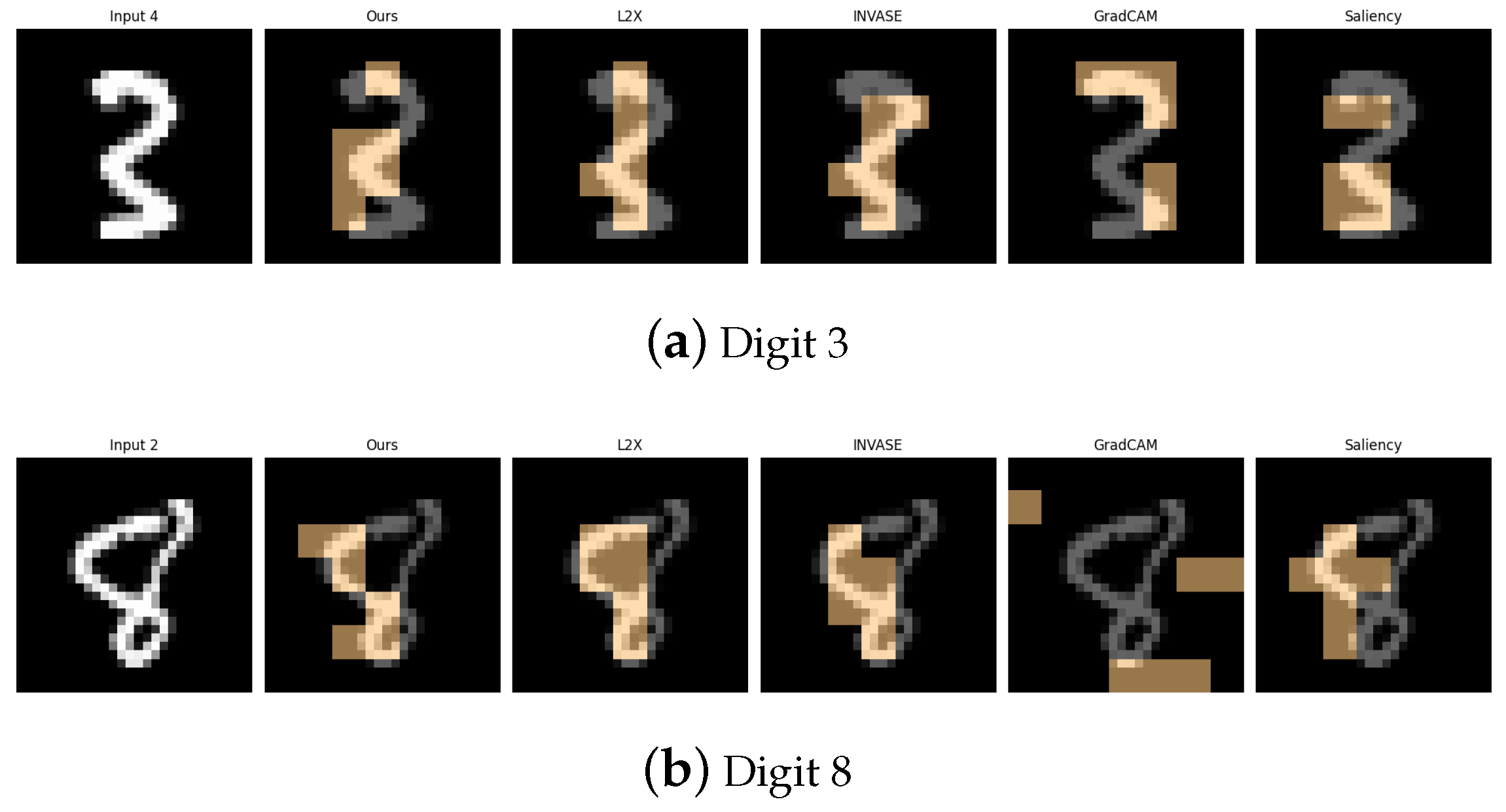
Figure 3.
Explanation visualizations of all competing methods on query images for the task of classifying digits 3 and 8. While both digits contain two stacked curves, the digit “8” forms a fully enclosed shape with connected loops, whereas “3” consists of two open arcs separated by a visible gap. Our method distinguishes between open and closed double-loop structures, offering improved interpretability.
Figure 4.
Explanation visualizations of all competing methods on query images for the task of classifying digits 1 and 7. Both digits are simple and share a similar top-down structure, but “1” is primarily a straight vertical line, whereas “7” includes an additional horizontal top stroke. Our method distinguishes between vertical and angular strokes, offering a more interpretable explanation of the model’s decision-making process.
Figure 5.
Explanation visualizations of all competing methods on query images for the task of classifying digits 0 and 6; “0” forms a perfect enclosed loop, whereas “6” introduces an additional tail or swirl at the bottom. Our method distinguishes between pure loops and loop-tail structures, effectively detecting such nuanced differences and offering more interpretable explanations.
Figure 6.
Explanation visualizations of all competing methods on query images for the task of classifying digits 2 and 5; “2” and “5” often appear visually similar in handwritten form, making them a challenging pair. Both digits contain multiple curves and sharp angles, requiring precise analysis of subtle geometric differences. Our method excels at the discrimination of fine-grained structures, leading to more interpretable and accurate explanations.
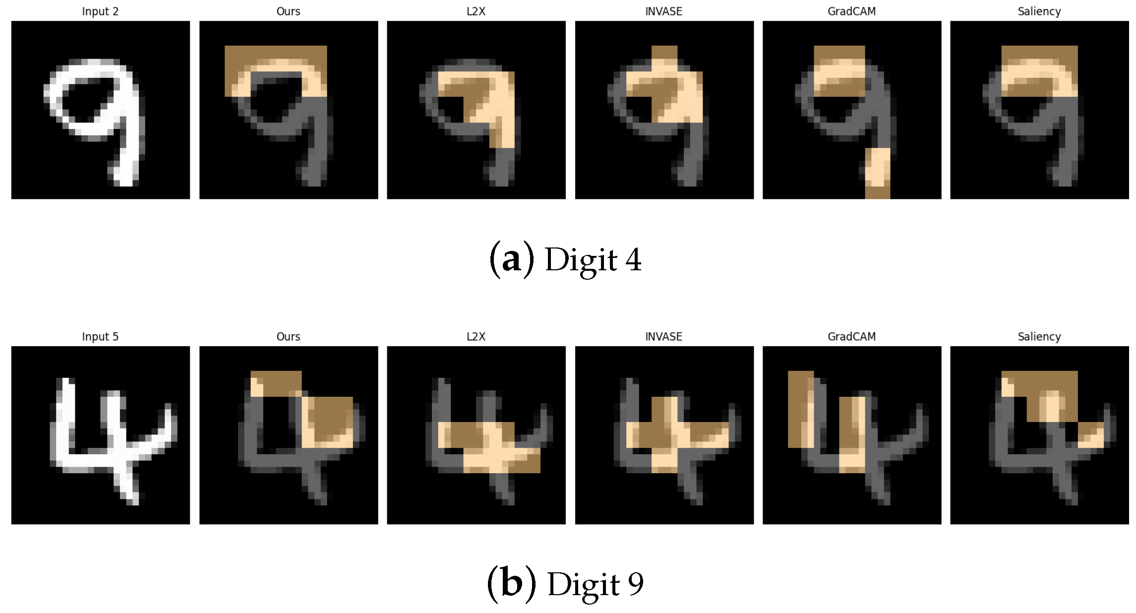
Figure 7.
Explanation visualizations of all competing methods on query images for the task of classifying digits 4 and 9; “4” is typically composed of straight lines, whereas “9” features a loop connected to a vertical stem. Our method effectively distinguishes between linear and curved structures, enabling the detection of both straight lines and enclosed loops for more interpretable decision-making.
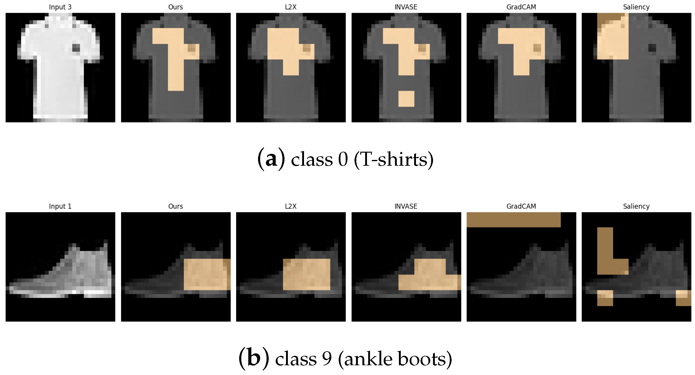
Figure 8.
Explanation visualizations of all competing methods on query images for the task of classifying class 0 (T-shirts) and class 9 (ankle boots). Our approach effectively distinguishes between upper-body and lower-body garments by capturing clear structural differences, such as soft fabric versus rigid materials.
Figure 9.
Explanation visualizations of all competing methods on query images for the task of classifying class 0 (T-shirts) and class 2 (pullovers). Class “0” (T-shirt) and class “2” (pullover) represent similar upper-body garments with subtle visual differences: T-shirts typically have shorter sleeves and a looser fit, whereas pullovers usually feature long sleeves and a more uniform texture. Our method effectively distinguishes between these characteristics, particularly sleeve length, resulting in higher accuracy and explanations that closely align with human perception.
Figure 10.
Explanation visualizations of all competing methods on query images for the task of classifying class 5 (sandals) and class 9 (ankle boots). Class “5” (sandal) and class “9” (ankle boot) represent two types of footwear with distinct visual characteristics—sandals are typically open-toed and lightweight, while ankle boots are enclosed and rigid. Our method effectively captures these structural differences, especially the presence or absence of open regions, leading to superior classification accuracy and interpretable attributions.
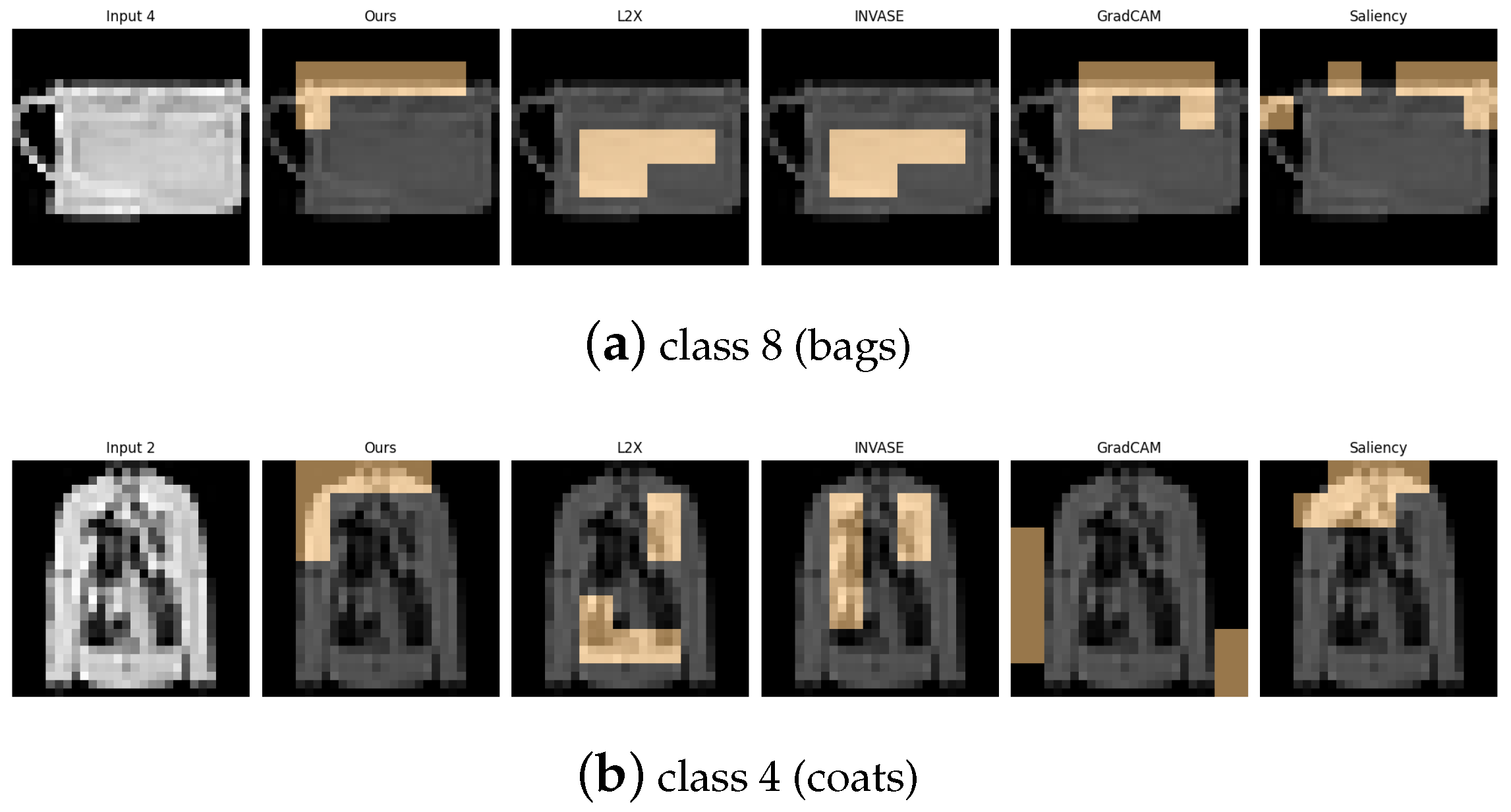
Figure 11.
Explanation visualizations of all competing methods on query images for the task of classifying class 8 (bags) and class 4 (coats). Class “8” (bag) and class “4” (coat) represent visually and functionally distinct categories—bags are typically compact and symmetric with handles, while coats are elongated garments with sleeves and complex contour lines. Our method captures these differences effectively, identifying key visual cues such as shoulder width and the presence of handles, resulting in accurate and interpretable predictions.
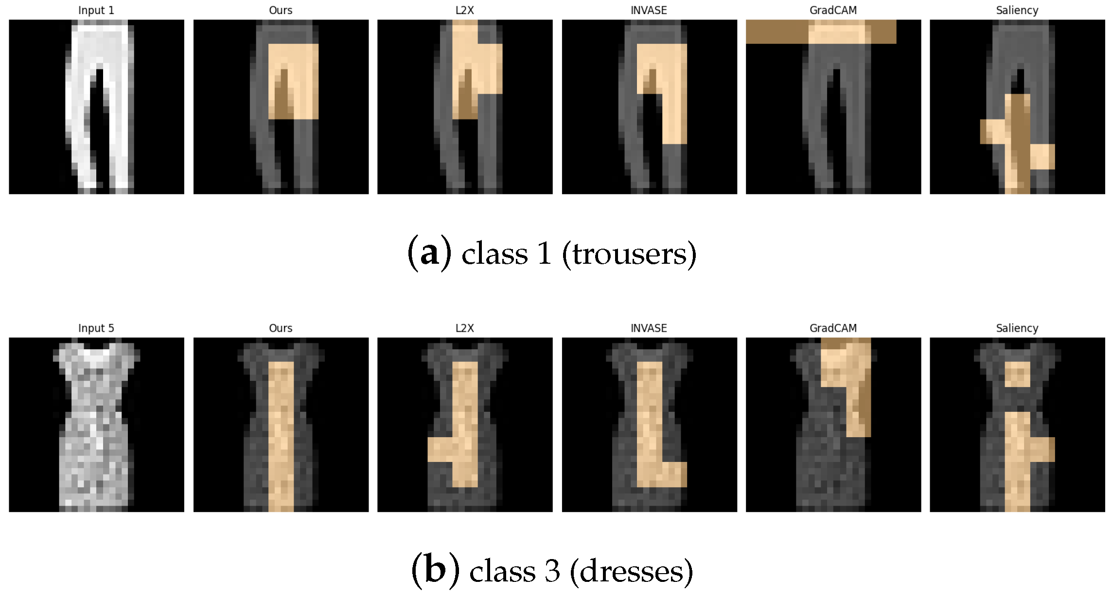
Figure 12.
Explanation visualizations of all competing methods on query images for the task of classifying class 1 (trousers) and class 3 (dresses). Our method demonstrates strong structural awareness when distinguishing between class “1” (trousers) and class “3” (dresses). For trousers, the explanation highlights the central hollow region between the two legs and the overall bilateral symmetry, key visual cues that align with human perception. In contrast, for dresses, which typically have a continuous lower contour, no such hollow region is detected. Instead, the explanation focuses on the single-piece flowing silhouette. These results illustrate the interpretability of our method in capturing meaningful structural differences between garment types.
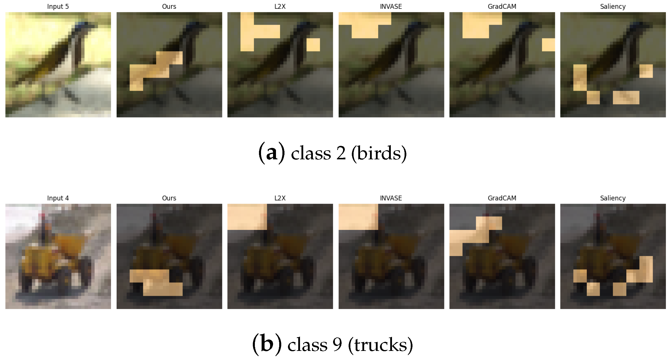
Figure 13.
Explanation visualizations of all competing methods on query images for the task of classifying class 2 (birds) and class 9 (trucks). Class “2” (birds) and class “9” (trucks) represent a high-level semantic contrast between natural and man-made objects. Birds are characterized by organic shapes, wings, and smooth contours, while trucks exhibit rigid structures with prominent components such as wheels and chassis. Our method accurately captures these key features by highlighting the wings and body contours of birds and the wheels and lower structure of trucks, resulting in both high classification accuracy and human-aligned interpretability.
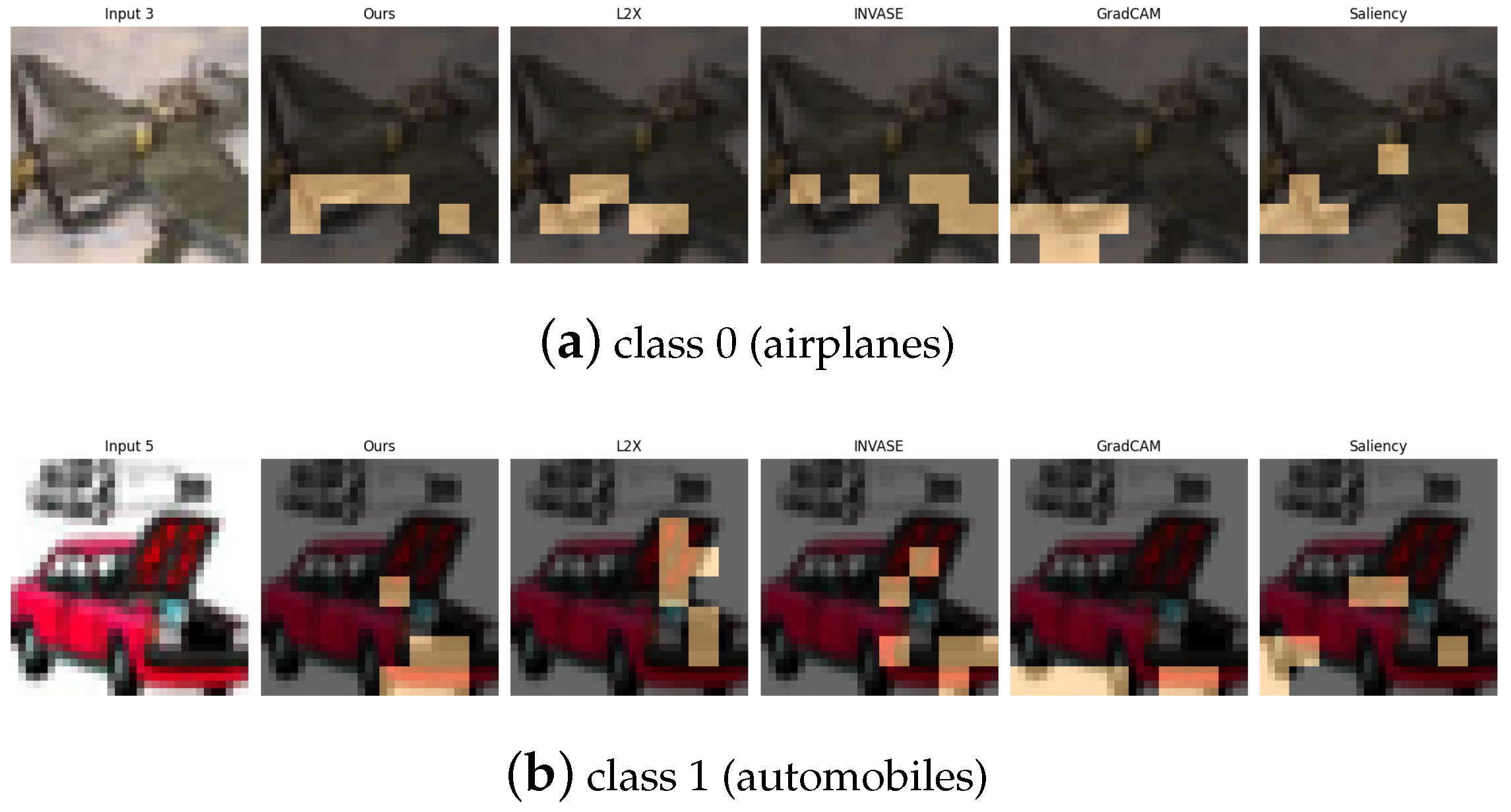
Figure 14.
Explanation visualizations of all competing methods on query images for the task of classifying class 0 (airplanes) and class 1 (automobiles). Class “0” (airplane) and class “1” (automobile) represent distinct categories of vehicles operating in different environments—air and ground. Airplanes are characterized by elongated fuselages, wings, and, in some cases, visible propellers, while automobiles are defined by compact bodies and wheels. Our method effectively captures these discriminative features, such as airplane wings and propellers and automobile wheels and chassis, resulting in high classification accuracy and semantically meaningful, human-aligned explanations.
Figure 15.
Explanation visualizations of all competing methods on query images for the task of classifying class 4 (deer) and class 7 (horses). Class “4” (deer) and class “7” (horse) both represent four-legged mammals with similar body plans, but differ in several fine-grained structural features. Our method demonstrates strong interpretability by highlighting class-specific anatomical and textural cues. For deer, it attends to the antlers, a distinctive feature not present in horses. For horses, it focuses on the solid-colored underbelly region. These explanations not only align well with human visual intuition but also reveal biologically meaningful cues that contribute to accurate and interpretable predictions.
Figure 16.
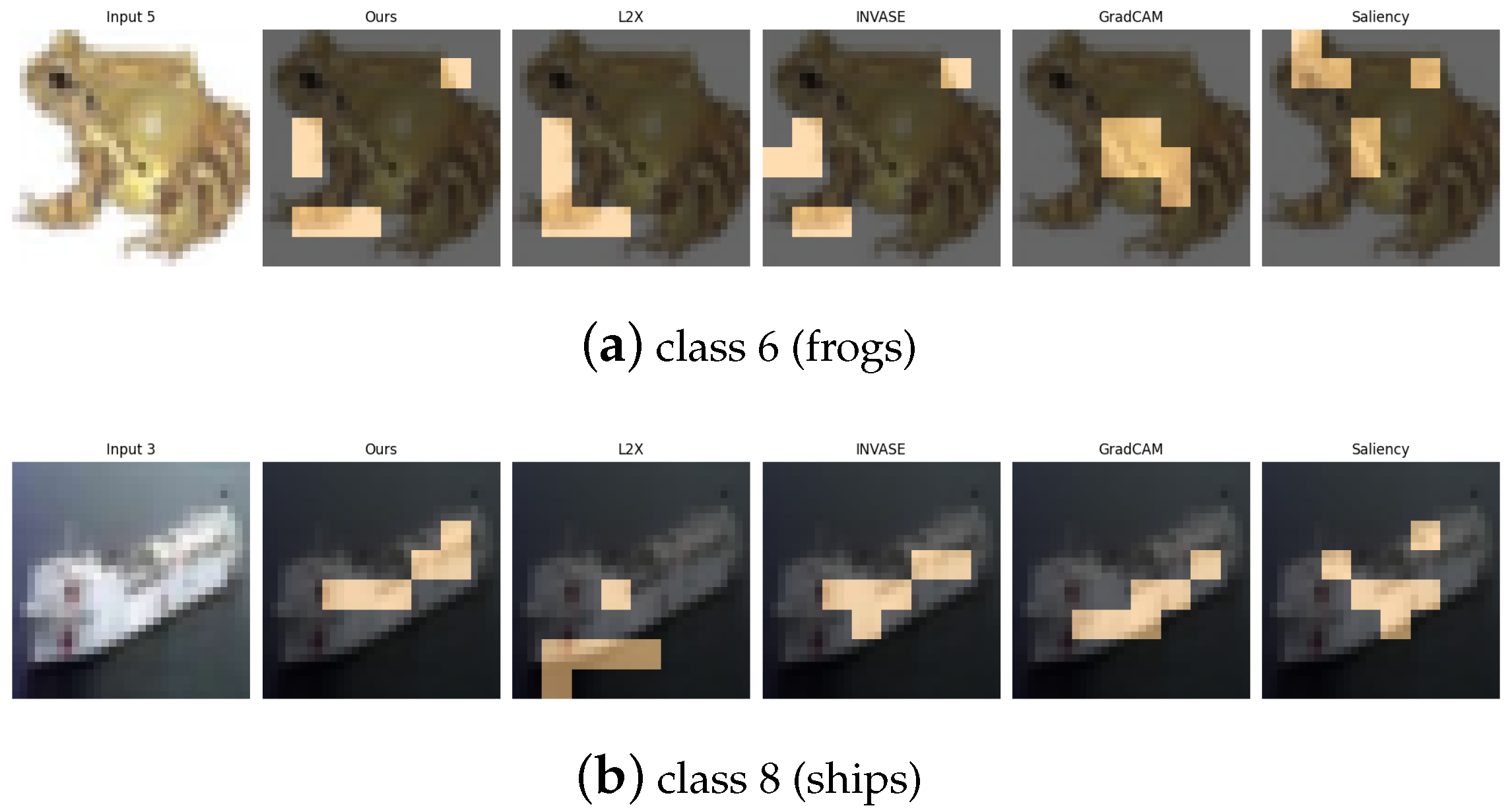
Explanation visualizations of all competing methods on query images for the task of classifying class 6 (frogs) and class 8 (ships). Class “6” (frog) and class “8” (ship) represent a contrast between natural and artificial objects. Frogs typically exhibit irregular, organic shapes, soft textures, and limb contours, while ships are rigid, geometrically structured, and often appear with horizontal decks. Our method captures these key differences effectively by focusing on features such as the leg outlines of frogs and the deck structures of ships, leading to improved performance and interpretable, semantically coherent explanations.
Figure 16.
Explanation visualizations of all competing methods on query images for the task of classifying class 6 (frogs) and class 8 (ships). Class “6” (frog) and class “8” (ship) represent a contrast between natural and artificial objects. Frogs typically exhibit irregular, organic shapes, soft textures, and limb contours, while ships are rigid, geometrically structured, and often appear with horizontal decks. Our method captures these key differences effectively by focusing on features such as the leg outlines of frogs and the deck structures of ships, leading to improved performance and interpretable, semantically coherent explanations.
Table 1.
Post-hoc accuracy (MNIST, 3 and 8). ** indicates statistically significant improvement over L2X at . The best performance is in bold.
Table 1.
Post-hoc accuracy (MNIST, 3 and 8). ** indicates statistically significant improvement over L2X at . The best performance is in bold.
| Method | k = 4 | k = 6 | k = 8 |
|---|
| Ours | ** | ** | ** |
| INVASE | | | |
| L2X | | | |
| GradCAM | | | |
| Saliency | | | |
Table 2.
Post-hoc accuracy (MNIST, 1 and 7). ** indicates statistically significant improvement over L2X at . The best performance is in bold.
Table 2.
Post-hoc accuracy (MNIST, 1 and 7). ** indicates statistically significant improvement over L2X at . The best performance is in bold.
| Method | k = 4 | k = 6 | k = 8 |
|---|
| Ours | ** | ** | ** |
| INVASE | | | |
| L2X | | | |
| GradCAM | | | |
| Saliency | | | |
Table 3.
Post-hoc accuracy (MNIST, 0 and 6). ** indicates statistically significant improvement over L2X at . The best performance is in bold.
Table 3.
Post-hoc accuracy (MNIST, 0 and 6). ** indicates statistically significant improvement over L2X at . The best performance is in bold.
| Method | k = 4 | k = 6 | k = 8 |
|---|
| Ours | ** | ** | ** |
| INVASE | | | |
| L2X | | | |
| GradCAM | | | |
| Saliency | | | |
Table 4.
Post-hoc accuracy (MNIST, 2 and 5). ** indicates statistically significant improvement over L2X at . The best performance is in bold.
Table 4.
Post-hoc accuracy (MNIST, 2 and 5). ** indicates statistically significant improvement over L2X at . The best performance is in bold.
| Method | k = 4 | k = 6 | k = 8 |
|---|
| Ours | ** | ** | ** |
| INVASE | | | |
| L2X | | | |
| GradCAM | | | |
| Saliency | | | |
Table 5.
Post-hoc accuracy (MNIST, 4 and 9). ** indicates statistically significant improvement over L2X at . The best performance is in bold.
Table 5.
Post-hoc accuracy (MNIST, 4 and 9). ** indicates statistically significant improvement over L2X at . The best performance is in bold.
| Method | k = 4 | k = 6 | k = 8 |
|---|
| Ours | ** | ** | ** |
| INVASE | | | |
| L2X | | | |
| GradCAM | | | |
| Saliency | | | |
Table 6.
Post-hoc accuracy (Fashion-MNIST, class 0 (T-shirts) and class 9 (ankle boots)). *, **, and *** indicate statistically significant improvement over L2X at , , and , respectively. The best performance is in bold.
Table 6.
Post-hoc accuracy (Fashion-MNIST, class 0 (T-shirts) and class 9 (ankle boots)). *, **, and *** indicate statistically significant improvement over L2X at , , and , respectively. The best performance is in bold.
| Method | k = 4 | k = 6 | k = 8 |
|---|
| Ours | *** | * | *** |
| INVASE | ** | | * |
| L2X | | | |
| GradCAM | | | |
| Saliency | | | |
Table 7.
Post-hoc accuracy (Fashion-MNIST, class 0 (T-shirts) and class 2 (pullovers)). *, **, and *** indicate statistically significant improvement over L2X at , , and , respectively. The best performance is in bold.
Table 7.
Post-hoc accuracy (Fashion-MNIST, class 0 (T-shirts) and class 2 (pullovers)). *, **, and *** indicate statistically significant improvement over L2X at , , and , respectively. The best performance is in bold.
| Method | k = 4 | k = 6 | k = 8 |
|---|
| Ours | *** | ** | *** |
| INVASE | ** | | * |
| L2X | | | |
| GradCAM | | | |
| Saliency | | | |
Table 8.
Post-hoc accuracy (Fashion-MNIST, class 5 (sandals) and class 9 (ankle boots)). *, **, and *** indicate statistically significant improvement over L2X at , , and , respectively. The best performance is in bold.
Table 8.
Post-hoc accuracy (Fashion-MNIST, class 5 (sandals) and class 9 (ankle boots)). *, **, and *** indicate statistically significant improvement over L2X at , , and , respectively. The best performance is in bold.
| Method | k = 4 | k = 6 | k = 8 |
|---|
| Ours | *** | ** | *** |
| INVASE | ** | | * |
| L2X | | | |
| GradCAM | | | |
| Saliency | | | |
Table 9.
Post-hoc accuracy (Fashion-MNIST, class 8 (bags) and class 4 (coats)). *, **, and *** indicate statistically significant improvement over L2X at , , and , respectively. The best performance is in bold.
Table 9.
Post-hoc accuracy (Fashion-MNIST, class 8 (bags) and class 4 (coats)). *, **, and *** indicate statistically significant improvement over L2X at , , and , respectively. The best performance is in bold.
| Method | k = 4 | k = 6 | k = 8 |
|---|
| Ours | *** | ** | *** |
| INVASE | ** | | * |
| L2X | | | |
| GradCAM | | | |
| Saliency | | | |
Table 10.
Post-hoc accuracy (Fashion-MNIST, class 1 (trousers) and class 3 (dresses)). *, **, and *** indicate statistically significant improvement over L2X at , , and , respectively. The best performance is in bold.
Table 10.
Post-hoc accuracy (Fashion-MNIST, class 1 (trousers) and class 3 (dresses)). *, **, and *** indicate statistically significant improvement over L2X at , , and , respectively. The best performance is in bold.
| Method | k = 4 | k = 6 | k = 8 |
|---|
| Ours | *** | ** | *** |
| INVASE | ** | | * |
| L2X | | | |
| GradCAM | | | |
| Saliency | | | |
Table 11.
Post-hoc accuracy (CIFAR-10, class 2 (birds) and class 9 (trucks)). *, **, and *** indicate statistically significant improvement over L2X at , , and , respectively. The best performance is in bold.
Table 11.
Post-hoc accuracy (CIFAR-10, class 2 (birds) and class 9 (trucks)). *, **, and *** indicate statistically significant improvement over L2X at , , and , respectively. The best performance is in bold.
| Method | 20% Pixels | 30% Pixels | 40% Pixels |
|---|
| Ours | ** | *** | *** |
| INVASE | * | ** | ** |
| L2X | | | |
| GradCAM | | | |
| Saliency | | | |
Table 12.
Post-hoc accuracy (CIFAR-10, class 0 (airplanes) and class 1 (automobiles)). *, **, and *** indicate statistically significant improvement over L2X at , , and , respectively. The best performance is in bold.
Table 12.
Post-hoc accuracy (CIFAR-10, class 0 (airplanes) and class 1 (automobiles)). *, **, and *** indicate statistically significant improvement over L2X at , , and , respectively. The best performance is in bold.
| Method | 20% Pixels | 30% Pixels | 40% Pixels |
|---|
| Ours | ** | *** | *** |
| INVASE | * | ** | ** |
| L2X | | | |
| GradCAM | | | |
| Saliency | | | |
Table 13.
Post-hoc accuracy (CIFAR-10, class 4 (deer) and class 7 (horses)). *, **, and *** indicate statistically significant improvement over L2X at , , and , respectively. The best performance is in bold.
Table 13.
Post-hoc accuracy (CIFAR-10, class 4 (deer) and class 7 (horses)). *, **, and *** indicate statistically significant improvement over L2X at , , and , respectively. The best performance is in bold.
| Method | 20% Pixels | 30% Pixels | 40% Pixels |
|---|
| Ours | ** | *** | *** |
| INVASE | * | ** | ** |
| L2X | | | |
| GradCAM | | | |
| Saliency | | | |
Table 14.
Post-hoc accuracy (CIFAR-10, class 6 (frogs) and class 8 (ships)). *, **, and *** indicate statistically significant improvement over L2X at , , and , respectively. The best performance is in bold.
Table 14.
Post-hoc accuracy (CIFAR-10, class 6 (frogs) and class 8 (ships)). *, **, and *** indicate statistically significant improvement over L2X at , , and , respectively. The best performance is in bold.
| Method | 20% Pixels | 30% Pixels | 40% Pixels |
|---|
| Ours | ** | *** | *** |
| INVASE | * | ** | ** |
| L2X | | | |
| GradCAM | | | |
| Saliency | | | |
Table 15.
Post-hoc accuracy (MNIST 3 vs. 8) for different values of in our method.
Table 15.
Post-hoc accuracy (MNIST 3 vs. 8) for different values of in our method.
| Method | k = 4 | k = 6 | k = 8 |
|---|
| Ours () | 0.947 ± 0.006 | 0.971 ± 0.006 | 0.981 ± 0.006 |
| Ours () | 0.951 ± 0.007 | 0.974 ± 0.004 | 0.984 ± 0.004 |
| Ours () | 0.948 ± 0.006 | 0.972 ± 0.006 | 0.982 ± 0.006 |
| Ours () | 0.945 ± 0.006 | 0.970 ± 0.006 | 0.978 ± 0.006 |
| Ours () | 0.942 ± 0.007 | 0.968 ± 0.007 | 0.975 ± 0.007 |
| Ours () | 0.939 ± 0.007 | 0.962 ± 0.007 | 0.972 ± 0.007 |
| Ours () | 0.936 ± 0.008 | 0.959 ± 0.008 | 0.969 ± 0.008 |
| Ours () | 0.934 ± 0.009 | 0.956 ± 0.009 | 0.967 ± 0.009 |
| Ours () | 0.931 ± 0.010 | 0.953 ± 0.010 | 0.964 ± 0.010 |
| Ours () | 0.929 ± 0.011 | 0.950 ± 0.011 | 0.962 ± 0.011 |
| INVASE | 0.945 ± 0.006 | 0.969 ± 0.005 | 0.982 ± 0.004 |


