Abstract
The ergodicity and ageing phenomena in a vibrational motor system driven by a periodic external force are investigated. Within the tailored parameter regime, the amplitude and frequency demonstrate contrasting effects on ergodicity. An increase of amplitude induces a transition from non-ergodic to ergodic behavior, whereas a higher driving frequency leads to a transition from ergodic to non-ergodic dynamics. These transitions are attributed to the enhanced ability of larger amplitudes to overcome potential energy barriers and the improved responsiveness of the system to external variations at lower frequencies. Moreover, pronounced ageing effects are observed at low amplitudes or high frequencies. These findings offer new insights into the intrinsic dynamical mechanisms of vibrational motor systems and provide a theoretical foundation for predicting their long-term operational performance.
1. Introduction
Ergodicity has always been a focal point of research in physics, chemistry, and biology, such as in quantum chaotic phenomena [1,2,3,4,5], continuous-time Markov processes [6], molecular collision and chemical reaction pathways [7,8,9], as well as molecular motion and diffusion in living cells [10,11]. According to Boltzmann–Gibbs statistics, if the observation time is much greater than the average waiting time, the system is ergodic [12]. However, conclusions drawn from single-molecule tracking experiments consistently contradict the assumption of ergodicity, and the phenomenon is referred to as ergodicity breaking [13,14]. The ergodicity breaking manifests in two different forms: (i) Strong ergodicity breaking, characterized by discontinuities in the state or phase space of the system, such as in the ageing of mean-field spin glasses [15] and quantum systems with local constraints [16]; (ii) Weak ergodicity breaking implies the existence of continuous regions, but the corresponding trajectories cannot completely sample them, even over an infinite period of time [17,18,19]. Experimentally, the ergodicity breaking has been observed in lipid particle diffusion within yeast cells [20], receptor motility in living cells [21], protein motility on human cell membranes [22], and single-particle tracking experiments [23]. Theoretically, the ergodicity breaking has been demonstrated in non-Hermitian many-body systems [24], constrained quantum systems [25], and Schwinger models [26].
The occurrence of ergodicity-breaking processes is typically accompanied by ageing [27,28,29]. Ageing refers to the dynamical process in which a system, remaining out of equilibrium over extended periods, exhibits observables (such as correlation and response functions) that explicitly depend on both the waiting time and observation time, thereby breaking time-translation invariance [27,30]. In disordered or glass systems, ageing manifests as slow relaxation dynamics, in which the ability of the system to explore its phase space is diminished, leading to an enhanced decomposition of ergodicity [31]. The link between ageing and ergodicity breaking has been demonstrated in physical systems ranging from spin glass to complex fluids, with ageing being the driving force behind the observed non-ergodic behavior [32,33].
Ergodicity is essential for understanding the behavior of a vibrational motor system over long time scales. As a periodic system operating under vibrational resonance conditions, the characteristic of the vibrational motor is that the traditional noise term is replaced by a time-periodic driving force with temporal symmetry [34,35,36]. In the prototype model of a vibrational motor [34], the introduction of additional driving terms can induce complex dynamic behaviors similar to randomness, which is a key aspect of understanding its dynamic response characteristics. By systematically modulating key parameters, the absolute negative mobility (ANM) phenomenon can be observed, with the system exhibiting a tendency to move in the direction opposite to the external force under vibrational driving [34]. At present, regarding the complex dynamical phenomena in the vibrational motor, existing studies have explored the control of anomalous transport by coexisting attractors [35], as well as anomalous diffusion and diffusion enhancement inside the vibrational motor [36]. However, although the dynamical phenomena in the vibrational motor have been extensively studied, research on the ergodicity and ageing characteristics of vibrational motors remains insufficient.
In this work, we investigate the ergodicity and ageing of a vibrational motor. We demonstrate that the emergence of non-ergodic behavior originates from two distinct mechanisms: at small amplitudes, the low-energy states of the system confine the particles within potential wells, whereas at high frequencies, the ability of the system to respond to external perturbations is limited, preventing adaptation to changes in external forces. Ageing is observed under both small amplitudes and high frequencies, indicating memory of the initial state and a waiting-time dependence of time-averaged observables. Additionally, we unveil the presence of anomalous diffusion in the system and elucidate the influence of external driving forces on the diffusion behavior.
The work is organized as follows: in Section 2 and Section 3 the model and observables are introduced, respectively. In Section 4 the theoretical analysis and numerical simulation of ergodicity properties are provided. Section 5 is dedicated to the discussion. And our conclusions are presented in Section 6.
2. Model
In the vibrational motor model, the dynamics of inertial particles moving in a spatially symmetric periodic potential under the influence of two time-periodic external forces is considered. The dimensionless equations of motion governing the particle dynamics are given as follows [34]:
where denotes the displacement of the inertial particle at time t, and is the friction coefficient. The dot and prime denote differentiation with respect to t and x, respectively. The external spatially symmetric periodic potential is with unit period. represents the first time-periodic signal with frequency and amplitude a. represents the second time-periodic signal with frequency and amplitude A. The constant bias force f is chosen to be negative, zero, or positive.
The first time-periodic signal is strong and can throw the system out of equilibrium. In contrast, the second time-periodic signal is weak and produces effects similar to noise. In the absence of the second signal, the system exhibits remarkably rich dynamical behavior in the asymptotic long time limit, including periodic motion, quasi-periodicity, and chaos [37,38,39]. Upon the introduction of a second signal, a series of anomalous transport phenomena can be observed, by tuning its driving amplitude and frequency, such as absolute negative mobility and diffusion enhancement [34,36]. The friction coefficient characterizes the damping effect arising from the interaction between the particle and its surrounding environment [40]. In the vibrational motor system, friction plays a crucial role in determining the dynamical response and energy dissipation properties. The coefficient governs the balance between the driving forces and dissipative effects, thereby influencing the ability of the system to sustain persistent motion and efficiently explore the phase space [29,35,36]. In the overdamped regime (large ), inertial effects vanish, and the particle motion becomes increasingly constrained, leading to enhanced localization [41]. In contrast, in the underdamped regime (small ), inertial effects become prominent, giving rise to richer dynamical behaviors, such as diffusion enhancement and complex transport phenomena [29,34,36].
3. Observables
The ensemble-averaged mean squared displacement () for a wide variety of systems often follows a power law scaling with time over broad time scales. The can be defined as
Deviations from normal Brownian motion () are a hallmark of anomalous diffusion, which encompasses subdiffusion () and superdiffusion () [13,17,42,43,44]. Specially, and −1 respectively correspond to ballistic diffusion and confined state [13,42,43,44]. Subdiffusion typically arises in complex media where particle motion is constrained, such as the cytoplasm or glassy materials [45,46]. Superdiffusion can be induced by persistent driving forces or long-range correlation mechanisms, such as in ordered driven systems or active matter [47,48].
To further investigate the ergodic properties of the system, the time-averaged mean squared displacement () is introduced, defined based on a single-particle trajectory as
where denotes the length of the time series and t denotes the lag time. The characterizes the spatial exploration capability of a particle along a single trajectory. If the distribution of over multiple particles is sufficiently concentrated, the and tend to coincide, indicating that the system is ergodic, i.e., time averages are equivalent to ensemble averages. In contrast, if from different trajectories still exhibit significant variability, the time- and ensemble-averaged mean squared displacement () is introduced to further characterize the system
The characterizes the overall average diffusive behavior of the system, reflecting its spatial sampling capability across multiple trajectories and time intervals.
To quantify the degree of fluctuations in the TMSD across different trajectories and to further assess the ergodic properties of the system, the ergodicity-breaking (EB) parameter is introduced
which provides an appropriate measure for describing the magnitude of fluctuations of . When , it indicates that the diffusive behavior among different particle trajectories is consistent, and the system satisfies ergodicity. In contrast, implies the presence of ergodicity breaking, meaning that even over an infinitely long observation time, a single trajectory is unable to fully explore the accessible phase space [23,49,50]. Therefore, the parameter not only quantifies the fluctuation of time-averaged observables among individual trajectories, but also serves to characterize the capability of the system to sample the phase space [13]. For a stationary process, the vanishing of the parameter is a sufficient condition for ergodicity.Therefore, before using , the stationarity of the process must be tested or the ensemble and time average must be compared (our system is stationary for a long time) [17,51]. The ratio of the time and ensemble-averaged can be employed.
Further, the amplitude scatter distribution of individual TMSD of trajectories is considered. The dimensionless parameter can be defined as
According to the Boltzmann–Khinchin ergodic hypothesis, the values and indicate, respectively, that the system does and does not satisfy ergodicity [17,52,53]. Additionally, physical observables, such as , may potentially depend on the time interval between the system’s initialization and the commencement of the measurement
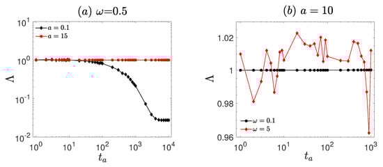
where is the ageing time. An ageing factor can be defined as
and indicates that there is no ageing in the system [54].
4. Results
The numerical simulations of Equation (1) are performed using the second-order Runge–Kutta method. The time step is set to , and the ensemble average is taken over trajectories, with uniformly distributed initial conditions. To investigate the ergodicity and ageing properties of the system, we consider the amplitude a and frequency of the first time-periodic signal as control parameters. First, we analyze the behavior of for various values of a and , as shown in Figure 1, discussing the diffusion characteristics of the system. In Figure 2, we present the representative particle trajectories under different parameter sets to provide intuitive insight into the dynamical behavior of the system. Subsequently, we examine and , illustrated in Figure 3, to explore the ergodicity of the system. The amplitude scattering function (, Figure 4) and ergodicity-breaking parameter (, Figure 5) are examined to further assess the ergodic properties of the system. Finally, the ageing behavior of the system and relevant ageing factors are analyzed (Figure 6 and Figure 7).
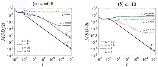
Figure 1.
The MSD/2t is governed by the dynamical Equation (1). (a) Different amplitudes a = 0.1, 7, 10, 15 with fixed frequency = 0.5. (b) Different frequencies = 0.1, 0.5, 1, 5 with fixed amplitude a = 10. The diffusion exponent is extracted by power-law fitting (black thin lines). The remaining parameters are set as , , , and . The diffusion behavior evolves with variations in amplitude and frequency, as indicated by the fitted black thin lines.
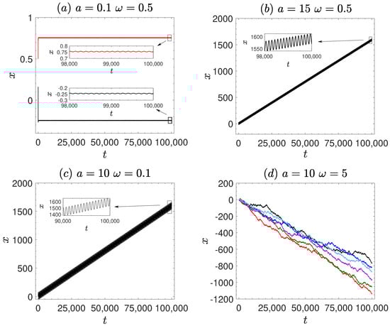
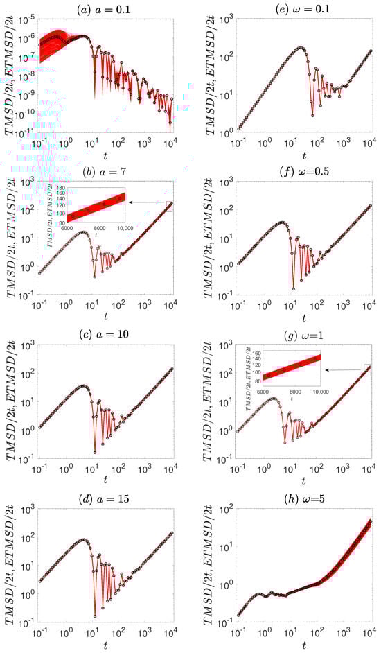
Figure 3.
The (marked by red solid lines) and (marked by black symbols) are governed by the dynamic Equation (1). The left column (a–d) corresponds to different external force amplitudes (a = 0.1, 7, 10, 15, respectively) with a fixed frequency . The right column (e–h) corresponds to different driving frequencies ( = 0.1, 0.5, 1, 5, respectively) with a fixed amplitude a = 10. The insets in panels (b,g) are enlarged to provide a more detailed view over specific time intervals. The remaining other parameters are the same as Figure 1.
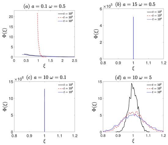
Figure 4.
The amplitude scattering distribution (, Equation (6)) corresponds to Figure 2. (a) The frequency = 0.5 and amplitude a = 0.1. (b) The frequency = 0.5 and amplitude a = 15. (c) The frequency = 0.1 and amplitude a = 10. (d) The frequency = 5 and amplitude a = 10. The remaining other parameters are the same as Figure 1.
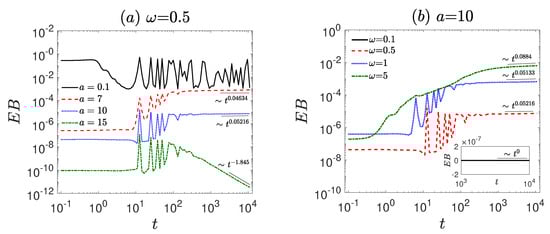
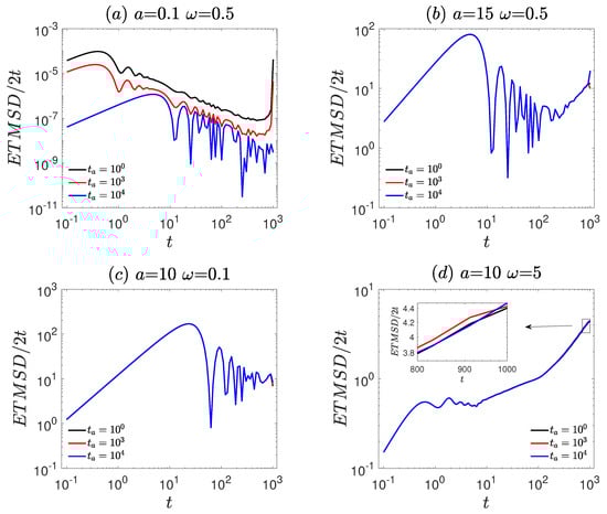
Figure 6.
The ageing characteristics of the vibrational motor are governed by the dynamic Equation (7). (a) The frequency = 0.5 and amplitude a = 0.1. (b) The frequency = 0.5 and amplitude a = 15. (c) The frequency = 0.1 and amplitude a = 10. (d) The frequency = 5 and amplitude a = 10. The remaining other parameters are the same as Figure 1.
Firstly, the anomalous diffusion behavior in the vibrational motor system is investigated (see Figure 1). For smaller amplitudes (, see Figure 1a), the system is confined ( −1). Under moderate external forces (e.g., and ), the system exhibits normal diffusion (). For relatively large amplitudes (e.g., ), the motion becomes confined again. As the amplitude increases, the system transitions from a confined state to normal diffusion, and at even higher amplitudes becomes confined again due to strong external driving.
Compared to amplitude, the influence of driving frequency on diffusion behavior exhibits a significantly different trend at lower driving frequencies. For a small driving frequency (, see Figure 1b), the system exhibits confined behavior characterized by −1. However, for moderate or large driving frequencies(, 1, and 5), the system displays normal diffusion (). As the amplitude of the external force increases, the diffusion changes from a confined state to normal diffusion.
To further understand the dynamical behavior of the particle, Figure 2 presents representative trajectories of a single particle under different parameter conditions. In Figure 2a, for a small amplitude a = 0.1, the particle remains confined near the symmetric periodic potential wells and only exhibits minor local oscillations. In contrast, Figure 2b corresponds to a large amplitude a = 15, where the driving force is significantly enhanced, allowing the particle to overcome the potential barriers and display a clear linear drift. In Figure 2c, under a low driving frequency = 0.1, the particle also exhibits pronounced directed motion, accompanied by strong periodic modulation. By comparison, Figure 2d shows the case of a higher frequency = 5, where the particle motion becomes more random and diffusive, and the trajectory overall displays a trend of gradual decay.
Meanwhile, in Figure 3, the relationship between and is considered. For smaller amplitudes, the is scattered around the in Figure 3a,b. This means that the system is non-ergodic. For larger amplitudes, the curves in Figure 3c,d are close to each other. This indicates that the system regains its ergodicity. Therefore, as the amplitude increases, the system changes from the ergodicity breaking to ergodicity. However, the effect of driving frequency on ergodicity is the opposite of the effect of amplitude on the ergodicity of the system. With the increase of driving frequency, the system changes from ergodicity to ergodicity-breaking (Figure 3e–h).
To elucidate the above non-ergodicity properties, the amplitude scattering distribution is employed to analyze the ergodicity of the system. At long time scales (especially at ), the distribution of is shown in Figure 4a–d. For a small amplitude ( and , Figure 4a), exhibits a broad, right-skewed profile, with the probability density primarily distributed at , indicating non-ergodicity. For a large amplitude ( and , Figure 4b), exhibits a pronounced peak at , i.e., ergodicity. For low frequency ( and , Figure 4c), a pronounced peak at is also observed, indicating ergodicity. In contrast, for high frequency ( and , Figure 4d), the distribution becomes substantially broader and more dispersed, with the probability density at markedly reduced compared to the ergodic cases, signifying ergodicity breaking. Overall, the amplitude scattering distribution further confirms the non-ergodic characteristics observed in Figure 3.
In addition, the ergodicity of the system is quantitatively analyzed through the ergodicity-breaking parameter (). For small amplitudes (see Figure 5a), the system is ergodicity-breaking (). As the amplitude increases, the value decreases (). This means that as the amplitude increases, the system changes from non-ergodicity to ergodicity. However, the amplitude and frequency demonstrate contrasting effects on ergodicity. As frequency increases, the system changes from ergodicity to non-ergodicity (Figure 5b).
The ageing characteristics of the system are presented in Figure 6. As observable from Figure 6, the behavior of exhibits a clear dependence on the ageing time . Specifically, Figure 6a,d shows clear trends, indicating significant ageing characteristics. However, in Figure 6b,c, the effect of ageing time on is relatively small, indicating that the ageing characteristics of the system are not significant. These observations demonstrate that the ageing effect is enhanced under small amplitudes or high driving frequencies.
The ageing behavior of the system is characterized by the ageing factor , as shown in Figure 7. At a fixed frequency (, Figure 7a), remains constant at unity () for large amplitude (). In contrast, for small amplitude (), decreases significantly as the ageing time increases and eventually stabilizes at , indicating pronounced ageing effects. At a fixed amplitude (, Figure 7b), is stable at unity () at low frequency (). For high frequency (), significant fluctuations of around unity are observed, indicating the presence of ageing.
5. Discussion
We investigate the influence of amplitude and frequency with respect to the ergodicity and ageing of a vibrational motor system. Regarding the ergodicity of the vibrational motor, an increase of amplitude induces a change from non-ergodic to ergodic behavior (Figure 3a–d). At smaller amplitudes, the system possesses lower energy and becomes localized within potential wells. This confinement hinders the ability of the system to effectively explore the entire phase space, leading to non-ergodic behavior. As observed in disordered systems, changes in energy states significantly impact ergodicity [27,28]. In our vibrational motor system, small amplitudes trap it within local energy regions. This energetic confinement leads to the emergence of non-ergodicity. Increasing the amplitude provides sufficient energy for the system to overcome potential barriers, enabling a more effective exploration of the entire phase space and thereby achieving ergodicity.
In contrast to the effect of amplitude, an increase in driving frequency drives the system from an ergodic to a non-ergodic state (Figure 3e–h). Higher driving frequencies prevent the system from responding promptly to changes in the external force, analogous to the Non-Poisson Recovery events observed in molecular diffusion [13,23]. In such systems, the memory of previous states is retained over long timescales, leading to a breakdown of ergodicity and a sluggish response to external perturbations. For instance, studies on non-Brownian diffusion in lipid membranes reveal that rapid changes in external conditions hinder the system from reaching a stable ergodic state [20]. Moreover, recent research by Liang et al. indicates that the non-ergodic characteristics of more general stochastic processes utilizing nonlinear clocks have been further examined, highlighting how spatiotemporal changes influence non-ergodicity [55]. In our vibrational motor system, the rapid variations induced by high-frequency external forces similarly impede the ability of the system to achieve ergodicity.
Concerning ageing characteristics, pronounced ageing effects are observed at small amplitudes and high frequencies (Figure 6a,d). This aligns with the ageing behavior in glassy systems, where systems exhibit non-stationary dynamics over long time scales [30,31]. At smaller amplitudes, ageing effects are more prominent. Due to the difficulty the system experiences in escaping local energy traps, its phase space exploration capability diminishes over time, leading to more pronounced ageing features. Conversely, at larger amplitudes and lower frequencies, the system more readily overcomes these traps, and ageing effects are relatively weaker.
As shown in Figure 7, the system exhibits pronounced ageing characteristics at small amplitudes and high frequencies. Specifically, for a small driving amplitude (, Figure 7a), decreases with ageing time and eventually stabilizes at . Under high-frequency driving (, Figure 7b), fluctuates around unity as the ageing time increases. These persistent deviations from indicate the presence of sustained ageing effects and ergodicity breaking in the system. This is consistent with weak ergodicity-breaking scenarios, where the time average does not converge to the ensemble average, even in the long-time limit [13,29]. Such behavior aligns with Bouchaud’s predictions for disordered systems, where ergodicity remains broken over extended periods due to the system being trapped in a hierarchy of metastable states, resulting in slow relaxation and persistent memory of initial conditions [27]. It is worthy of note that larger driving frequencies induce fluctuations in the ageing behavior (Figure 7b, ). As the frequency increases, the system undergoes more frequent temporal variations under the external force, placing it in a more dynamically evolving state.The ageing factor fluctuates around = 1. This is in agreement with findings reported in studies of the non-equilibrium dynamics of long—range spin—glass models [28,56], where the system response to time—varying external stimuli exhibits explicit time dependence. This time dependence leads to fluctuations in the ageing behavior, consistent with the phenomena observed in the vibrational motor system.
6. Conclusions
We report on the ergodicity breaking and ageing of a vibration motor system driven by periodic external forces. The results show that the emergence of non-ergodic behavior stems from two different mechanisms. The system remains localized within the potential well when the driving energy is insufficient at small amplitudes. Under high-frequency driving, the dynamic response is further suppressed because the driving period is shorter than the system’s intrinsic relaxation time. In contrast, increasing the driving amplitude provides sufficient energy for the system to overcome the potential barrier, while reducing the driving frequency allows the system to more effectively follow the external forcing. Furthermore, the ageing properties are most pronounced at low amplitudes and high frequencies, as evidenced by the explicit dependence of dynamical observables on the waiting time, reflecting the breakdown of time-translation invariance. These results reveal how the interaction between amplitude and frequency controls the ergodicity and ageing properties of vibrational motors, providing insights into the operational stability and long-term behavior of vibrational motors.
Author Contributions
Conceptualization, W.G. and L.D.; Software, W.G. and H.S.; Validation, Y.Y. and H.S.; Formal analysis, H.S.; Investigation, Y.Y. and L.D.; Resources, W.G.; Data curation, L.D.; Writing—original draft preparation, Y.Y.; Writing—review and editing, H.S. and W.G.; Visualization, Y.Y.; Supervision, W.G.; Project administration, W.G.; Funding acquisition, W.G. All authors have read and agreed to the published version of the manuscript.
Funding
This research was funded by the National Natural Science Foundation of China (Grant No. 12165010), the Yunnan Fundamental Research Project (Grants No. 202501AT070070 and 202401AT070422), the Xingdian Talent Support Project, the Young Top-notch Talent of Kunming and the Open Research Fund Program of the National Laboratory of Solid State Microstructures of Nanjing University (Grant No. M33020).
Institutional Review Board Statement
Not applicable.
Data Availability Statement
Data is contained within the article.
Conflicts of Interest
The authors declare no conflict of interest.
References
- Madhok, V.; Dogra, S.; Lakshminarayan, A. Quantum correlations as probes of chaos and ergodicity. Opt. Commun. 2018, 420, 189–193. [Google Scholar] [CrossRef]
- Piga, A.; Lewenstein, M.; Quach, J.Q. Quantum chaos and entanglement in ergodic and nonergodic systems. Phys. Rev. E 2019, 99, 032213. [Google Scholar] [CrossRef] [PubMed]
- Kos, P.; Bertini, B.; Prosen, T. Chaos and ergodicity in extended quantum systems with noisy driving. Phys. Rev. Lett. 2021, 126, 190601. [Google Scholar] [CrossRef] [PubMed]
- Serbyn, M.; Abanin, D.A.; Papić, Z. Quantum many-body scars and weak breaking of ergodicity. Nat. Phys. 2021, 17, 675–685. [Google Scholar] [CrossRef]
- Sinha, S.; Ray, S.; Sinha, S. Classical route to ergodicity and scarring in collective quantum systems. J. Phys. Condens. Matter 2024, 36, 163001. [Google Scholar] [CrossRef]
- Bellet, L.R. Ergodic properties of Markov processes. In Open Quantum Systems II: The Markovian Approach; Springer: Berlin/Heidelberg, Germany, 2006; pp. 1–39. [Google Scholar]
- Croft, J.F.; Bohn, J.L. Long-lived complexes and chaos in ultracold molecular collisions. Phys. Rev. A 2014, 89, 012714. [Google Scholar] [CrossRef]
- Dulieu, O.; Osterwalder, A. Cold Chemistry: Molecular Scattering and Reactivity Near Absolute Zero; Royal Society of Chemistry: Cambridge, UK, 2017. [Google Scholar]
- Liu, Y.; Luo, L. Molecular collisions: From near-cold to ultra-cold. Front. Phys. 2021, 16, 42300. [Google Scholar] [CrossRef]
- Klett, K.; Cherstvy, A.G.; Shin, J.; Sokolov, I.M.; Metzler, R. Non-Gaussian, transiently anomalous, and ergodic self-diffusion of flexible dumbbells in crowded two-dimensional environments: Coupled translational and rotational motions. Phys. Rev. E 2021, 104, 064603. [Google Scholar] [CrossRef]
- Barkai, E.; Garini, Y.; Metzler, R. Strange kinetics of single molecules in living cells. Phys. Today 2012, 65, 29–35. [Google Scholar] [CrossRef]
- Tsallis, C. Possible generalization of Boltzmann-Gibbs statistics. J. Stat. Phys. 1988, 52, 479–487. [Google Scholar] [CrossRef]
- Metzler, R.; Jeon, J.H.; Cherstvy, A.G.; Barkai, E. Anomalous diffusion models and their properties: Non-stationarity, non-ergodicity, and ageing at the centenary of single particle tracking. Phys. Chem. Chem. Phys. 2014, 16, 24128–24164. [Google Scholar] [CrossRef]
- Friedman, N.; Cai, L.; Xie, X.S. Stochasticity in Gene Expression as Observed by Single-molecule Experiments in Live Cells. Isr. J. Chem. 2009, 49, 333–342. [Google Scholar] [CrossRef]
- Bernaschi, M.; Billoire, A.; Maiorano, A.; Parisi, G.; Ricci-Tersenghi, F. Strong ergodicity breaking in aging of mean-field spin glasses. Proc. Natl. Acad. Sci. USA 2020, 117, 17522–17527. [Google Scholar] [CrossRef]
- Roy, S.; Lazarides, A. Strong ergodicity breaking due to local constraints in a quantum system. Phys. Rev. Res. 2020, 2, 023159. [Google Scholar] [CrossRef]
- Meroz, Y.; Sokolov, I.M. A toolbox for determining subdiffusive mechanisms. Phys. Rep. 2015, 573, 1–29. [Google Scholar] [CrossRef]
- Duan, Y.; Mahault, B.; Ma, Y.Q.; Shi, X.Q.; Chaté, H. Breakdown of ergodicity and self-averaging in polar flocks with quenched disorder. Phys. Rev. Lett. 2021, 126, 178001. [Google Scholar] [CrossRef]
- Shi, H.D.; Du, L.C.; Huang, F.J.; Guo, W. Collective topological active particles: Non-ergodic superdiffusion and ageing in complex environments. Chaos Solitons Fractals 2022, 157, 111935. [Google Scholar] [CrossRef]
- Metzler, R.; Jeon, J.H.; Cherstvy, A.G. Non-Brownian diffusion in lipid membranes: Experiments and simulations. Biochim. Biophys. Acta (BBA)-Biomembr. 2016, 1858, 2451–2467. [Google Scholar] [CrossRef] [PubMed]
- Manzo, C.; Torreno-Pina, J.A.; Massignan, P.; Lapeyre Jr, G.J.; Lewenstein, M.; Garcia Parajo, M.F. Weak ergodicity breaking of receptor motion in living cells stemming from random diffusivity. Phys. Rev. X 2015, 5, 011021. [Google Scholar] [CrossRef]
- Weigel, A.V.; Simon, B.; Tamkun, M.M.; Krapf, D. Ergodic and nonergodic processes coexist in the plasma membrane as observed by single-molecule tracking. Proc. Natl. Acad. Sci. USA 2011, 108, 6438–6443. [Google Scholar] [CrossRef] [PubMed]
- Burov, S.; Jeon, J.H.; Metzler, R.; Barkai, E. Single particle tracking in systems showing anomalous diffusion: The role of weak ergodicity breaking. Phys. Chem. Chem. Phys. 2011, 13, 1800–1812. [Google Scholar] [CrossRef]
- Chen, Q.; Chen, S.A.; Zhu, Z. Weak ergodicity breaking in non-Hermitian many-body systems. SciPost Phys. 2023, 15, 052. [Google Scholar] [CrossRef]
- Turner, C.J. Weak Ergodicity Breaking and Quantum Scars in Constrained Quantum Systems. Ph.D. Thesis, University of Leeds, Leeds, UK, 2019. [Google Scholar]
- Desaules, J.Y.; Banerjee, D.; Hudomal, A.; Papić, Z.; Sen, A.; Halimeh, J.C. Weak ergodicity breaking in the Schwinger model. Phys. Rev. B 2023, 107, L201105. [Google Scholar] [CrossRef]
- Bouchaud, J.P. Weak ergodicity breaking and aging in disordered systems. J. De Phys. I 1992, 2, 1705–1713. [Google Scholar] [CrossRef]
- Cugliandolo, L.F.; Kurchan, J. Analytical solution of the off-equilibrium dynamics of a long-range spin-glass model. Phys. Rev. Lett. 1993, 71, 173. [Google Scholar] [CrossRef] [PubMed]
- Guo, W.; Li, Y.; Song, W.-H.; Du, L.-C. Ergodicity breaking and ageing of underdamped Brownian dynamics with quenched disorder. J. Stat. Mech. Theory Exp. 2018, 2018, 033303. [Google Scholar] [CrossRef]
- Struik, L.C.E. Physical Aging in Amorphous Polymers and Other Materials; Elsevier Scientific Publishing Company: Amsterdam, The Netherlands, 1978; Volume 106. [Google Scholar]
- Horner, H. Glassy Dynamics and Aging in Disordered Systems. In Collective Dynamics of Nonlinear and Disordered Systems; Springer: Berlin/Heidelberg, Germany, 2005; pp. 203–236. [Google Scholar]
- Bouchaud, J.P.; Cugliandolo, L.F.; Kurchan, J.; Mezard, M. Out of equilibrium dynamics in spin-glasses and other glassy systems. Spin Glas. Random Fields 1998, 12, 161. [Google Scholar]
- Cipelletti, L.; Ramos, L. Slow dynamics in glassy soft matter. J. Phys. Condens Matter 2005, 17, R253. [Google Scholar] [CrossRef]
- Du, L.; Mei, D. Absolute negative mobility in a vibrational motor. Phys. Rev. E 2012, 85, 011148. [Google Scholar] [CrossRef]
- Du, L.; Mei, D. Coexisting attractors control of anomalous transport in a vibrational motor. Eur. Phys. J. B 2014, 87, 1–5. [Google Scholar] [CrossRef]
- Guo, W.; Du, L.C.; Mei, D.C. Anomalous diffusion and enhancement of diffusion in a vibrational motor. J. Stat. Mech. Theory Exp. 2014, 2014, P04025. [Google Scholar] [CrossRef]
- Kautz, R.L. Noise, chaos, and the Josephson voltage standard. Rep. Prog. Phys. 1996, 59, 935. [Google Scholar] [CrossRef]
- Jung, P.; Kissner, J.G.; Hänggi, P. Regular and chaotic transport in asymmetric periodic potentials: Inertia ratchets. Phys. Rev. Lett. 1996, 76, 3436. [Google Scholar] [CrossRef] [PubMed]
- Mateos, J.L. Chaotic transport and current reversal in deterministic ratchets. Phys. Rev. Lett. 2000, 84, 258. [Google Scholar] [CrossRef]
- Risken, H. Fokker-Planck Equation for One Variable; Methods of Solution. In The Fokker-Planck Equation: Methods of Solution and Applications; Springer: Berlin/Heidelberg, Germany, 1996; pp. 96–132. [Google Scholar]
- Fieguth, D.M. Dynamical active particles in the overdamped limit. J. Phys. Commun. 2024, 8, 075001. [Google Scholar] [CrossRef]
- Bouchaud, J. P; Georges, A. Anomalous diffusion in disordered media: Statistical mechanisms, models and physical applications. Phys. Rep. 1990, 195, 127–293. [Google Scholar] [CrossRef]
- Sancho, J.M.; Lacasta, A.; Lindenberg, K.; Sokolov, I.M.; Romero, A. Diffusion on a solid surface: Anomalous is normal. Phys. Rev. Lett. 2004, 92, 250601. [Google Scholar] [CrossRef]
- Khoury, M.; Lacasta, A.M.; Sancho, J.M.; Lindenberg, K. Weak Disorder: Anomalous Transport and Diffusion Are Normal Yet Again. Phys. Rev. Lett. 2011, 106, 090602. [Google Scholar] [CrossRef]
- Weiss, M.; Elsner, M.; Kartberg, F.; Nilsson, T. Anomalous subdiffusion is a measure for cytoplasmic crowding in living cells. Biophys. J. 2004, 87, 3518–3524. [Google Scholar] [CrossRef]
- Golding, I.; Cox, E.C. Physical nature of bacterial cytoplasm. Phys. Rev. Lett. 2006, 96, 098102. [Google Scholar] [CrossRef]
- Ramaswamy, S. The mechanics and statistics of active matter. Annu. Rev. Condens. Matter Phys 2010, 1, 323–345. [Google Scholar] [CrossRef]
- Bechinger, C.; Di Leonardo, R.; Löwen, H.; Reichhardt, C.; Volpe, G.; Volpe, G. Active particles in complex and crowded environments. Rev. Mod. Phys. 2016, 88, 045006. [Google Scholar] [CrossRef]
- Cherstvy, A.G.; Thapa, S.; Mardoukhi, Y.; Chechkin, A.V.; Metzler, R. Time averages and their statistical variation for the Ornstein-Uhlenbeck process: Role of initial particle distributions and relaxation to stationarity. Phys. Rev. E 2018, 98, 022134. [Google Scholar] [CrossRef] [PubMed]
- He, Y.; Burov, S.; Metzler, R.; Barkai, E. Random time-scale invariant diffusion and transport coefficients. Phys. Rev. Lett. 2008, 101, 058101. [Google Scholar] [CrossRef] [PubMed]
- Thiel, F.; Sokolov, I.M. Scaled Brownian motion as a mean-field model for continuous-time random walks. Phys. Rev. E 2014, 89, 012115. [Google Scholar] [CrossRef]
- Burov, S.; Metzler, R.; Barkai, E. Aging and nonergodicity beyond the Khinchin theorem. Proc. Natl. Acad. Sci. USA 2010, 107, 13228–13233. [Google Scholar] [CrossRef]
- Cherstvy, A.G.; Wang, W.; Metzler, R.; Sokolov, I.M. Inertia triggers nonergodicity of fractional Brownian motion. Phys. Rev. E 2021, 104, 024115. [Google Scholar] [CrossRef]
- Safdari, H.; Cherstvy, A.G.; Chechkin, A.V.; Thiel, F.; Sokolov, I.M.; Metzler, R. Theoretical. Quantifying the non-ergodicity of scaled Brownian motion. J. Phys. A: Math. Theor. 2015, 48, 375002. [Google Scholar] [CrossRef]
- Liang, Y.; Wang, W.; Metzler, R.; Cherstvy, A.G. Anomalous diffusion, nonergodicity, non-Gaussianity, and aging of fractional Brownian motion with nonlinear clocks. Phys. Rev. E 2023, 108, 034113. [Google Scholar] [CrossRef]
- Christiansen, H.; Majumder, S.; Henkel, M.; Janke, W. Aging in the long-range Ising model. Phys. Rev. Lett. 2020, 125, 180601. [Google Scholar] [CrossRef]
Disclaimer/Publisher’s Note: The statements, opinions and data contained in all publications are solely those of the individual author(s) and contributor(s) and not of MDPI and/or the editor(s). MDPI and/or the editor(s) disclaim responsibility for any injury to people or property resulting from any ideas, methods, instructions or products referred to in the content. |
© 2025 by the authors. Licensee MDPI, Basel, Switzerland. This article is an open access article distributed under the terms and conditions of the Creative Commons Attribution (CC BY) license (https://creativecommons.org/licenses/by/4.0/).