
Entropy Generation Optimization in Multidomain Systems: A Generalized Gouy-Stodola Theorem and Optimal Control


Abstract
1. Introduction
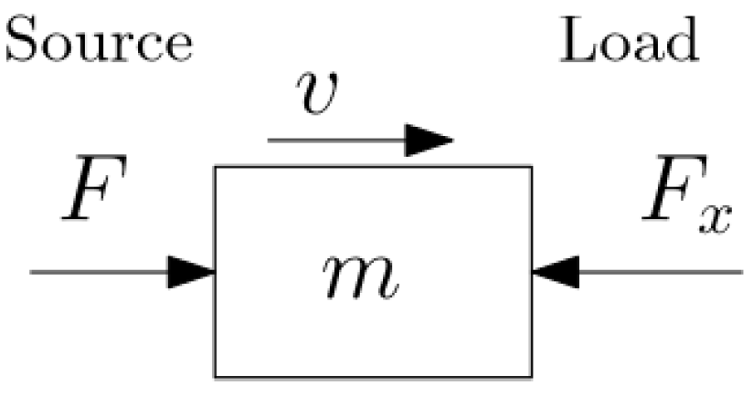
1.1. Instantaneous Energy Directionality
1.2. Extended Interpretations of the SLT and Cyclo-Dissipativity
1.3. Entropy Generation Minimization and the Gouy-Stodola Theorem
Entropy Generation
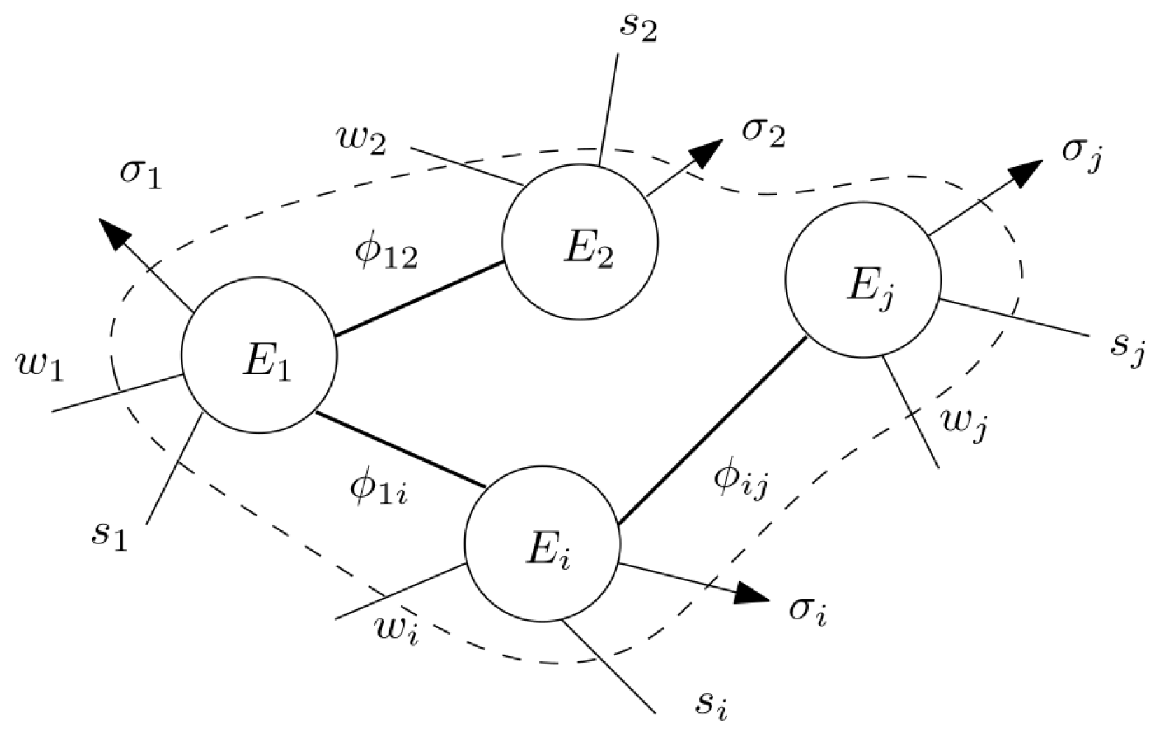
2. Interconnected System and Average Power Balances
Cyclic Trajectories
3. Generalized Thermodynamic Systems
3.1. Directionality Axiom
3.2. Thermodynamically-Consistent Work
3.3. Average Entropy Generation and Clausius Inequality
3.4. The Gouy-Stodola Theorem for Interconnected Systems
3.5. Other Forms of Work
4. Multidomain Systems
4.1. Energy Cyclo-Directionality Property (ECD)
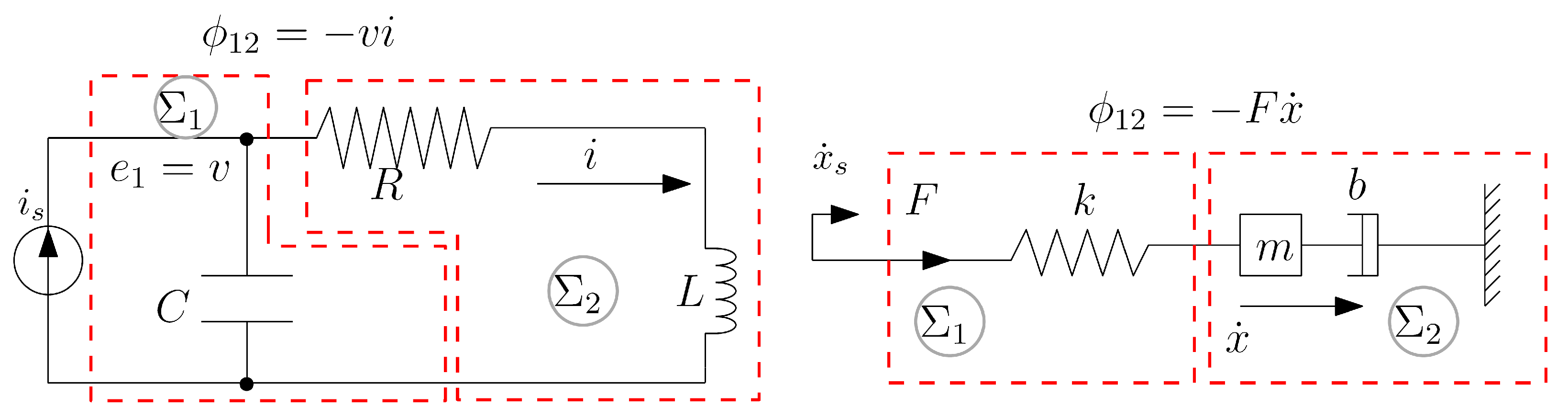
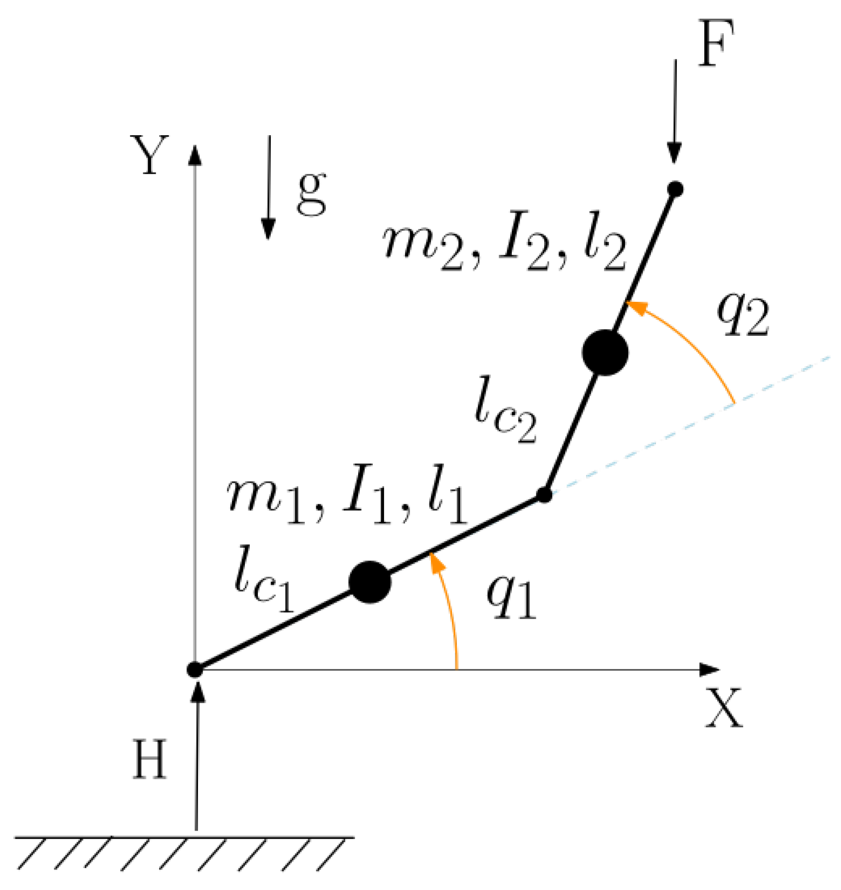
4.2. ECD for Three Example Systems
4.3. The Gouy-Stodola Theorem for Multidomain Systems
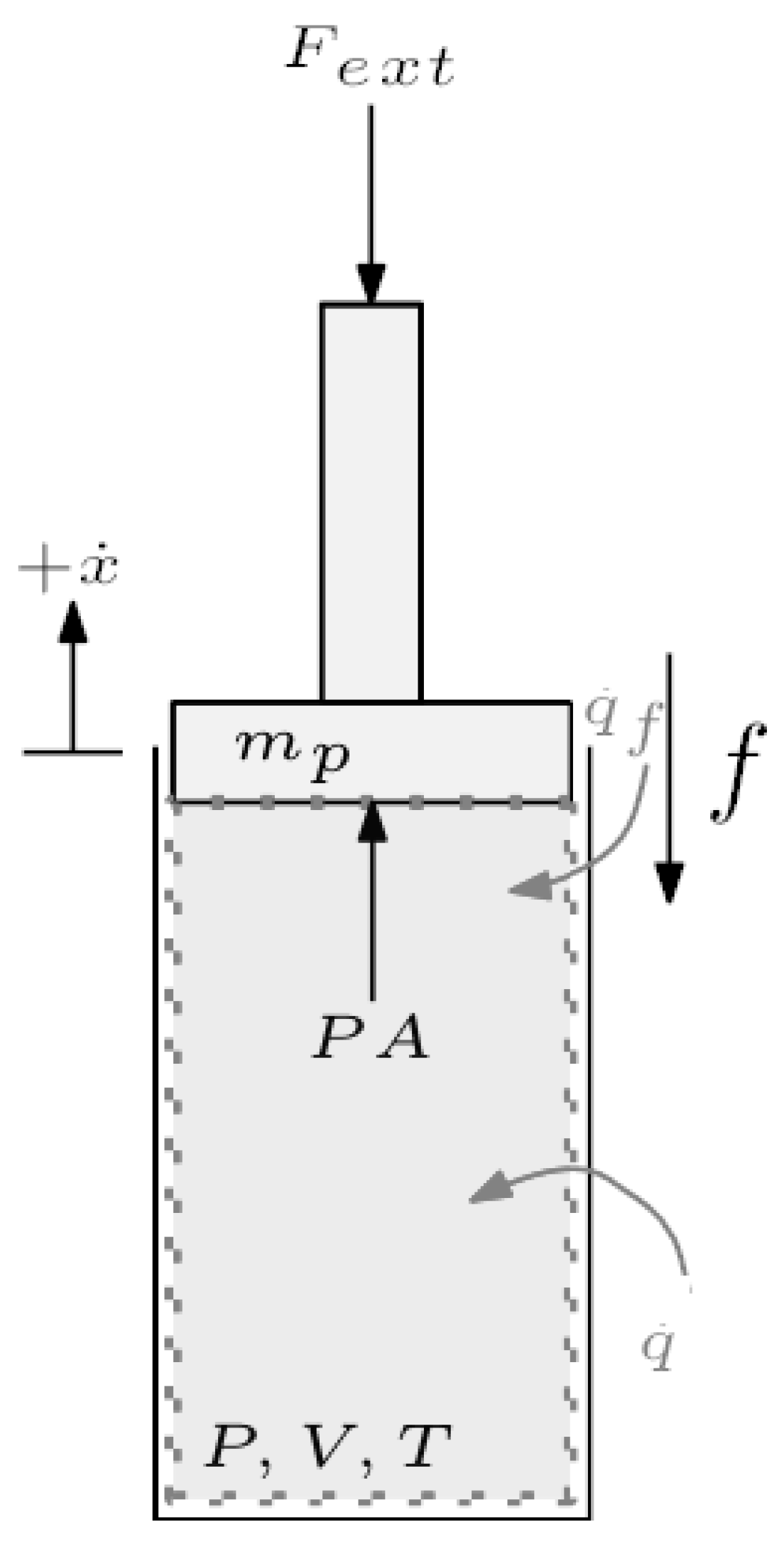
5. Optimal Control of an Electromechanical System
5.1. Case A: Load Power Transfer Optimization
5.1.1. Subsystem Definition and ECD
5.1.2. Objective Function
5.1.3. Optimal Control Problem Formulation
5.1.4. OCP Solution
5.1.5. Linear Friction Case
5.1.6. Solutions for vs. Sign of and Stability
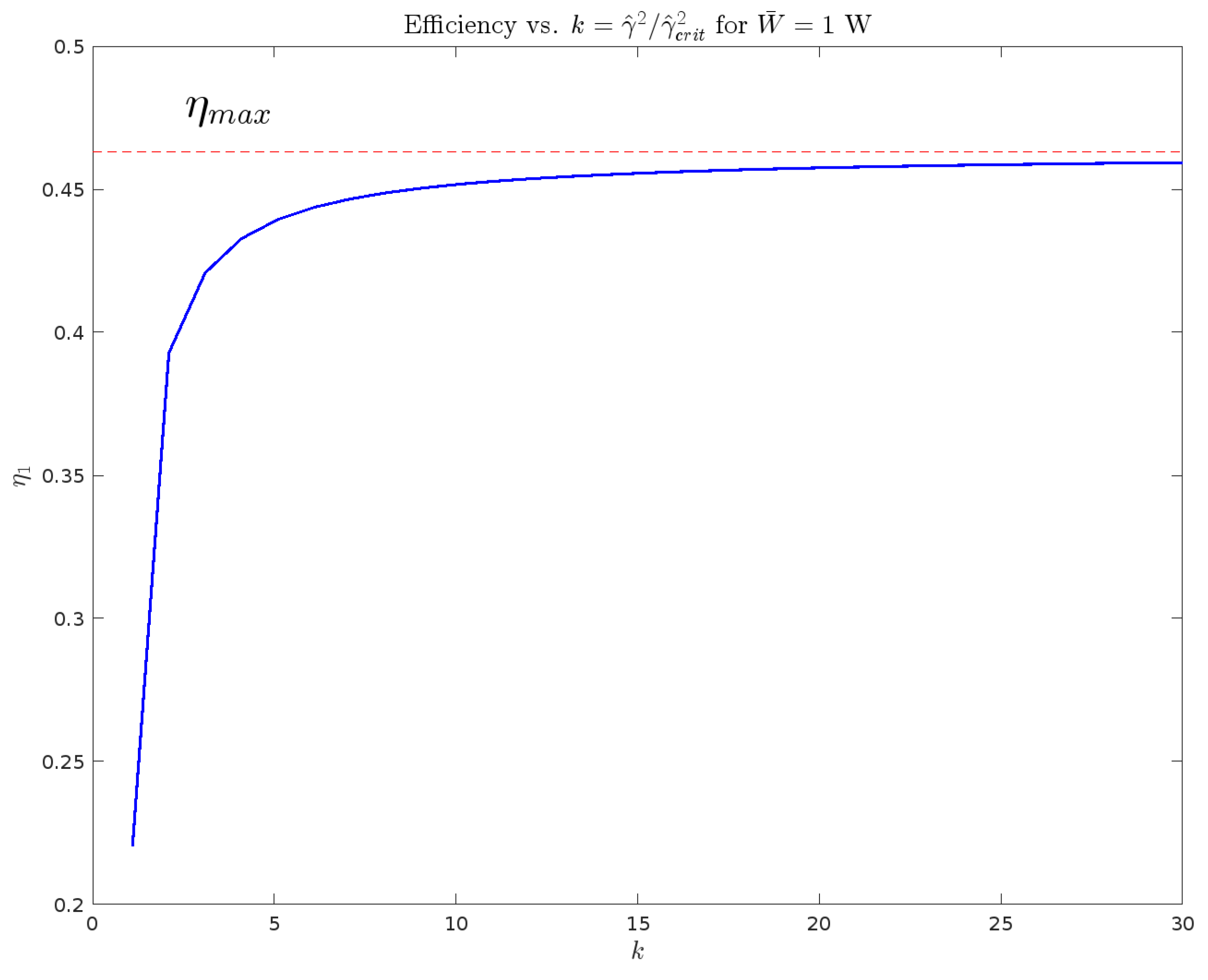
5.1.7. Efficiency
5.1.8. Maximal Efficiency Under EGM
5.2. Case B: Energy Harvesting Optimization
5.2.1. Subsystem Definition and ECD
5.2.2. Objective Function
5.2.3. OCP Formulation
5.2.4. OCP Solution
5.2.5. Solutions for vs. Sign of and Stability
5.2.6. Maximal Efficiency
5.3. Comparison with Efficiency Maximization
5.4. Summary
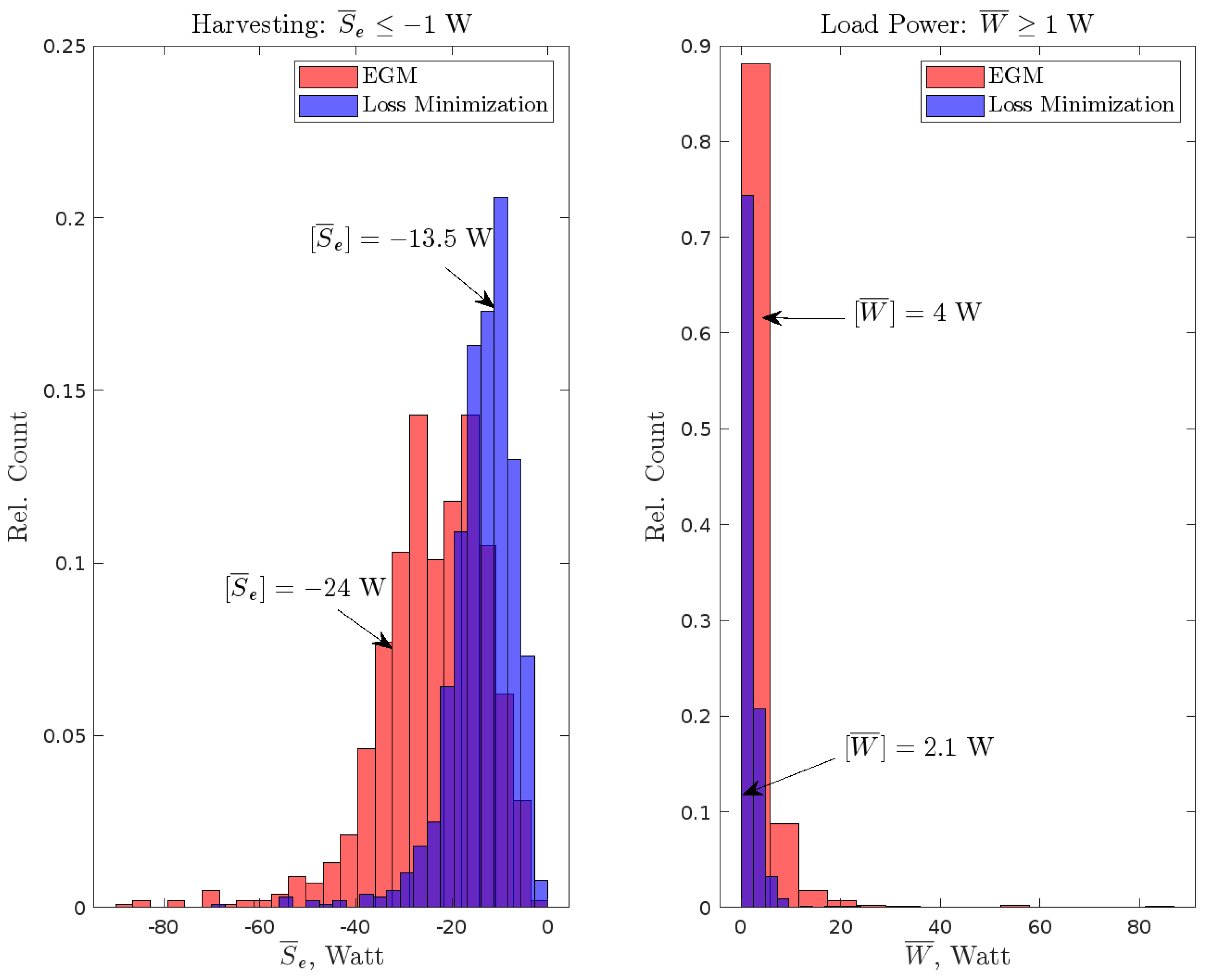
6. Numerical Simulation
Montecarlo Study with Inequality Constraints
7. Discussion
Author Contributions
Funding
Institutional Review Board Statement
Data Availability Statement
Conflicts of Interest
References
- Mai, T.; Hand, M.M.; Baldwin, S.F.; Wiser, R.H.; Brinkman, G.L.; Denholm, P.; Arent, D.J.; Porro, G.; Sandor, D.; Hostick, D.J.; et al. Renewable Electricity Futures for the United States. IEEE Trans. Sustain. Energy 2014, 5, 372–378. [Google Scholar] [CrossRef]
- What Is U.S. Electricity Generation by Energy Source? Available online: https://www.eia.gov/tools/faqs/faq.php?id=427&t=3 (accessed on 29 July 2024).
- Haddad, W. Thermodynamics: The Unique Universal Science. Entropy 2017, 19, 621. [Google Scholar] [CrossRef]
- Richter, H. Energy Cyclo-Directionality, Average Equipartition and Exergy Efficiency of Multidomain Power Networks. IEEE Control Syst. Lett. 2022, 6, 3337–3342. [Google Scholar] [CrossRef]
- Onsager, L. Reciprocal relations in irreversible processes. I. Phys. Rev. 1931, 37, 405. [Google Scholar] [CrossRef]
- Meixner, J. Thermodynamics of Electrical Networks and the Onsager-Casimir Reciprocal Relations. J. Math. Phys. 1963, 4, 154–159. [Google Scholar] [CrossRef]
- Flower, J.; Evans, F. Irreversible thermodynamics and stability considerations of electrical networks. J. Frankl. Inst. 1971, 291, 121–136. [Google Scholar] [CrossRef]
- Demirel, Y.; Gerbaud, V. Chapter 3—Fundamentals of Nonequilibrium Thermodynamics. In Nonequilibrium Thermodynamics, 4th ed.; Demirel, Y., Gerbaud, V., Eds.; Elsevier: Amsterdam, The Netherlands, 2019; pp. 135–186. [Google Scholar]
- Delvenne, J.C.; Sandberg, H.; Doyle, J. Thermodynamics of linear systems. In Proceedings of the European Control Conference (ECC), Online, 2–5 July 2007; pp. 840–847. [Google Scholar]
- Valencia-Ortega, G.; Arias-Hernandez, L. Thermodynamic Optimization of an Electric Circuit as a Non-steady Energy Converter. J. Non-Equilib. Thermodyn. 2017, 42, 187–199. [Google Scholar] [CrossRef]
- Gromov, D.; Caines, P. Interconnection of Thermodynamic Control Systems. In Proceedings of the IFAC World Congress, Milan, Italy, 28 August–2 September 2011; pp. 6091–6097. [Google Scholar]
- Berg, J.; Maithripala, D.; Hui, Q.; Haddad, W. Thermodynamics-Based Control of Network Systems. J. Dyn. Syst. Meas. Control 2013, 135, 051003. [Google Scholar] [CrossRef]
- Nash, A.; Jain, N. Second Law Modeling and Robust Control for Thermal-Fluid Systems. In Proceedings of the Dynamic Systems and Control Conference, Atlanta, GA, USA, 30 September–3 October 2018. [Google Scholar]
- Berg, J.; Maithripala, D.; Hui, Q.; Haddad, W. Thermodynamics-based network systems control by thermal analogy. In Proceedings of the IEEE 51st IEEE Conference on Decision and Control (CDC), Maui, HI, USA, 10–13 December 2012; pp. 3910–3915. [Google Scholar]
- Zeng, X.; Liu, Z.; Hui, Q. Energy Equipartition Stabilization and Cascading Resilience Optimization for Geospatially Distributed Cyber-Physical Network Systems. IEEE Trans. Syst. Man Cybern. Syst. 2015, 45, 25–43. [Google Scholar] [CrossRef]
- Lopez-Gonzalez, H.; Hernandez-Martinez, E.G.; de Portillo-Velez, R.; Ferreira-Vazquez, E.D.; Flores-Godoy, J.J.; Fernandez-Anaya, G. Formation Control for Thermal Multi-agent Systems. In Proceedings of the IEEE URUCON, Montevideo, Uruguay, 24–26 November 2021; pp. 390–394. [Google Scholar]
- Baros, S. A novel ectropy-based control scheme for a DFIG driven by a wind turbine with an integrated energy storage. In Proceedings of the American Control Conference (ACC), Chicago, IL, USA, 1–3 July 2015; pp. 4345–4351. [Google Scholar] [CrossRef]
- Cvetkovic, M.; Ilic, M. Ectropy-based nonlinear control of FACTS for transient stabilization. In Proceedings of the IEEE Power Energy Society General Meeting, Denver, CO, USA, 26–30 July 2015; p. 1. [Google Scholar]
- Haddad, W.M. A Dynamical Systems Theory of Thermodynamics; Princeton University Press: Princeton, NJ, USA, 2019. [Google Scholar]
- Haddad, W.; Nersesov, S.; Chellaboina, V. Heat flow, work energy, chemical reactions, and thermodynamics: A dynamical systems perspective. In Proceedings of the 2010 American Control Conference, Baltimore, MD, USA, 30 June–2 July 2010; pp. 1196–1203. [Google Scholar]
- Nersesov, S.; Haddad, W. Reversibility and Poincaré Recurrence in Linear Dynamical Systems. IEEE Trans. Autom. Control 2008, 53, 2160–2165. [Google Scholar] [CrossRef]
- van der Schaft, A. Classical Thermodynamics Revisited: A Systems and Control Perspective. IEEE Control Syst. Mag. 2021, 41, 32–60. [Google Scholar] [CrossRef]
- van der Schaft, A. Cyclo-Dissipativity Revisited. IEEE Trans. Autom. Control 2021, 66, 2920–2924. [Google Scholar] [CrossRef]
- van der Schaft, A. Cyclo-Dissipativity and Thermodynamics. In Proceedings of the 21st IFAC World Congress (Virtual), Berlin, Germany, 12–17 July 2020. [Google Scholar]
- van der Schaft, A.; Jeltsema, D. Limits to Energy Conversion. IEEE Trans. Autom. Control 2022, 67, 532–538. [Google Scholar] [CrossRef]
- Gouy, M. Sur l’énergie utilisable. J. Phys. Theor. Appl. 1889, 8, 501–518. [Google Scholar] [CrossRef]
- Lucia, U. The Gouy-Stodola theorem as a variational principle for open systems. Atti Della Accad. Peloritana Pericolanti-Cl. Sci. Fis. Mat. Nat. 2016, 94, 1–16. [Google Scholar]
- Bejan, A. Entropy Generation Minimization: The Method of Thermodynamic Optimization of Finite-Size Systems and Finite-Time Processes; Mechanical and Aerospace Engineering Series; CRC Press: Boca Raton, FL, USA, 1995. [Google Scholar]
- Jain, N.; Alleyne, A. Exergy-based optimal control of a vapor compression system. Energy Convers. Manag. 2015, 92, 353–365. [Google Scholar] [CrossRef]
- Teh, K.; Edwards, C. An Optimal Control Approach to Minimizing Entropy Generation in an Adiabatic Internal Combustion Engine. J. Dyn. Syst. Meas. Control 2008, 130, 19–27. [Google Scholar] [CrossRef]
- Haseli, Y. Interpretation of Entropy Calculations in Energy Conversion Systems. Energies 2021, 14, 7022. [Google Scholar] [CrossRef]
- Fathizadeh, M.; Richter, H. Thermodynamics-inspired trajectory optimization of a planar robotic arm. In Proceedings of the American Control Conference, Denver, CO, USA, 7–10 July 2025. [Google Scholar]
- Richter, H. Thermodynamic H∞ Control of Multidomain Power Networks. IEEE Control Syst. Lett. 2023, 7, 1939–1944. [Google Scholar] [CrossRef]
- Fathizadeh, M.; Richter, H. Efficiency Optimization of a Two-link Planar Robotic Arm. arXiv 2024, arXiv:2410.21185. [Google Scholar]
- Sangi, R.; Müller, D. Application of the second law of thermodynamics to control: A review. Energy 2019, 174, 938–953. [Google Scholar] [CrossRef]
- Green, M.; Limebeer, D. Linear Robust Control; Prentice-Hall: Englewood Cliffs, NJ, USA, 1995. [Google Scholar]
- Svoboda, J.; Dorf, R. Introduction to Electric Circuits; John Wiley & Sons: Hoboken, NJ, USA, 2014. [Google Scholar]


| Load Power | Harvesting | |||
|---|---|---|---|---|
| Criterion | EGM | Losses | EGM | Losses |
| Stability | ||||
| Obj. Feasibility | ||||
| Max. Efficiency | 1/2 | 1 | 1/2 | 1 |
| Parameter | Symbol | Value | Units |
|---|---|---|---|
| Mass | m | 0.1 | kg |
| Inductance | L | 1 | mH |
| Friction coefficient | b | 0.1 | |
| Resistance | R | 10 | |
| Conversion constant | 5 |
Disclaimer/Publisher’s Note: The statements, opinions and data contained in all publications are solely those of the individual author(s) and contributor(s) and not of MDPI and/or the editor(s). MDPI and/or the editor(s) disclaim responsibility for any injury to people or property resulting from any ideas, methods, instructions or products referred to in the content. |
© 2025 by the authors. Licensee MDPI, Basel, Switzerland. This article is an open access article distributed under the terms and conditions of the Creative Commons Attribution (CC BY) license (https://creativecommons.org/licenses/by/4.0/).
Share and Cite
Richter, H.; Fathizadeh, M.; Kaptain, T. Entropy Generation Optimization in Multidomain Systems: A Generalized Gouy-Stodola Theorem and Optimal Control. Entropy 2025, 27, 612. https://doi.org/10.3390/e27060612
Richter H, Fathizadeh M, Kaptain T. Entropy Generation Optimization in Multidomain Systems: A Generalized Gouy-Stodola Theorem and Optimal Control. Entropy. 2025; 27(6):612. https://doi.org/10.3390/e27060612
Chicago/Turabian StyleRichter, Hanz, Meysam Fathizadeh, and Tyler Kaptain. 2025. "Entropy Generation Optimization in Multidomain Systems: A Generalized Gouy-Stodola Theorem and Optimal Control" Entropy 27, no. 6: 612. https://doi.org/10.3390/e27060612
APA StyleRichter, H., Fathizadeh, M., & Kaptain, T. (2025). Entropy Generation Optimization in Multidomain Systems: A Generalized Gouy-Stodola Theorem and Optimal Control. Entropy, 27(6), 612. https://doi.org/10.3390/e27060612