


Does Excellence Correspond to Universal Inequality Level?


 and
and
Abstract
1. Introduction
2. Methods
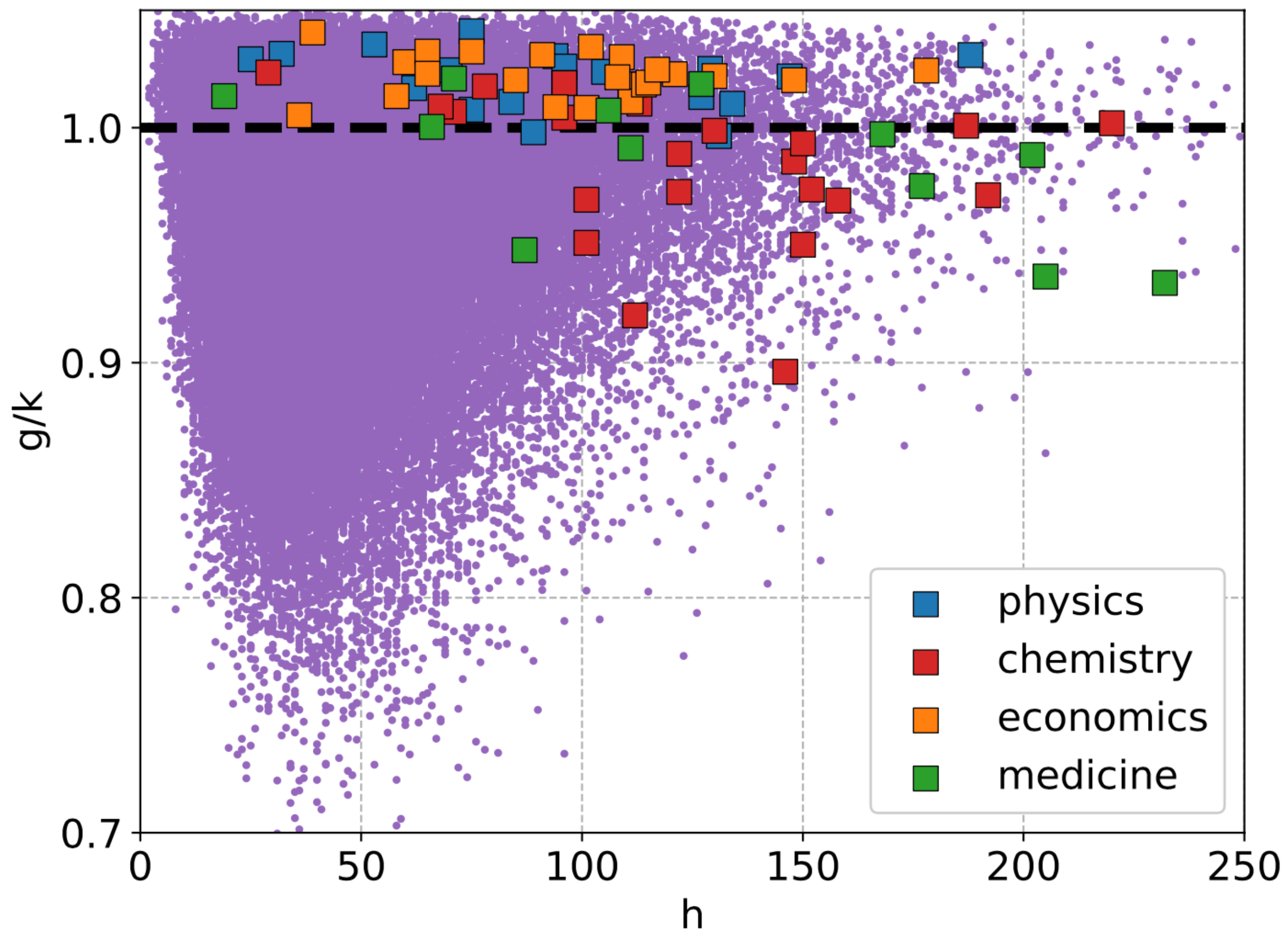
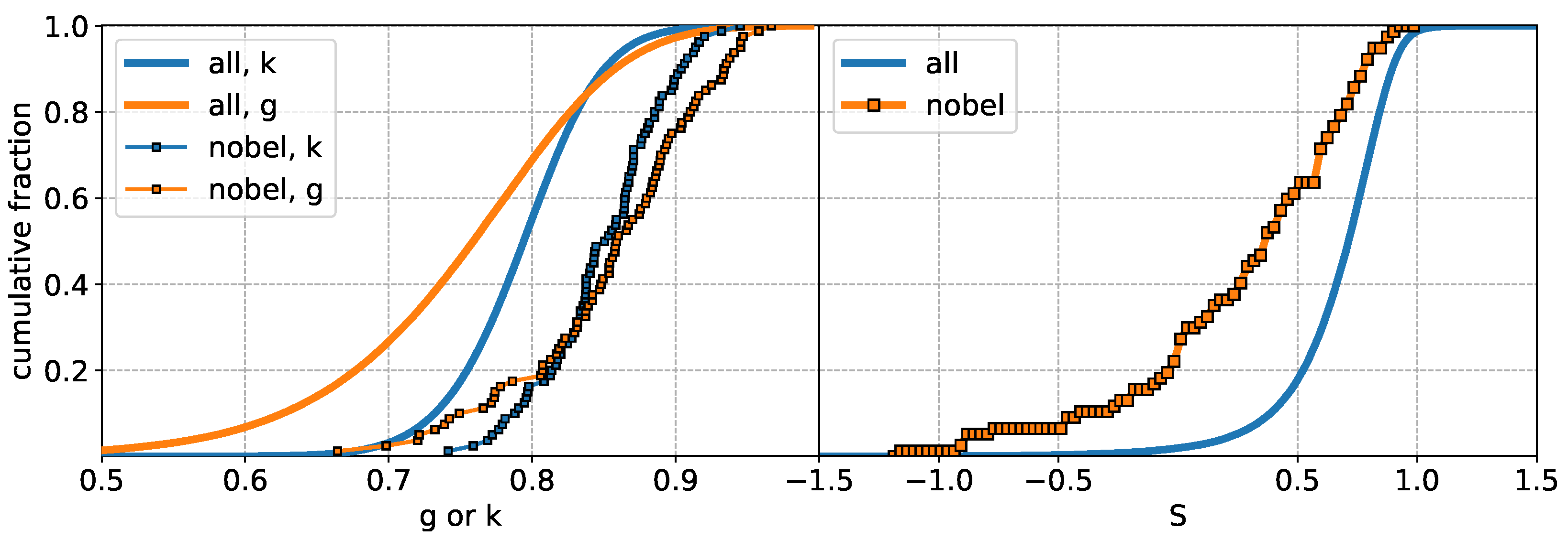
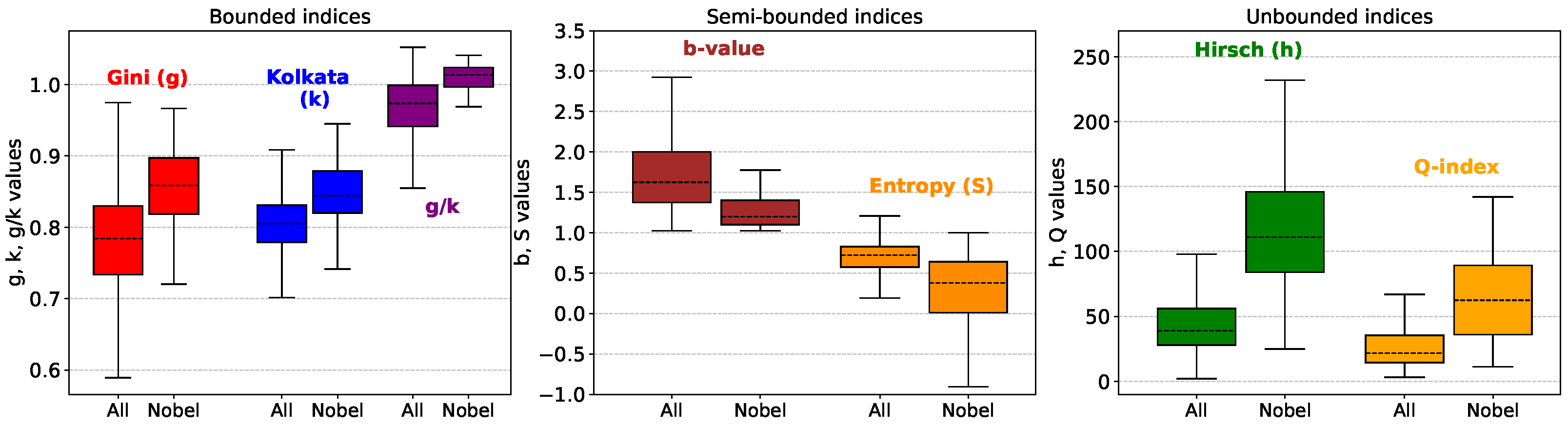
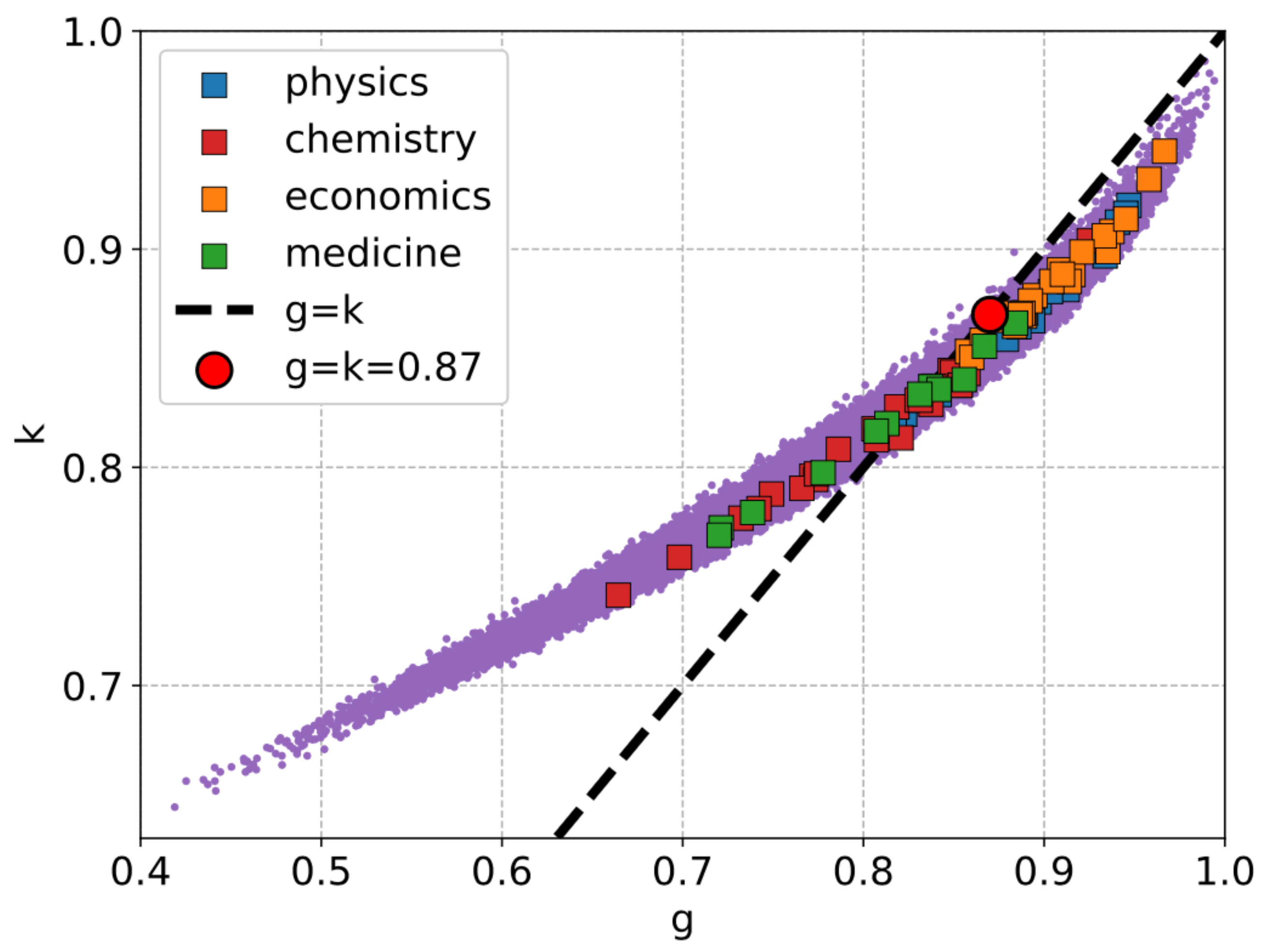
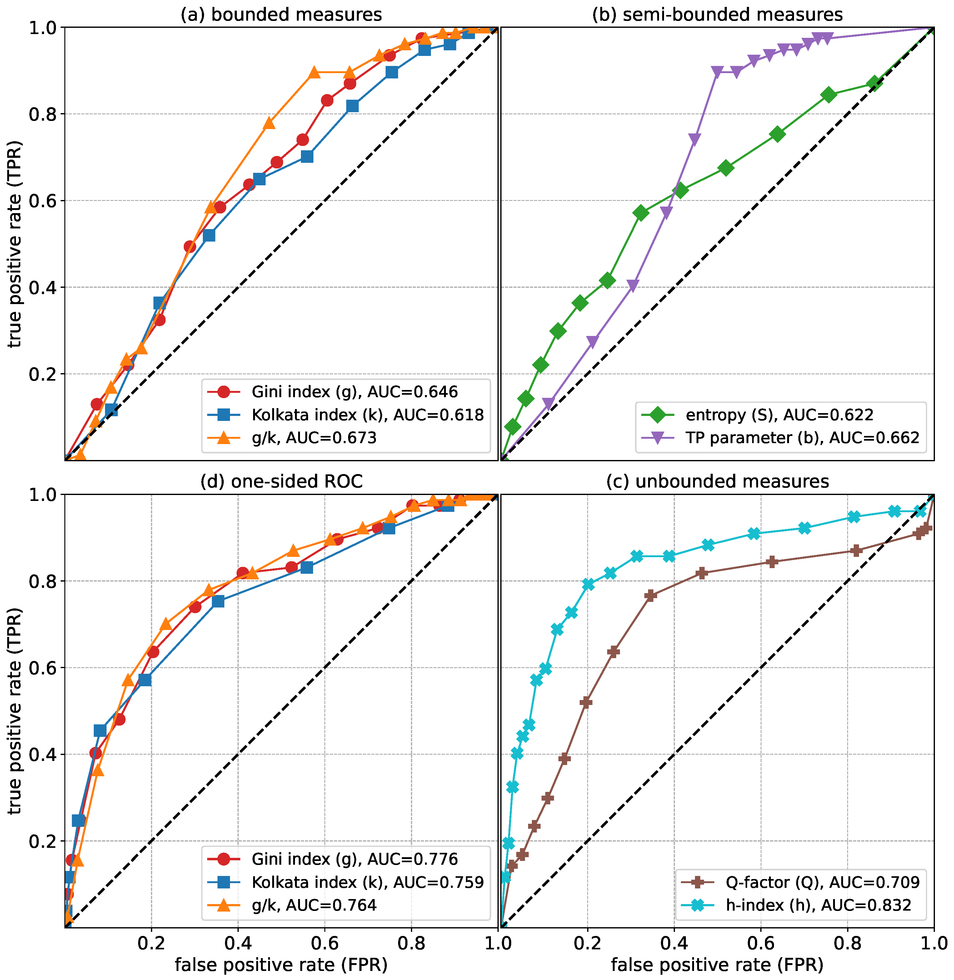
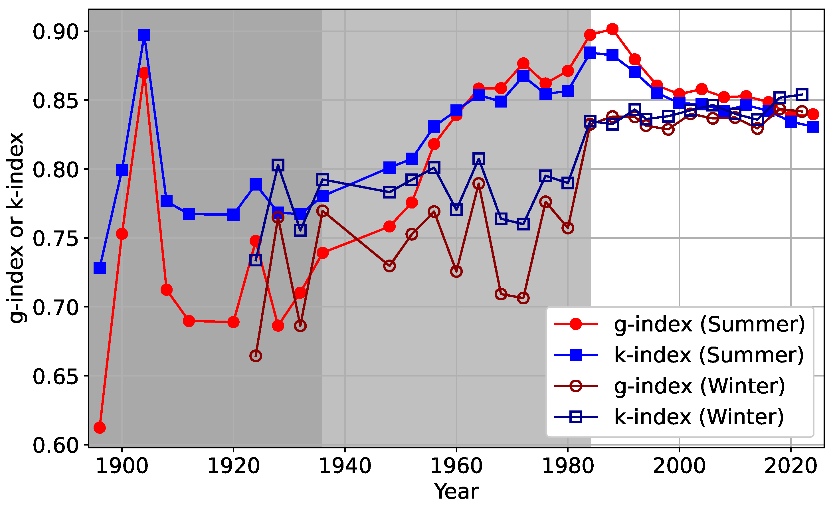
3. Results
3.1. Inequality in Citations

3.2. Inequality in Olympic Medals
4. Discussions and Conclusions
Author Contributions
Funding
Institutional Review Board Statement
Data Availability Statement
Conflicts of Interest
Abbreviations
| SOC | Self-Organized Criticality |
| ROC | Receiver Operation Characteristic |
| AUC | Area Under the Curve |
| TPR | True Positive Rate |
| FPR | False Positive Rate |
| TP | Tsallis-Pareto |
Appendix A

| Name | Year | Sub. | NP | NC | h | Q | g | k |
|---|---|---|---|---|---|---|---|---|
| Alain Aspect | 2022 | phys | 757 | 40,141 | 75 | 122.893 | 0.9337 | 0.8969 |
| Anne L Huillier | 2023 | phys | 504 | 34,777 | 84 | 77.1796 | 0.8469 | 0.8377 |
| Anton Zeilinger | 2022 | phys | 1098 | 113,609 | 147 | 71.3036 | 0.8897 | 0.8707 |
| Ardem Patapoutian | 2021 | med | 184 | 50,057 | 87 | 11.2758 | 0.7387 | 0.7793 |
| Benjamin List | 2021 | chem | 337 | 48,209 | 101 | 28.4021 | 0.7492 | 0.7878 |
| Carolyn R. Bertozzi | 2022 | chem | 1000 | 97,852 | 150 | 37.1544 | 0.8072 | 0.8126 |
| Daron Acemoglu | 2024 | eco | 1268 | 256,141 | 178 | 94.1268 | 0.9101 | 0.8885 |
| David Baker | 2024 | chem | 2503 | 184,477 | 220 | 62.2481 | 0.8388 | 0.8372 |
| David Card | 2021 | eco | 663 | 99,436 | 114 | 43.0442 | 0.8924 | 0.8763 |
| David W.C. MacMillan | 2021 | chem | 560 | 81,172 | 130 | 62.8993 | 0.8297 | 0.8308 |
| Demis Hassabis | 2024 | chem | 162 | 194,682 | 96 | 28.6888 | 0.8480 | 0.8444 |
| Emmanuelle Charpentier | 2020 | chem | 269 | 59,389 | 62 | 94.3811 | 0.9315 | 0.9012 |
| Ferenc Krausz | 2023 | phys | 1117 | 87,620 | 129 | 86.0893 | 0.8860 | 0.8644 |
| Gary Ruvkun | 2024 | med | 343 | 71,629 | 111 | 34.5301 | 0.8130 | 0.8201 |
| Geoffrey Hinton | 2024 | phys | 724 | 905,074 | 188 | 138.225 | 0.9406 | 0.9124 |
| Giorgio Parisi | 2021 | phys | 1115 | 108,250 | 134 | 117.507 | 0.8419 | 0.8334 |
| Guido W. Imbens | 2021 | eco | 348 | 110,070 | 101 | 26.0981 | 0.8747 | 0.8674 |
| James Robinson | 2024 | eco | 808 | 123,197 | 102 | 123.98 | 0.9452 | 0.9138 |
| Jennifer A. Doudna | 2020 | chem | 841 | 143,756 | 159 | 121.594 | 0.8586 | 0.8431 |
| John F. Clauser | 2022 | phys | 133 | 21,317 | 32 | 64.0487 | 0.9452 | 0.9164 |
| John Hopfield | 2024 | phys | 303 | 92,855 | 94 | 93.1922 | 0.8936 | 0.8672 |
| John Jumper | 2024 | chem | 72 | 58,763 | 29 | 40.8523 | 0.9250 | 0.9038 |
| Joshua D. Angrist | 2021 | eco | 400 | 101,784 | 91 | 107.176 | 0.9159 | 0.8884 |
| Katalin Kariko | 2023 | med | 222 | 29,678 | 66 | 20.0473 | 0.8373 | 0.8350 |
| Michael Houghton | 2020 | med | 533 | 60,722 | 106 | 89.2609 | 0.8418 | 0.8357 |
| Morten Meldal | 2022 | chem | 409 | 31,525 | 68 | 136.415 | 0.8208 | 0.8135 |
| Moungi G. Bawendi | 2023 | chem | 971 | 173,369 | 187 | 71.702 | 0.8315 | 0.8308 |
| Paul R. Milgrom | 2020 | eco | 383 | 116,246 | 85 | 41.2521 | 0.9085 | 0.8905 |
| Robert B. Wilson | 2020 | eco | 285 | 35,042 | 58 | 41.9753 | 0.8824 | 0.8707 |
| Simon Johnson | 2024 | eco | 849 | 90,468 | 65 | 178.742 | 0.9666 | 0.9449 |
| Svante Paabo | 2022 | med | 581 | 144,899 | 177 | 66.567 | 0.7777 | 0.7975 |
| Syukuro Manabe | 2021 | phys | 290 | 48,232 | 89 | 36.7611 | 0.8228 | 0.8244 |
| Victor Ambros | 2024 | med | 180 | 71,607 | 71 | 47.1312 | 0.8842 | 0.8661 |
| Year | Participating Countries | Total Medals | h | Q | g | k |
|---|---|---|---|---|---|---|
| 1896 | 14 | 122 | 6 | 5.78 | 0.6124 | 0.7283 |
| 1900 | 26 | 284 | 6 | 10.65 | 0.7530 | 0.7992 |
| 1904 | 12 | 280 | 4 | 11.51 | 0.8696 | 0.8973 |
| 1908 | 22 | 324 | 8 | 10.36 | 0.7124 | 0.7766 |
| 1912 | 28 | 317 | 8 | 5.95 | 0.6898 | 0.7672 |
| 1920 | 29 | 449 | 11 | 6.35 | 0.6890 | 0.7669 |
| 1924 | 44 | 392 | 10 | 11.36 | 0.7478 | 0.7888 |
| 1928 | 46 | 356 | 10 | 7.39 | 0.6864 | 0.7684 |
| 1932 | 37 | 370 | 10 | 11.30 | 0.7103 | 0.7672 |
| 1936 | 49 | 422 | 12 | 11.97 | 0.7392 | 0.7803 |
| 1948 | 59 | 443 | 12 | 11.38 | 0.7583 | 0.8010 |
| 1952 | 69 | 459 | 11 | 11.59 | 0.7757 | 0.8074 |
| 1956 | 72 | 451 | 12 | 15.86 | 0.8180 | 0.8308 |
| 1960 | 83 | 461 | 10 | 18.77 | 0.8391 | 0.8425 |
| 1964 | 93 | 504 | 12 | 17.90 | 0.8583 | 0.8536 |
| 1968 | 112 | 527 | 13 | 22.94 | 0.8586 | 0.8489 |
| 1972 | 121 | 600 | 13 | 20.13 | 0.8766 | 0.8673 |
| 1976 | 92 | 613 | 12 | 18.96 | 0.8620 | 0.8543 |
| 1980 | 80 | 631 | 12 | 25.03 | 0.8712 | 0.8567 |
| 1984 | 140 | 688 | 13 | 35.66 | 0.8973 | 0.8844 |
| 1988 | 159 | 739 | 14 | 28.58 | 0.9015 | 0.8824 |
| 1992 | 169 | 815 | 16 | 23.36 | 0.8795 | 0.8703 |
| 1996 | 197 | 842 | 16 | 23.75 | 0.8605 | 0.8552 |
| 2000 | 199 | 927 | 16 | 20.06 | 0.8543 | 0.8477 |
| 2004 | 201 | 926 | 16 | 22.03 | 0.8579 | 0.8470 |
| 2008 | 204 | 958 | 16 | 23.97 | 0.8521 | 0.8423 |
| 2012 | 204 | 960 | 16 | 22.21 | 0.8528 | 0.8463 |
| 2016 | 207 | 972 | 17 | 25.89 | 0.8485 | 0.8421 |
| 2020 | 206 | 1080 | 17 | 21.66 | 0.8385 | 0.8343 |
| 2024 | 207 | 1044 | 15 | 25.10 | 0.8397 | 0.8307 |
| Year | Participating Countries | Total Medals | h | Q | g | k |
|---|---|---|---|---|---|---|
| 1924 | 16 | 49 | 4 | 5.55 | 0.6645 | 0.7339 |
| 1928 | 25 | 41 | 4 | 9.15 | 0.7649 | 0.8029 |
| 1932 | 17 | 42 | 3 | 4.86 | 0.6863 | 0.7555 |
| 1936 | 28 | 51 | 4 | 8.24 | 0.7696 | 0.7924 |
| 1948 | 28 | 74 | 6 | 5.30 | 0.7297 | 0.7832 |
| 1952 | 30 | 67 | 5 | 7.16 | 0.7527 | 0.7922 |
| 1956 | 32 | 72 | 6 | 7.11 | 0.7691 | 0.8010 |
| 1960 | 30 | 83 | 6 | 7.59 | 0.7257 | 0.7704 |
| 1964 | 36 | 103 | 7 | 8.74 | 0.7894 | 0.8074 |
| 1968 | 37 | 106 | 7 | 4.89 | 0.7093 | 0.7639 |
| 1972 | 35 | 105 | 6 | 5.33 | 0.7064 | 0.7600 |
| 1976 | 37 | 111 | 6 | 9.00 | 0.7762 | 0.7951 |
| 1980 | 37 | 115 | 6 | 7.40 | 0.7572 | 0.7898 |
| 1984 | 49 | 117 | 6 | 10.47 | 0.8324 | 0.8347 |
| 1988 | 57 | 138 | 7 | 11.98 | 0.8380 | 0.8325 |
| 1992 | 64 | 171 | 7 | 9.73 | 0.8378 | 0.8431 |
| 1994 | 67 | 183 | 8 | 9.52 | 0.8314 | 0.8362 |
| 1998 | 72 | 205 | 10 | 10.19 | 0.8287 | 0.8383 |
| 2002 | 77 | 237 | 9 | 11.70 | 0.8400 | 0.8426 |
| 2006 | 80 | 252 | 11 | 9.21 | 0.8367 | 0.8463 |
| 2010 | 82 | 258 | 10 | 11.76 | 0.8373 | 0.8400 |
| 2014 | 88 | 284 | 10 | 8.68 | 0.8294 | 0.8357 |
| 2018 | 92 | 307 | 12 | 11.69 | 0.8435 | 0.8517 |
| 2022 | 91 | 327 | 13 | 10.30 | 0.8417 | 0.8540 |
References
- Stauffer, D. Income Inequality in the 21st Century—A Biased Summary of Piketty’s Capital in the Twenty-First Century. Int. J. Mod. Phys. C 2016, 27, 1630001. [Google Scholar] [CrossRef]
- Pareto, V. Cours d’économie politique. Political Sci. Q. 1896, 11, 750–751. [Google Scholar]
- Dubinsky, A.J.; Hansen, R.W. Improving Marketing Productivity: The 80/20 Principle Revisited. Calif. Manag. Rev. 1982, 25, 96–105. [Google Scholar] [CrossRef]
- Woolhouse, M.; Dye, C.; Etard, J.; Smith, T.; Charlwood, J.; Garnett, G.; Hagan, P.; Hii, J.; Ndhlovu, P.; Quinnell, R.; et al. Heterogeneities in the Transmission of Infectious Agents: Implications for the Design of Control Programs. Proc. Natl. Acad. Sci. USA 1997, 94, 338. [Google Scholar] [CrossRef]
- Abeles, J.; Conway, D.J. The Gini Coefficient as a Useful Measure of Malaria Inequality Among Populations. Malar. J. 2020, 19, 444. [Google Scholar] [CrossRef]
- Manna, S.S.; Biswas, S.; Chakrabarti, B.K. Near Universal Values of Social Inequality Indices in Self-Organized Critical Models. Phys. A 2022, 596, 127121. [Google Scholar] [CrossRef]
- Banerjee, S.; Biswas, S.; Chakrabarti, B.K.; Challagundla, S.K.; Ghosh, A.; Guntaka, S.R.; Koganti, H.; Kondapalli, A.R.; Maiti, R.; Mitra, M.; et al. Evolutionary Dynamics of Social Inequality and Coincidence of Gini and Kolkata Indices under Unrestricted Competition. Int. J. Mod. Phys. C 2023, 34, 2350048. [Google Scholar] [CrossRef]
- Biró, T.S.; Andras, T.; Józsa, M.; Néda, Z. Gintropic Scaling of Scientometric Indexes. Phys. A Stat. Mech. Its Appl. 2023, 618, 128717. [Google Scholar] [CrossRef]
- Nielsen, M.W.; Andersen, J.P. Global citation inequality is on the rise. Proc. Natl. Acad. Sci. USA 2021, 118, e2012208118. [Google Scholar] [CrossRef]
- Dong, K.; Wu, J.; Wang, K. On the inequality of citation counts of all publications of individual authors. J. Inf. 2021, 15, 101203. [Google Scholar] [CrossRef]
- Teich, E.G.; Kim, J.Z.; Lynn, C.W.; Simon, S.C.; Klishin, A.A.; Szymula, K.P.; Srivastava, P.; Bassett, L.C.; Zurn, P.; Bassett, D.S.; et al. Citation inequity and gendered citation practices in contemporary physics. Nat. Phys. 2022, 18, 1161–1170. [Google Scholar] [CrossRef]
- Nettasinghe, B.; Alipourfard, N.; Krishnamurthy, V.; Lerman, K. Emergence of structural inequalities in scientific citation networks. arxiv 2021, arXiv:2103.10944. [Google Scholar]
- Crespo, J.A.; Li, Y.; Ruiz-Castillo, J. The measurement of the effect on citation inequality of differences in citation practices across scientific fields. PLoS ONE 2013, 8, e58727. [Google Scholar] [CrossRef]
- Kiesslich, T.; Beyreis, M.; Zimmermann, G.; Traweger, A. Citation inequality and the Journal Impact Factor: Median, mean, (does it) matter? Scientometrics 2021, 126, 1249–1269. [Google Scholar] [CrossRef]
- Banerjee, S.; Biswas, S.; Chakrabarti, B.K.; Ghosh, A.; Mitra, M. Sandpile Universality in Social Inequality: Gini and Kolkata Measures. Entropy 2023, 25, 735. [Google Scholar] [CrossRef]
- Ghosh, A.; Manna, S.S.; Chakrabarti, B.K. Q Factor: A Measure of Competition Between the Topper and the Average in Percolation and in Self-Organized Criticality. Phys. Rev. E 2024, 110, 014131. [Google Scholar] [CrossRef]
- Lorenz, M.O. Methods of Measuring the Concentration of Wealth. Publ. Am. Stat. Assoc. 1905, 9, 209. [Google Scholar] [CrossRef]
- Gini, C. Measurement of Inequality of Incomes. Econ. J. 1921, 31, 124. [Google Scholar] [CrossRef]
- Ghosh, A.; Chattopadhyay, N.; Chakrabarti, B.K. Inequality in Societies, Academic Institutions and Science Journals: Gini and k-Indices. Phys. A 2014, 410, 30. [Google Scholar] [CrossRef]
- Banerjee, S.; Chakrabarti, B.K.; Mitra, M.; Mutuswami, S. Inequality Measures: The Kolkata Index in Comparison With Other Measures. Front. Phys. 2020, 8, 562182. [Google Scholar] [CrossRef]
- Hardy, M. Pareto’s Law. Math. Intell. 2010, 32, 38. [Google Scholar] [CrossRef]
- Cui, L.; Lin, C.; Huang, X. Kinetic Modeling of Wealth Distribution with Saving Propensity, Earnings Growth, and Matthew Effect. Europhys. Lett. 2023, 143, 12002. [Google Scholar] [CrossRef]
- Lin, C.; Cui, L. Kinetic Modelling of Economic Markets with Individual and Collective Transactions. arXiv 2025, arXiv:2502.13735. [Google Scholar]
- Biró, T.S.; Néda, Z. Gintropy: Gini Index Based Generalization of Entropy. Entropy 2020, 22, 879. [Google Scholar] [CrossRef]
- Hirsch, J.E. An Index to Quantify an Individual’s Scientific Research Output. Proc. Natl. Acad. Sci. USA 2005, 102, 16569. [Google Scholar] [CrossRef]
- Alonso, S.; Cabrerizo, F.J.; Herrera-Viedma, E.; Herrera, F. h-Index: A review focused in its variants, computation and standardization for different scientific fields. J. Inf. 2009, 3, 273–289. [Google Scholar] [CrossRef]
- Bihari, A.; Tripathi, S.; Deepak, A. A review on h-index and its alternative indices. J. Inf. Sci. 2021, 49, 624–665. [Google Scholar] [CrossRef]
- Author Citation Data. Available online: https://figshare.com/articles/dataset/Data_for_article_i_Does_Excellence_Correspond_to_Universal_Inequality_Level_i_/28827314 (accessed on 19 April 2025).
- Winter Olympics Medal Tally. Available online: https://www.topendsports.com/events/winter/medal-tally/medal-tables.htm (accessed on 10 March 2025).
- Summer Olympics Medal Tally. Available online: https://www.olympics.com/en/olympic-games (accessed on 19 April 2025).
- Ghosh, A.; Chakrabarti, B.K. Do Successful Researchers Reach the Self-Organized Critical Point? Physics 2024, 6, 46–59. [Google Scholar] [CrossRef]
- Yong, A. A Critique of Hirsch’s Citation Index: A Combinatorial Fermi Problem. Not. Am. Math. Soc. 2014, 61, 1040–1050. [Google Scholar] [CrossRef]
- Tanner, W.P., Jr.; Swets, J.A. A Decision-Making Theory of Visual Detection. Psychol. Rev. 1954, 61, 401–409. [Google Scholar] [CrossRef]
- Fawcett, T. An Introduction to ROC Analysis. Pattern Recognit. Lett. 2006, 27, 861. [Google Scholar] [CrossRef]
- Sustainable Development Goals. Available online: https://sdgs.un.org/goals (accessed on 10 March 2025).
- Siudem, G.; Żogała-Siudem, B.; Cena, A.; Gagolewski, M. Three dimensions of scientific impact. Proc. Natl. Acad. Sci. USA 2020, 117, 13896–13900. [Google Scholar] [CrossRef] [PubMed]
- Bornmann, L.; Mutz, R.; Daniel, H.D. Are there better indices for evaluation purposes than the h index? A comparison of nine different variants of the h index using data from biomedicine. J. Am. Soc. Inf. Sci. Technol. 2008, 59, 830–837. [Google Scholar] [CrossRef]

Disclaimer/Publisher’s Note: The statements, opinions and data contained in all publications are solely those of the individual author(s) and contributor(s) and not of MDPI and/or the editor(s). MDPI and/or the editor(s) disclaim responsibility for any injury to people or property resulting from any ideas, methods, instructions or products referred to in the content. |
© 2025 by the authors. Licensee MDPI, Basel, Switzerland. This article is an open access article distributed under the terms and conditions of the Creative Commons Attribution (CC BY) license (https://creativecommons.org/licenses/by/4.0/).
Share and Cite
Biswas, S.; Chakrabarti, B.K.; Ghosh, A.; Ghosh, S.; Józsa, M.; Néda, Z. Does Excellence Correspond to Universal Inequality Level? Entropy 2025, 27, 495. https://doi.org/10.3390/e27050495
Biswas S, Chakrabarti BK, Ghosh A, Ghosh S, Józsa M, Néda Z. Does Excellence Correspond to Universal Inequality Level? Entropy. 2025; 27(5):495. https://doi.org/10.3390/e27050495
Chicago/Turabian StyleBiswas, Soumyajyoti, Bikas K. Chakrabarti, Asim Ghosh, Sourav Ghosh, Máté Józsa, and Zoltán Néda. 2025. "Does Excellence Correspond to Universal Inequality Level?" Entropy 27, no. 5: 495. https://doi.org/10.3390/e27050495
APA StyleBiswas, S., Chakrabarti, B. K., Ghosh, A., Ghosh, S., Józsa, M., & Néda, Z. (2025). Does Excellence Correspond to Universal Inequality Level? Entropy, 27(5), 495. https://doi.org/10.3390/e27050495