

Systems and Methods for Transformation and Degradation Analysis


Abstract
1. Introduction
2. Definitions
- Observable: a metric such as a physical property or performance indicator is observable if it can be sensed and measured directly.
- Phenomenological: characterized by observable phenomena, such as volume expansion.
- Transformation: a change in state quantified by the difference between the instantaneously observable time varying value of a non-monotonic transformation measure (or performance indicator) and its initial/reference value.
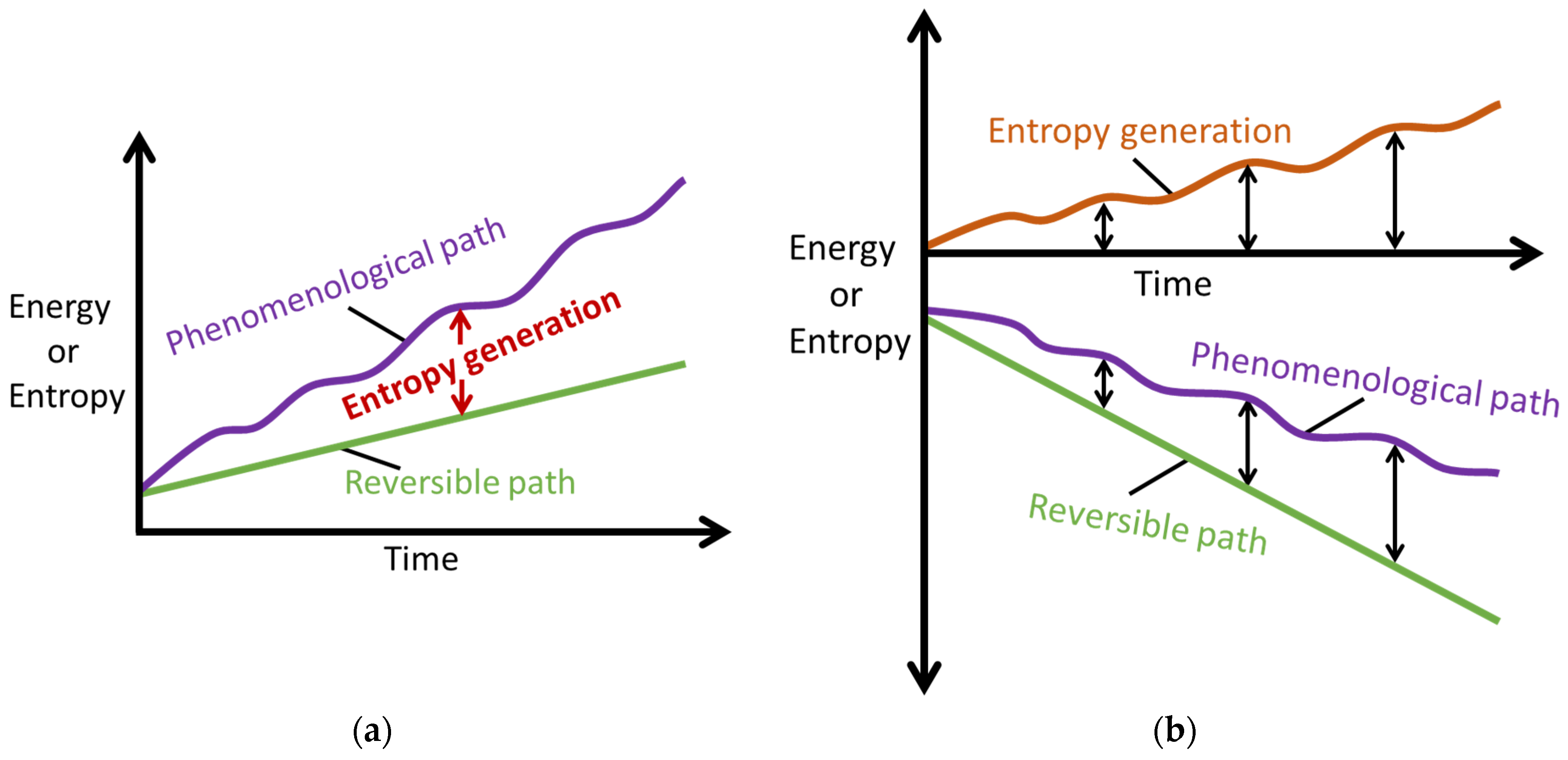
- Phenomenological transformation/degradation : the instantaneous transformation/degradation of a system or material via a non-monotonic transformation/degradation measure (or performance indicator).
- Phenomenological entropy generation : the instantaneous entropy generation along the transformation path through state space Z, observable through the state variables that characterize the active interactions, is always the sum of all active work and compositional change entropy generations and MST entropy [27]. Unlike entropy generation S′, which is always non-negative, is positive for energy addition and negative for energy extraction, in accordance with IUPAC sign convention.
- Reversible transformation : the idealized, quasi-static transformation of a system or material. can be estimated as the healthiest state transformation.
3. A Review of the Degradation–Entropy Generation Theorem
Statement
4. A Review of the Phenomenological Entropy Generation Theorem
4.1. Statement
4.2. Corollary
4.2.1. Heat and Work Lines—Instantaneous Orthogonality
4.2.2. Dissipation Factor J and Entropic Efficiency
5. Transformation–Phenomenological Entropy Generation Theorem
5.1. Reversible/Quasi-Static Transformation
5.2. Phenomenological Transformation
5.3. Phenomenological Transformation–Phenomenological Entropy Generation Theorem
6. Transformation/Degradation Analysis via TPEG Methods
Generalized Transformation Analysis Procedure
- (i)
- Identify a measurable transformation parameter, w, that is observable to the transformation characteristics;
- (ii)
- Measure or estimate the transformation , and evaluate the concurrent phenomenological entropy generation terms and due to the active processes during the interactions;
- (iii)
- Obtain the coefficients and by correlating transformation increments, accumulations or rates to phenomenological entropy generation increments, accumulation or rates (model calibration step);
- (iv)
- Re-combine the now-evaluated (or calibrated) coefficients with entropies and via Equation (15), to obtain instantaneous transformations in which were hitherto unobservable.
7. Transformation and Degradation Analysis Examples
7.1. Friction Sliding of Copper against Steel at Steady Speed—Steady State
7.2. Lubricants—Grease
7.3. Energy Storage Systems—Li-ion, Ni-MH, Pb-Acid Batteries, Supercapacitors and Fuel Cells
7.4. General Fatigue—Cyclic Bending and Torsion of Metal Rods
7.5. Pump Flow—Pressure and Flow Rate (Internal Energy)
8. Elements of the TPEG Methodology
8.1. PEG Terms: Work (Including Flow and Reaction) Entropy and MST/ECT Entropy
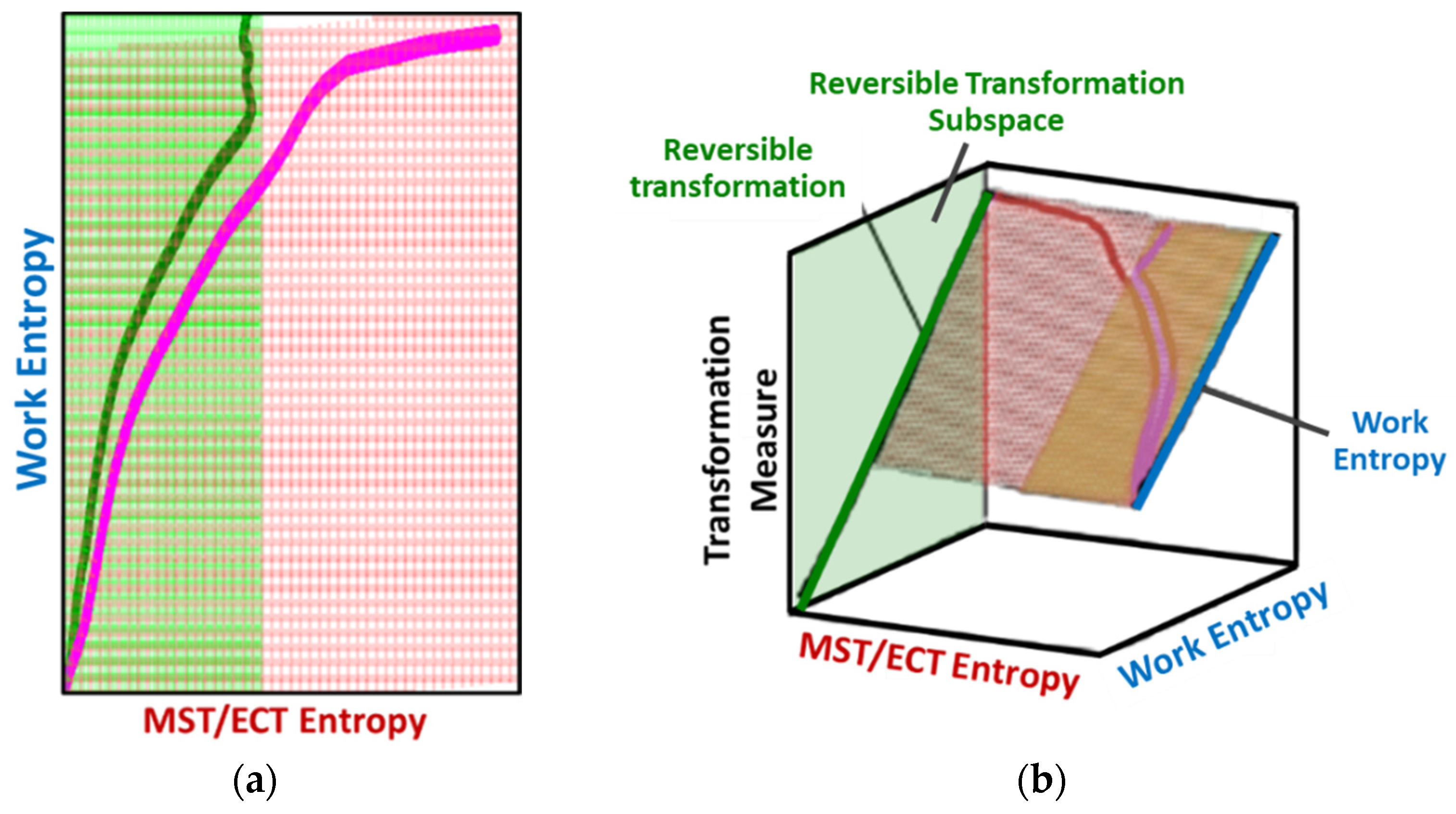
8.2. Degradation, A Geometric Problem: TPEG Trajectories, Hypersurfaces, and Domains
8.2.1. TPEG Coefficients
8.2.2. Entropy Generation Subspace and Reversible Transformation Subspace: Dissipation Factor J and Entropic Efficiency
9. Instability and Critical Phenomena
9.1. MST/ECT Entropy and Critical Failure Entropy
9.2. Thermal Runaway in Batteries
10. Discussion
11. Summary and Conclusions
Author Contributions
Funding
Institutional Review Board Statement
Data Availability Statement
Conflicts of Interest
Abbreviations
| Nomenclature | Name | Unit |
| A | chemical affinity | J/mol |
| B | DEG coefficient | Ah K/Wh |
| C | charge, charge transfer or capacity | Ah |
| charge fade or capacity fade | Ah | |
| F | Faraday’s constant | C/mol |
| G | Gibbs energy | Wh |
| I | discharge/charge current or rate | A |
| kB | Boltzmann constant | J/K |
| m | mass | kg |
| N | cycle number | |
| N, Nk | number of moles of substance | mol |
| p | dissipative process energy | J |
| P | pressure | Pa |
| q | charge | Ah |
| Q | heat | J |
| R | gas constant | J/mol·K |
| S | entropy or entropy content | Wh/K |
| S’ | entropy generation or production | Wh/K |
| t | time | s, min, h |
| T | temperature | degC or K |
| v | voltage | V |
| V | volume | m3 |
| w | degradation measure | |
| W | work | J |
| Symbols | ||
| μ | chemical potential | |
| ζ | phenomenological variable | |
| Subscripts and acronyms | ||
| Ω | Ohmic | |
| 0 | initial | |
| c, ch | charge | |
| d, disch | discharge | |
| f | final | |
| vT, ECT | ElectroChemicoThermal | |
| μT, MST | MicroStructuroThermal | |
| rev | reversible | |
| irr | irreversible | |
| phen | phenomenological | |
| DEG | degradation–entropy generation | |
| PEG | phenomenological entropy generation | |
| NLGI | National Lubricating Grease Institute |
References
- Osara, J.A. Thermodynamics of Manufacturing Processes—The Workpiece and the Machinery. Inventions 2019, 4, 28. [Google Scholar] [CrossRef]
- Bryant, M.D. Chapter 3: Thermodynamics of Ageing and Degradation in Engineering Devices and Machines. In The Physics of Degradation in Engineered Materials and Devices: Fundamentals and Principles; EBL-Schweitzer; Momentum Press: New York, NY, USA, 2014; ISBN 978-1-60650-468-0. [Google Scholar]
- Lemaitre, J.; Chaboche, J.L. Mechanics of Solid Materials; Cambridge University Press: New York, NY, USA, 1994; ISBN 978-0-521-47758-1. [Google Scholar]
- Bejan, A.; Tsatsaronis, G.; Moran, M.J. Thermal Design and Optimization; Wiley: New York, NY, USA, 1996. [Google Scholar]
- Bejan, A. Entropy Generation Minimization: The Method of Thermodynamic Optimization of Finite-Size Systems and Finite-Time Processes; Mechanical and Aerospace Engineering Series; CRC Press: Boca Raton, FL, USA, 2013; ISBN 978-1-4822-3917-1. [Google Scholar]
- Kuhn, E. An Energy Interpretation of Thixotropic Effects. Wear 1991, 142, 203–205. [Google Scholar] [CrossRef]
- Kuhn, E. Description of the Energy Level of Tribologically Stressed Greases. Wear 1995, 188, 138–141. [Google Scholar] [CrossRef]
- Naderi, M.; Khonsari, M.M. An Experimental Approach to Low-Cycle Fatigue Damage Based on Thermodynamic Entropy. Int. J. Solids Struct. 2010, 47, 875–880. [Google Scholar] [CrossRef]
- Amiri, M.; Naderi, M.; Khonsari, M.M. An Experimental Approach to Evaluate the Critical Damage. Int. J. Damage Mech. 2011, 20, 89–112. [Google Scholar] [CrossRef]
- Naderi, M.; Khonsari, M.M. A Comprehensive Fatigue Failure Criterion Based on Thermodynamic Approach. J. Compos. Mater. 2012, 46, 437–447. [Google Scholar] [CrossRef]
- Naderi, M.; Khonsari, M.M. Thermodynamic Analysis of Fatigue Failure in a Composite Laminate. Mech. Mater. 2012, 46, 113–122. [Google Scholar] [CrossRef]
- Rezasoltani, A.; Khonsari, M.M. On the Correlation between Mechanical Degradation of Lubricating Grease and Entropy. Tribol. Lett. 2014, 56, 197–204. [Google Scholar] [CrossRef]
- Rezasoltani, A.; Khonsari, M.M. An Engineering Model to Estimate Consistency Reduction of Lubricating Grease Subjected to Mechanical Degradation under Shear. Tribol. Int. 2016, 103, 465–474. [Google Scholar] [CrossRef]
- Aghdam, A.B.; Khonsari, M.M. Prediction of Wear in Grease-Lubricated Oscillatory Journal Bearings via Energy-Based Approach. Wear 2014, 318, 188–201. [Google Scholar] [CrossRef]
- Sosnovskiy, L.; Sherbakov, S. Surprises of Tribo-Fatigue; Magic Book: Minsk, Belarus, 2009. [Google Scholar]
- Sosnovskiy, L.A.; Sherbakov, S.S. Mechanothermodynamic Entropy and Analysis of Damage State of Complex Systems. Entropy 2016, 18, 268. [Google Scholar] [CrossRef]
- Basaran, C.; Nie, S. An Irreversible Thermodynamics Theory for Damage Mechanics of Solids. Int. J. Damage Mech. 2004, 13, 205–223. [Google Scholar] [CrossRef]
- Gomez, J.; Basaran, C. A Thermodynamics Based Damage Mechanics Constitutive Model for Low Cycle Fatigue Analysis of Microelectronics Solder Joints Incorporating Size Effects. Int. J. Solids Struct. 2005, 42, 3744–3772. [Google Scholar] [CrossRef]
- Basaran, C. Introduction to Unified Mechanics Theory with Applications; Springer International Publishing: Berlin/Heidelberg, Germany, 2023; ISBN 978-3-031-18621-9. [Google Scholar]
- Osara, J.; Bryant, M. A Thermodynamic Model for Lithium-Ion Battery Degradation: Application of the Degradation-Entropy Generation Theorem. Inventions 2019, 4, 23. [Google Scholar] [CrossRef]
- Osara, J.A.; Bryant, M.D. Performance and Degradation Characterization of Electrochemical Power Sources Using Thermodynamics. Electrochim. Acta 2021, 365, 137337. [Google Scholar] [CrossRef]
- Osara, J.A. Thermodynamics of Degradation; The University of Texas at Austin: Austin, TX, USA, 2017. [Google Scholar]
- Osara, J.A.; Bryant, M.D. Thermodynamics of Grease Degradation. Tribol. Int. 2019, 137, 433–445. [Google Scholar] [CrossRef]
- Osara, J.A.; Bryant, M.D. Thermodynamics of Fatigue: Degradation-Entropy Generation Methodology for System and Process Characterization and Failure Analysis. Entropy 2019, 21, 685. [Google Scholar] [CrossRef] [PubMed]
- Osara, J.A.; Bryant, M.D. A Temperature-Only System Degradation Analysis Based on Thermal Entropy and the Degradation-Entropy Generation Methodology. Int. J. Heat Mass Transf. 2020, 158, 120051. [Google Scholar] [CrossRef]
- Osara, J.A.; Bryant, M.D. Thermodynamics of Lead-Acid Battery Degradation: Application of the Degradation-Entropy Generation Methodology. J. Electrochem. Soc. 2019, 166, A4188. [Google Scholar] [CrossRef]
- Osara, J.A.; Bryant, M.D. Methods to Calculate Entropy Generation. Entropy 2024, 26, 237. [Google Scholar] [CrossRef]
- Bryant, M.D.; Khonsari, M.M.; Ling, F.F. On the Thermodynamics of Degradation. Proc. R. Soc. Math. Phys. Eng. Sci. 2008, 464, 2001–2014. [Google Scholar] [CrossRef]
- Moran, M.J.; Shapiro, H.N. Fundamentals of Engineering Thermodynamics, 5th ed.; Wiley: Hoboken NJ, USA, 2004. [Google Scholar]
- Kondepudi, D.; Prigogine, I. Modern Thermodynamics from Heat Engines to Dissipative Structures; John Wiley & Sons, Inc.: New York, NY, USA, 1998. [Google Scholar]
- Osara, J.A.; Ezekoye, O.A.; Marr, K.C.; Bryant, M.D. A Methodology for Analyzing Aging and Performance of Lithium-Ion Batteries: Consistent Cycling Application. J. Energy Storage 2021, 42, 103119. [Google Scholar] [CrossRef]
- Burghardt, M.D.; Harbach, J.A. Engineering Thermodynamics, 4th ed.; HarperCollins College Publishers: New York, NY, USA, 1993. [Google Scholar]
- Çengel, Y.A. Thermodynamics: An Engineering Approach, 6th ed.; McGraw-Hill Higher Education: Boston, MA, USA, 2008. [Google Scholar]
- Kuhn, E. Correlation between System Entropy and Structural Changes in Lubricating Grease. Lubricants 2015, 3, 332–345. [Google Scholar] [CrossRef]
- Lugt, P.M. Grease Lubrication in Rolling Bearings; John Wiley & Sons Ltd.: Hoboken, NJ, USA, 2013; ISBN 0824772040. [Google Scholar]
- Rincon, J.S.; Osara, J.; Bryant, M.D.; Fernández, B.R. Shannon’s Machine Capacity & Degradation-Degradation-Entropy Generation Methodologies for Failure Detection: Practical Applications to Motor-Pump Systems. In Proceedings of the 37th International Pump Users Symposium; Turbomachinery Laboratory, Texas A&M Engineering Experiment Station, Houston, TX, USA, 13 December 2021. [Google Scholar]
- Bryant, M.D.; Osara, J.A. On Degradation-Entropy Generation Theorems and Vector Spaces for Irreversible Thermodynamics. Appl. Mech. 2024. in submission. [Google Scholar]
- Feng, X.; Ouyang, M.; Liu, X.; Lu, L.; Xia, Y.; He, X. Thermal Runaway Mechanism of Lithium Ion Battery for Electric Vehicles: A Review. Energy Storage Mater. 2018, 10, 246–267. [Google Scholar] [CrossRef]
- Ouyang, M.; Ren, D.; Lu, L.; Li, J.; Feng, X.; Han, X.; Liu, G. Overcharge-Induced Capacity Fading Analysis for Large Format Lithium-Ion Batteries with LiyNi1/3Co1/3Mn1/3O2 + LiyMn2O4 Composite Cathode. J. Power Sources 2015, 279, 626–635. [Google Scholar] [CrossRef]
- Rohatgi, A. WebPlotDigitizer. Version 4.8. Available online: https://apps.automeris.io/wpd4/ (accessed on 25 March 2024).
- Bejan, A.; Kestin, J. Entropy Generation through Heat and Fluid Flow. J. Appl. Mech. 1983, 50, 475. [Google Scholar] [CrossRef]


| Work | |
|---|---|
| Frictional | |
| Magnetic | |
| Shear | |
| Electrical | |
| Rotational shaft | |
| Chemical | |
| Flow |
| # | Characterization Step | Model and Graphical Representation |
|---|---|---|
| (i) | Measured or input data | 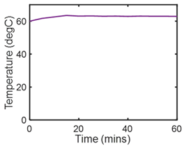 |
| (ii) | Phenomenological Entropy Generation Frictional entropy MST entropy | 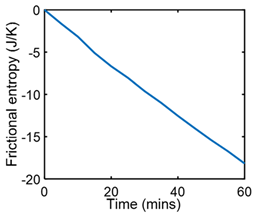 |
| (iii) | Degradation–Entropy Generation Material wear is the degradation measure. Slope yielded K/J | Degradation model:  |
| # | Characterization Step | Model and Graphical Representation |
|---|---|---|
| (i) | Measured or input data |  |
| (ii) | Phenomenological Entropy Generation MST entropy density Shear entropy density |  |
| (iii) | Transformation–Phenomenological Entropy Generation Shear stress accumulation is the trans-formation measure. Orthogonal slopes yielded Pa-s K/J for NLGI 4 grease. | Transformation model: 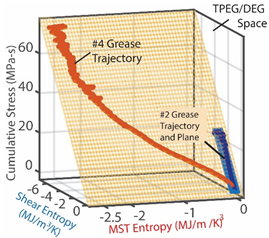 |
| (iv) | Change in shear strength/stress is the degradation measure. 0.396 |  |
| # | Characterization Step | Model and Graphical Representations |
|---|---|---|
| (i) | Measured or input data. |  |
| (ii) | Phenomenological Entropy Generation ECT entropy Ohmic entropy | 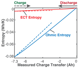 |
| (iii) | Transformation–Phenomenological Entropy Generation Charge content is the transformation measure. TPEG coefficients: Ah K/Wh and Ah K/Wh for discharge. For charge, Ah K/Wh and Ah K/Wh. | Transformation model:  |
| (iv) | Charge capacity fade is the degradation measure. For this cycle, Ah Ah 0.033 0.72 0.93 | Degradation model: 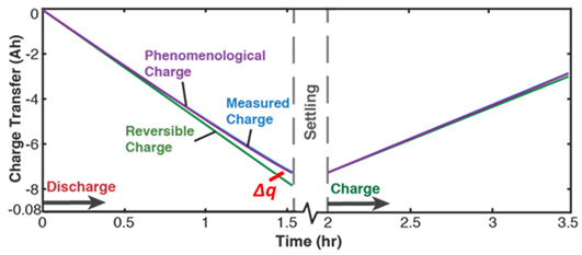 |
| # | Characterization Step | Model and Graphical Representation |
|---|---|---|
| (i) | Measured or input data |  |
| (ii) | Phenomenological Entropy Generation |  |
| (iii) | Transformation–Phenomenological Entropy Generation Strain is the transformation measure. Orthogonal slopes yielded %m3K/MJ and %m3K/MJ (bending), and %m3K/MJ and %m3K/MJ (torsion), prior to failure onset. | Transformation model: 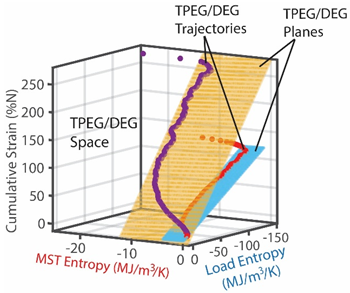 |
| (iv) | Change in strain is the degradation measure. At onset of failure, 0.10 |  |
| # | Characterization Step | Model and Graphical Representation |
|---|---|---|
| (i) | Measured or input data | 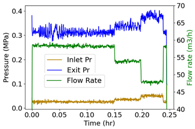 |
| (ii) | Phenomenological Entropy Generation Flow entropy Work entropy |  |
| (iii) | Transformation–Phenomenological Entropy Generation Pressure drop is the transformation measure. Orthogonal slopes give MPa-h K/kJ and MPa-h K/kJ | Transformation model: 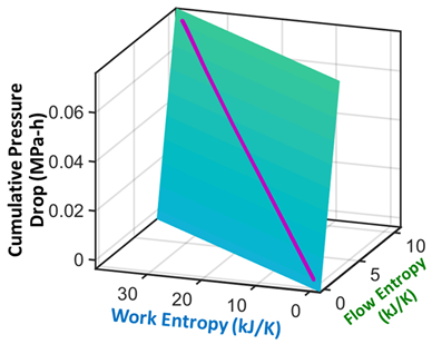 |
| (iv) | Change in pressure drop measures degradation. | 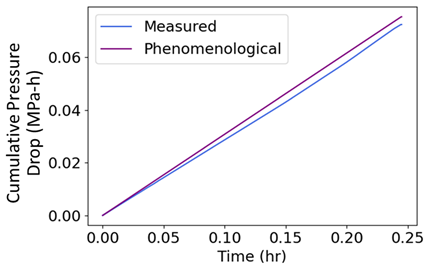 |
Disclaimer/Publisher’s Note: The statements, opinions and data contained in all publications are solely those of the individual author(s) and contributor(s) and not of MDPI and/or the editor(s). MDPI and/or the editor(s) disclaim responsibility for any injury to people or property resulting from any ideas, methods, instructions or products referred to in the content. |
© 2024 by the authors. Licensee MDPI, Basel, Switzerland. This article is an open access article distributed under the terms and conditions of the Creative Commons Attribution (CC BY) license (https://creativecommons.org/licenses/by/4.0/).
Share and Cite
Osara, J.A.; Bryant, M.D. Systems and Methods for Transformation and Degradation Analysis. Entropy 2024, 26, 454. https://doi.org/10.3390/e26060454
Osara JA, Bryant MD. Systems and Methods for Transformation and Degradation Analysis. Entropy. 2024; 26(6):454. https://doi.org/10.3390/e26060454
Chicago/Turabian StyleOsara, Jude A., and Michael D. Bryant. 2024. "Systems and Methods for Transformation and Degradation Analysis" Entropy 26, no. 6: 454. https://doi.org/10.3390/e26060454
APA StyleOsara, J. A., & Bryant, M. D. (2024). Systems and Methods for Transformation and Degradation Analysis. Entropy, 26(6), 454. https://doi.org/10.3390/e26060454