1. Introduction
Under the vision of “Internet of Everything”, intelligence-enabled applications are essential, leading to a variety of crucial computation tasks, such as the training and inference of complex machine learning models based on extensive datasets [
1,
2,
3]. However, executing these computation-intensive tasks on a single device with limited computation capability and power resources presents significant challenges. To this end, distributed computing emerges as a practical solution, where a central node, referred to as
master, manages task division, assignment, and result collection, while multiple distributed computing nodes, called
workers, process the assigned partial computation tasks in parallel [
4].
Nevertheless, while distributed computing accelerates the computation process by employing multiple workers for parallel processing, the total delay is dominated by the slowest worker, as the master must wait for all workers to complete their assigned tasks [
5]. As demonstrated in the experimental results of [
6], the delay of the slowest worker can exceed five times that of the others, which significantly prolongs the total delay. Moreover, due to the randomness of delays, identifying slow workers in advance is challenging. To tackle this so-called
straggling effect, coded computing has emerged as a promising solution [
6,
7,
8,
9,
10,
11,
12]. As
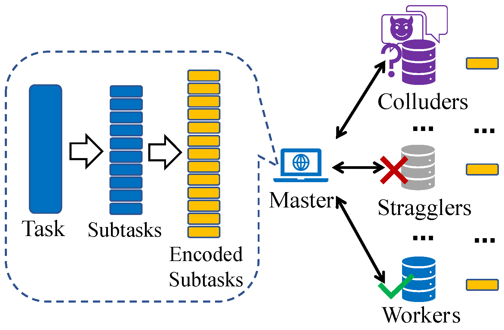
Figure 1 shows, this approach combines coding theory with distributed computing and reduces delays by introducing structured computational redundancies. Through the incorporation of redundancy during the encoding process, computation tasks can be completed using results from a subset of workers, thereby reducing total delays.
In coded computing, workers are tasked with processing input data and returning results, but the involved tasks may contain sensitive information, such as patient medical data, customer personal information, and proprietary company data [
13,
14]. Consequently, it is essential to maintain the data
privacy against colluding workers, those who return correct results but may communicate with one another to share input data from the master, so as to infer some private information of the master. Recent research studies have aimed to develop coded computing strategies that address not only the straggling effect but also privacy concerns, such as combining additional random data insertion with prevalent polynomial coded computing methods [
15,
16,
17,
18,
19,
20,
21,
22,
23,
24,
25]. This approach enhances the robustness of the system against straggling workers while also improving privacy and security by obscuring the original data.
In the majority of existing studies, matrix multiplication is treated as the primary application of coded computing, and its performance has been extensively validated. However, real-world computation tasks are often more diverse than mere matrix multiplication. For instance, in a linear regression task, the iterative process of solving weights involves calculating previous weights multiplied by the quadratic power of the input data. This implies that coded computing schemes for matrix multiplication must be executed twice in each step, and computation becomes considerably more complex when considering other tasks, such as inference tasks of neural networks.
In terms of extending the applicability of coded computing, one state-of-the-art approach is Lagrange Coded Computing (LCC) [
15]. LCC employs Lagrange polynomial interpolation to transform input data before and after encoding into interpolation points on the computation function. This allows the recovery of desired results through the reconstruction of the interpolation function. LCC is compatible with various computation tasks, ranging from matrix multiplication to polynomial functions, and offers an optimal recovery threshold concerning the degree of polynomial functions. In [
21,
25,
26], the problem of using matrix data as input and polynomial functions as computation tasks is also explored.
However, LCC still suffers from several shortcomings [
27]. First, its recovery threshold is proportional to degrees of polynomial functions, which can be prohibitively large for complex tasks and thereby make it difficult to achieve successful recovery. Second, Lagrange polynomial interpolation can be ill-conditioned, making it challenging to ensure numerical stability, unless one embeds the computation to a finite field. In [
27], Berrut’s Approximated Coded Computing (BACC) is proposed to address these shortcomings and further expand the scope of computation tasks to arbitrary functions. However, BACC only yields approximated computing results and does not guarantee privacy preservation. Other related works [
28,
29,
30,
31,
32] also focus on approximated results while attempting to maintain the numerical stability of coded computing. As far as we know, there is still a lack of a versatile coded computing strategy suitable for various computational tasks. This strategy should be capable of achieving privacy preservation while providing accurate or approximated results based on specific demands.
On the other hand, opportunities exist to enhance mitigation of the straggling effect and further reduce delays. This is because prior studies commonly discard results from straggling workers, leading to the inefficient utilization of computational resources. In [
11], a hierarchical task partitioning structure is proposed, where divided tasks are further partitioned into multiple layers, and workers process their assigned tasks in the order of layer indices. Consequently, straggling workers can return results from lower layers instead of none, while fast workers can reach higher layers and return more results. Similar performance improvements are achieved through multi-message communications (MMC) [
33,
34,
35], where workers are permitted to return partial results of assigned tasks in each time slot, enabling straggling workers to contribute to the system.
Essentially, three ways exist to alleviate the straggling effect, given the total number of workers. First, minimize the recovery threshold of coded computing schemes, as a smaller recovery threshold implies fewer workers to wait for [
9,
10,
15,
16,
36,
37,
38,
39]. As a result, the master can recover desired computing results even with more straggling workers. Second, the computation loads for each worker should be carefully designed to allow them to complete varying amounts of computation based on their capabilities, which is formulated as optimization problems in [
4,
40,
41,
42,
43]. This approach narrows the gap between the delays of fast and slow workers. Third, workers should be capable of returning partial results of assigned tasks, rather than the scenario where fast workers complete all assigned tasks, leaving straggling workers to contribute virtually nothing. The third point aligns with the idea of a hierarchical task partitioning structure and MMC.
In this work, we consider a distributed system with one master and multiple workers, and propose an adaptive privacy-preserving coded computing (APCC) strategy. The strategy primarily focuses on the applicability for diverse computation tasks, the privacy preservation of input data, and the mitigation of the straggling effect. Moreover, based on the hierarchical task partitioning structure in APCC, we propose an operation called cancellation to prevent slower workers from processing completed tasks, reducing resource waste and improving delay performance. Specifically, the main contributions are summarized as follows:
We propose the APCC framework, which effectively mitigates the straggling effect and fully preserves data privacy. APCC is applicable to various computation tasks, including polynomial and non-polynomial functions, and can adaptively provide accurate results or approximated results with controllable error.
We rigorously prove the information-theoretical privacy preservation of the input data in APCC, as well as the optimality of APCC in terms of the encoding rate based on the optimal recovery threshold of LCC. The encoding rate is defined as the ratio between the computation loads of tasks before and after encoding, serving as an indicator of the performance of coded computing schemes in mitigating the straggling effect.
Considering the randomness of task completion delay, we formulate hierarchical task partitioning problems in APCC, with or without cancellation, as mixed-integer nonlinear programming (MINLP) problems with the objective of minimizing task completion delay. We propose a maximum value descent (MVD) algorithm to optimally solve the problems with linear complexity.
Extensive simulations demonstrate improvements in delay performance offered by APCC when compared to other state-of-the-art coded computing benchmarks. Notably, APCC achieves a reduction in task completion delay ranging from
to
compared to LCC [
15] and BACC [
27]. Simulations also explore the trade-off between task completion delay and the level of privacy preservation.
The remainder of the paper is structured as follows.
Section 2 presents the system model. In
Section 3, we propose the adaptive privacy-preserving coded computing strategy, namely APCC. In
Section 4, the performance of APCC is further analyzed in terms of encoding rate, privacy preservation, approximation error, numerical stability, communication costs, and encoding and decoding complexity. In
Section 5, we proposed the MVD algorithm to address the hierarchical task partitioning optimization problem with or without cancellation. The simulation results are provided in
Section 6, and conclusions are drawn in
Section 7.
2. System Model
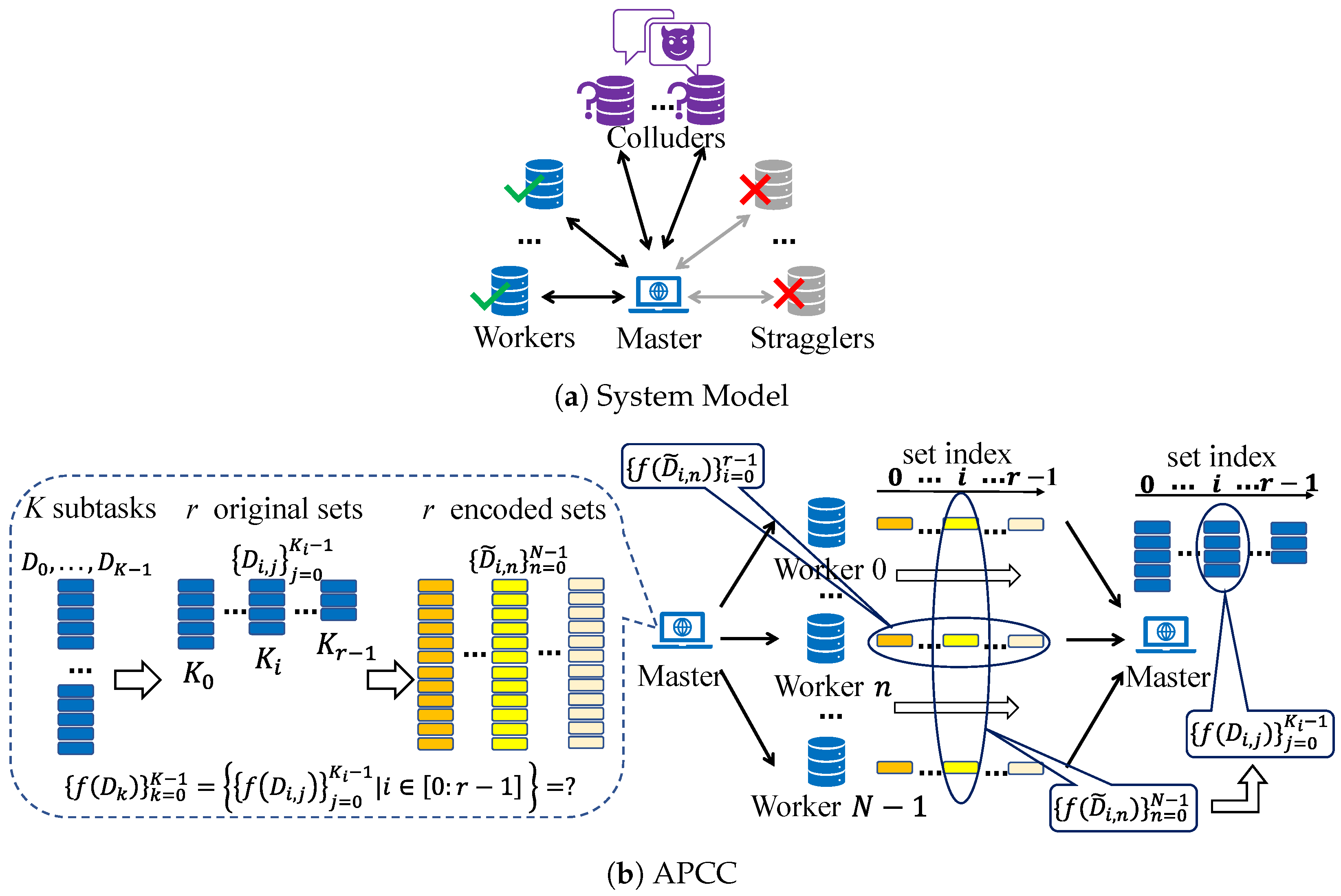
As shown in
Figure 2, we consider the distributed computing system consisting of one master and
N workers. The goal is to complete a computation task on the master with the help of
N workers. The task is represented by a function
f, operating over an equally pre-divided input dataset
. The master aims to evaluate the results
, whose dimensions are decided by the task function
f. To achieve this, we employ the proposed APCC strategy. Note that we consider the computation of
as the entire task and the computation of
as a subtask.
In APCC, the
K equally pre-divided input data
are not directly encoded like conventional coded computing strategies. Instead, they are firstly partitioned into
r sets. Subsequently, the input data in each set are encoded into
N parts, which are then assigned to
N workers for parallel computation. This hierarchical task partitioning structure enables workers to return partial results of assigned subtasks, further mitigating the straggling effect and reducing delays. After the task assignment, the master leverages the results obtained from a subset of workers in each set and employs interpolation methods to reconstruct the original function
f, thereby achieving the recovery of
. A comprehensive description of the APCC strategy is presented in
Section 3.
Taking into account the unreliable channels and uncertain computation capabilities of workers, some of them may fail to return results to the master in time. These straggling workers are referred to as stragglers. Additionally, we assume that workers are honest but curious. This means they will send back the correct computation results, but there could be up to L colluding workers who can communicate with each other and attempt to learn information about the input data . These workers are called colluders.
4. Performance Analysis
In this section, we first define a metric called
encoding rate to evaluate the efficiency performance of coded computing schemes, in terms of utilizing computation resources of workers as efficiently as possible. Then, based on the optimal recovery threshold of LCC [
15], we rigorously prove APCC for accurate results is also an optimal polynomial coding in terms of the encoding rate. Furthermore, an information-theoretic guarantee to completely preserve the privacy of input data
in APCC is proved. Subsequently, we present an analysis of the approximation error for Case 2 of APCC, along with a discussion of numerical stability. At the end of this section, we provide an analysis of encoding and decoding complexity for APCC and compare it with other state-of-the-art strategies.
4.1. Optimality of APCC in Terms of Encoding Rate
To evaluate the performance of various coded computing schemes, a metric known as the encoding rate
is used. This metric is defined as:
where
K is the number of subtasks before encoding,
N is the number of subtasks after encoding (which is equivalent to the number of workers), and
S represents the number of straggling workers that failed to return results before the task was completed. Similar metrics, such as those found in [
17,
20,
46], have also been developed.
Furthermore, since the recovery threshold, denoted by H, is defined as the minimum number of results needed to guarantee decodability, we have and thus . It is important to note that the encoding rate only applies when decodability is guaranteed.
The physical significance of the encoding rate is the ratio between the computation load of tasks before encoding and that required after encoding. For instance, given a task with a computation load of , each subtask has a corresponding load of . As subtasks are successfully completed, the required computation load is . Since coded computing essentially trades computation redundancy for reduced delay to mitigate the straggling effect, it is reasonable to use this metric to evaluate the efficiency of different schemes.
Before demonstrating the optimality of APCC in terms of encoding rate, we present the definitions of capacity and linear coded computing schemes.
Definition 1. A linear coded computing scheme is one in which the encoded data is a linear combination of the original input data as follows:where is the encoding matrix and are additive random real matrices. For example, according to Equation (
2) in APCC,
are the coefficient terms before
, and
represents the sum of added random matrices in
. The index
i corresponds to the set index of the hierarchical task partitioning structure of APCC and can be discarded in other coded computing strategies.
Definition 2. For a coded computing problem , where N is the number of workers, S and L denote the number of stragglers and colluders, respectively, and the computation function f on the master is a polynomial function of degree d, the capacity C is defined as the supremum of the encoding rate as:over all feasible linear coded computing schemes that can address up to L colluders and S stragglers. As illustrated in
Section 3, APCC is a linear coded computing scheme and its hierarchical structure results in different
and
for each set, with
and
representing the number of subtasks before encoding and that of straggling workers, respectively. For set
i,
represents the number of workers that have successfully returned results in time, implying that the number of stragglers is
. Moreover, according to Equation (
11), set
i is considered complete when
. Hence, the encoding rate of APCC can be calculated as:
or the uncoded version for
:
where the equality holds when
N can be divided by
.
The following theorem shows that the encoding rate of APCC achieves the capacity, thereby establishing its optimality. In fact, the optimality of APCC in encoding rate is attributed to its identical polynomial coding structure when compared to LCC [
15], despite having different function expressions. Specifically, for the accurate results case of APCC, the encoding and decoding processes are achieved through Barycentric polynomial interpolation; for LCC, the processes are achieved through Lagrange polynomial interpolation. Although these two formats can be transformed into each other, the Barycentric polynomial format requires less computational complexity and has stronger numerical stability [
27,
44]. For the sake of clarity, we omit the set index
i in APCC and focus on a specific set, without loss of generality.
Theorem 1. For a coded computing problem , where N is the number of workers, S and L denote the number of stragglers and colluders, respectively, and the computation function f on the master is an arbitrary polynomial function of degree d, the capacity C is given by: Proof. To prove Theorem 1, a lower bound on the capacity
C is first established, which follows the encoding rate of APCC in (
20) and (
21). To establish the upper bound, we leverage the optimality statement of LCC, as illustrated in Theorems 1 and 2 of [
15], which shows that polynomial coded computing strategies are able to decode returned computing results successfully only if the following condition is met:
Therefore, we have:
Equation (
24) presents the maximum number of task divisions permissible to ensure decodability, given the numbers of workers
N, stragglers
S, and colluders
L. The reason is that the more divisions there are, the more results are needed from workers. However, there are at most
N workers, including
S stragglers, to return results. Based on (
24), an upper bound on the encoding rate can be derived as:
Since the capacity
C is the supremum of
, it also has the same upper bound. With the lower bound provided previously, we can conclude that APCC is an optimal coded computing strategy that can reach the capacity in (
22). □
To enhance clarity, the fundamental proof for the derivation of (
23) is briefly introduced in
Appendix A, following the same steps as outlined in [
15].
Please note that the conclusion presented in this subsection pertains only to accurately coded computing. For approximated coded computing, the use of different approximation methods can lead to varying errors, making it challenging to compare and analyze their impact on the encoding rate and capacity in a qualitative manner.
4.2. Guarantee of the Privacy Preservation
Recall that colluders are those workers who can communicate with each other and attempt to learn something about the original input data. Since the system can tolerate at most L colluders, we assume that there are colluders, where and the user does not know which workers are colluding. We use the index set to denote the colluding workers, where .
Assuming that the input data
are independent of each other, we denote the encoded input data sent to workers in the colluding set
for set
i as:
Therefore, the information-theoretic privacy-preserving constraint can be expressed as:
where
represents the mutual information function.
With the assumption of finite precision floating point arithmetic, the values of elements in the data matrices such as
,
, and
come from a sufficiently large finite field
. Assuming that the size of these data matrices is
, we have
where
is due to the fact that all random matrices
are independent of the input data
.
is because the entropy of each element in the random matrices equals
, and
follows from the upper bound of the entropy of each element in
being
. Since the mutual information is non-negative, it must be 0, which guarantees complete privacy preservation.
Note that the analysis in this subsection is applicable to both accurate and approximated cases. This is because the analysis only involves the encoding and assignment steps of APCC, and both cases require the same two initial steps. The key difference between the two aforementioned cases is reflected in the decoding functions with distinct adaptive parameters , which correspond to Barycentric polynomial interpolation and Berrut’s rational interpolation, respectively.
4.3. Analysis of Approximation Error for Case 2
According to the discussion in [
27], the approximation error of Berrut’s rational polynomial interpolation used for Case 2 in APCC is provided as the following theorem:
Theorem 2 ([
27])
. Let the interpolating objective function have a continuous second derivative on , and the number of received results , the approximation error is upper bounded as:if is even, andif is odd, where . Consequently, for set i and a fixed total number of workers N, the approximation using becomes more accurate as the number of received results increases.
4.4. Numerical Stability
In coded computing, the issue of numerical stability typically arises from the decoding part, which is based on solving a system of linear equations involving a Vandermonde matrix. As previously discussed, Cases 1 and 2 of APCC employ Barycentric polynomial interpolation and Berrut’s rational interpolation as decoding methods, respectively. For Case 1, Barycentric polynomial interpolation demonstrates good performance in addressing errors caused by floating-point arithmetic [
44]. Regarding Case 2, it has been shown in [
27] that the Lebesgue Constant of Berrut’s rational interpolation grows logarithmically with the number of received results from workers, rendering it both forward and backward stable.
4.5. Encoding and Decoding Complexity
In this subsection, we provide the analysis of encoding and decoding complexity. Intuitively, APCC utilizes the hierarchical task partitioning structure to enhance delay performance. However, it does so at the cost of requiring multiple encoding and decoding operations, specifically
r times for the
r sets, when compared to LCC [
15] and BACC [
27].
In LCC and BACC, the encoding operations take N times, corresponding to the number of workers, while the decoding operations take times, equivalent to the number of task divisions. On the other hand, in the case of APCC, which features r partitioned sets, the encoding and decoding operations entail and , respectively. When the computation loads per worker in all strategies are equal, i.e., , it can be deduced that the encoding and decoding operations in APCC are r times those of LCC and BACC.
5. Hierarchical Task Partitioning
In this section, the hierarchical task partitioning is formulated as an optimization problem with the objective of minimizing the task completion delay. The problem is divided into two cases for consideration: with and without cancellation. Through derivations, two mixed integer non-linear programming problems are obtained, and we propose a maximum value descent (MVD) algorithm to obtain the optimal solutions with low computational complexity. Moreover, after analysis, it is found that the MVD algorithm can be quickly executed by selecting the appropriate input. Detailed explanations are provided as follows.
5.1. Problem Formulation
In the context of negligible encoding and decoding delays, with the computation delays of workers being the dominant component, the delay for a worker to complete a single subtask, denoted as
T can be represented by a shifted exponential distribution [
4,
7,
11,
12,
40,
41], whose cumulative distribution function (CDF) is given by:
where
is a parameter indicating the minimum processing time and
is a parameter modeling the computing performance of workers. All
N workers follow a uniform computation delay distribution defined in (
31).
Recall that in the hierarchical structure, the completion of a particular set is dependent on the successful receiving of a sufficient number of results from its encoded subtasks. The overall completion of the entire task is achieved only when all r sets have been completed. Notably, is defined as the threshold number of successful results needed to ensure the completion of set i.
Following the discussion in
Section 3 and assuming that privacy preservation is required which means
, the threshold for
Case 1 of APCC can be expressed as
according to (
11). For
Case 2 of APCC, the threshold
can be determined based on the desired approximation precision, with higher values of
leading to more accurate approximations.
The completion time of sets is defined as
, where
denotes the time interval from the initial moment 0 of the entire task to the recovery moment of set
i. The entire task is considered completed when all
r sets have been recovered. Therefore, we denote the entire task completion delay as
Note that while each worker executes the assigned subtasks in the order of set indices, the order in which these sets are recovered may not be the same. The completion time of sets is influenced not only by the set indices but also by the recovery thresholds
determined by
.
Due to the randomness of delay, our objective is to minimize the entire task completion delay
, upon which the probability of the master recovering desired results for all sets is higher than a given threshold
, as expressed by the following inequality:
where
is defined as the number of returned results for set
i until time
t.
However, to derive (
33), we first need to obtain the distribution of the delay required to receive the last non-straggling result in each set and then derive their joint probability distribution, which is intractable, especially when considering the cancellation of completed sets. As a result, the problem with the constraint (
33) is hard to solve.
In the following, we consider substituting (
33) with an expectation constraint (34d) and formulate the problem as:
where
is the partitioning scheme.
Constraint (
34a) corresponds to the hierarchical task partitioning, and (34c) indicates that the threshold for each set should be smaller than the number of workers. In constraint (34e),
represents the set of positive integers. Constraint (34d) states that the master is expected to receive sufficient results of encoded subtasks from workers to recover
in set
i. Similar approximation approaches are also used in [
4,
12,
40,
41], and the performance gap can be bounded [
12].
As previously shown,
for
Case 1 of APCC. Additionally, the maximum of
for all sets can be replaced with an optimization variable
z by adding an extra constraint. Consequently, for Case 1 of APCC,
can be equivalently written as:
For Case 2 of APCC, one only needs to adjust constraints (35c) and (35d) according to the relationship between and , which does not affect the subsequent methods employed. Consequently, for the sake of convenience in expression, we will focus on Case 1 of APCC in the following parts of this section, without loss of generality.
5.2. APCC without Cancellation
If the cancellation of completed sets is not considered, we first denote the delay of one worker to continuously complete
m subtasks as
, and derive its CDF from (
31) as:
Since computations on workers are independent,
can be written as:
where
denotes the indicator function that equals 1 if event
x is true and equals 0 otherwise.
is given by (
36).
Substituting (
37) into
, we find (35d) is covered by (35c) and obtain the following optimization problem:
As
shows, it is a mixed integer non-linear programming (MINLP) problem, which is usually NP-hard. Although its optimal solution can be found by the Branch and Bound (B&B) algorithm [
47], the computational complexity is up to
, which means the B&B algorithm becomes extremely time-consuming when either
N or
r are large.
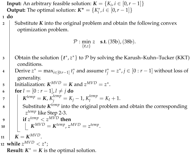
Accordingly, to efficiently obtain an optimal solution, we propose the maximum value descent (MVD) algorithm shown in Algorithm 2. The key idea of the MVD algorithm is to iteratively update the input solution by adjusting for the set that corresponds to the maximum value descent of the objective function z. In the MVD algorithm, each do-while loop can be regarded as one update, and in Step 7 constantly approaches the optimal . Once reduced in an update, will not increase because the objective function z must decrease in each update. When the updating process terminates, the optimal solution is exactly the obtained in the last update. Furthermore, the MVD algorithm has a computational complexity of , as the number of do-while loops is determined by constraint (35d).
Furthermore, the MVD algorithm can be executed quickly by selecting a sufficiently good partitioning solution as input. It should be noted that after relaxation and cancellation of the integer constraint in (35e),
can be transformed into a convex problem as follows:
and the optimal solution is given in Proposition 1 according to the Karush–Kuhn–Tucker (KKT) conditions.
| Algorithm 2: MVD |
![Entropy 26 00881 i002]() |
Proposition 1. For given , the optimal solution and corresponding delay to are Due to the convexity of , the Euclidean distance between and the optimal solution of is small. Therefore, it is recommended to use a rounded result of as the input for the MVD algorithm.
5.3. APCC with Cancellation
If the cancellation of completed sets is considered, a worker may be canceled in a certain set but successfully return results in time for the subsequent sets. For example, worker
n may be a straggler for set
i but completes its assigned subtask and returns the result in time for the next set
due to the cancellation. Such situations make it quite difficult to derive and analyze the expectation of
as in the previous
Section 5.2, because the impact of the cancellation of the previous set on the delay of non-straggling workers in subsequent sets needs to be considered. Therefore, we provide the following alternative perspective to simplify this problem.
Note that if set
i is the last completed one, the entire task is completed when the last needed result for this set is received. Thus, we define the delay of set
i as
and aim to minimize
. To derive
, consider that there are still
workers computing the last result for set
i when other sets are finished. Once any one of these workers returns the first result, this set and the entire task will be completed. Accordingly, the CDF of
can be written as follows:
where
is the delay needed to complete
subtasks for one worker, shown previously in (
36). Then we have
By further adding an extra optimization variable
z to substitute
, the optimization problem can be formulated as:
Note that
is a MINLP problem similar to
and has an
computational complexity to solve if using B&B algorithm. However, after relaxation and canceling the integer constraint in (35e),
can also be transformed into a convex problem as:
and optimal solution is given in Proposition 2 according to the KKT conditions.
Proposition 2. For given , the closed-form expression of the optimal solution to is Consequently, the MVD algorithm is used again to solve with a computational complexity of , and the rounded result of is recommended to be used as the input.
6. Simulation Results
In this section, we leverage simulation results to evaluate the performance of APCC in terms of task completion delay and compare it with other state-of-the-art coded computing strategies, including LCC [
15], LCC with multi-message communications (LCC-MMC) [
35], and BACC [
27]. Additionally, we analyze the impact of the number of partitioned sets
r and the number of colluding workers
L on the task completion delay of APCC.
In simulations, the entire task is given, leading to a constant computation load for the entire task. In this scenario, we aim to compare the entire task completion delay across various task divisions and coded computing strategies, illustrating the delay performance improvements introduced by APCC. We assume that the computation delay
of a single worker to complete the entire task follows a shifted exponential distribution, which is modeled as:
then the computation delay
T of a single worker to complete one subtask follows:
where
K denotes the task division number, which may vary depending on the chosen coded computing strategies. The parameter
is set to
s, and
is set as
. In APCC,
corresponds to the number of subtasks in each set before encoding, and their values are obtained using the MVD algorithm. Then,
Monte Carlo realizations are run to obtain the average completion delay of the entire task, and the simulation codes are shared here (code link:
https://github.com/Zemiser/APCC, accessed on 24 August 2024). Note that by comparing (
47) with (
31), we have
and
, and can further derive the distribution of
in (
36).
The benchmarks involved in this section are as follows:
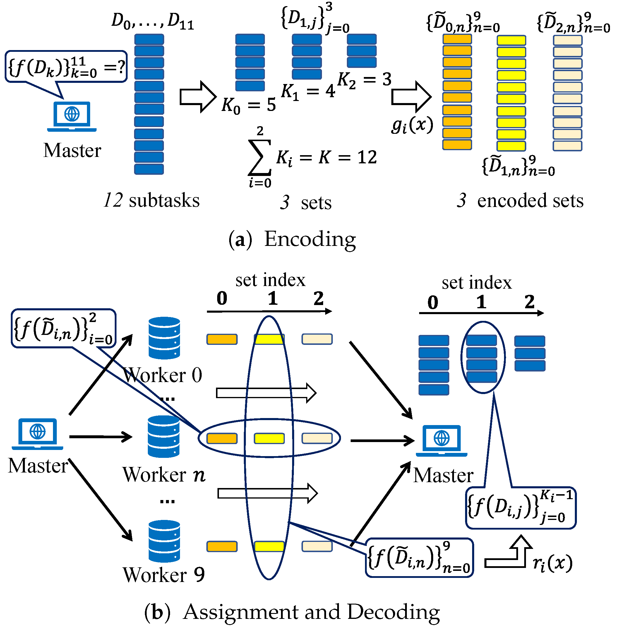
(1) APCC: APCC is our proposed coded computing strategy in this paper. It first divides the entire task into K subtasks and then partitions them into r sets with different sizes. The number of subtasks in set is denoted as , which satisfies . After that, each set is encoded into N subtasks assigned to the N workers. Consequently, each worker is assigned r subtasks. For Case 1 of APCC, the set i is recovered when the master has received results, and the entire task is completed when all sets are recovered.
(2) LCC: LCC proposed in [
15] divides the entire task into
subtasks and then encodes them into
N subtasks assigned to
N workers. Each worker in LCC is assigned one subtask. Therefore, the entire task is completed when the master has received
results.
means the absence of a requirement for privacy preservation. We assume that the number of workers
N is greater than
to facilitate our analysis. Consequently, when
, the recovery threshold is defined as
instead of
according to [
15].
(3) LCC-MMC: MMC proposed in [
35] is another approach to utilize the computing results of straggling workers except for the hierarchical structure. It also achieves a partial return of results from workers through a more granular task division. Specifically, LCC-MMC divides the entire task into
subtasks and then encodes them into
subtasks. Each worker in LCC-MMC is assigned
r subtasks and the entire task is completed when the master has received
results. However, LCC-MMC cannot preserve the privacy of input data because multiple encoded data from the same encoding function are sent to a worker, which is different from the case of APCC where
r subtasks assigned to the same worker are generated by
r different encoding functions
.
(4) BACC: The BACC strategy, as introduced in [
27], offers approximated results with improved precision achievable by increasing the number of return results from workers. It shares a task division structure identical to LCC, partitioning the task into
subtasks and then further encoding them into
N subtasks. Each worker in BACC is assigned one such subtask.
To ensure fairness, all strategies employ an identical number of workers and distribute an equivalent computation load for a single worker. Assuming that the computation loads of the entire task are
, then each subtask
in APCC has a computation load of
, and the computation loads of each worker in APCC are
because there are
r partitioned sets. Similarly, we can derive that the computation loads of each worker in LCC, BACC and LCC-MMC are
,
and
, respectively. In order to ensure that each worker in these schemes performs an identical fraction of the entire task as APCC, we have
Due to the different applicability of various coded computing strategies, we will first conduct a comprehensive analysis and comparison of APCC alongside other strategies within the following three scenarios: (1) Accurate results with L colluding workers (); (2) Accurate results without colluding workers (); (3) Approximated results. Finally, we study the impact of the parameters r and L on the delay performance of APCC.
6.1. Accurate Results with L Colluding Workers ()
In this scenario, we consider the following three benchmarks: LCC, APCC without cancellation, and APCC with cancellation. For fair comparison, the computation load of workers should be set the same, so we have .
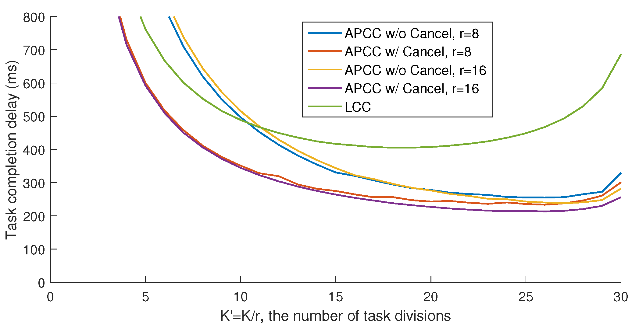
As shown in
Figure 5, the average completion delay of the entire task
first decreases and then increases with the task division number
K, indicating the existence of an optimal division that minimizes the delay. This trade-off arises from balancing the computation load of each worker and the minimum number of workers needed to recover
. On the one hand, as the division number decreases, the computation load of each subtask increases, which leads to longer computation delays for each worker due to the increased workload. Although the number of workers waiting for results decreases, the increase in load negates this advantage. On the other hand, while the division number approaches the maximum, as illustrated in the inequality (
24), the number of workers that the master needs to wait for approaches
N, making the straggling effect a bottleneck for performance and increasing the delay. The zigzag fluctuations in the curve are mainly due to the integer values of the partitioning numbers.
Note that the primary metric for evaluating different schemes in our study is the minimum task completion delay under different division numbers, as depicted in
Figure 5. This is because the division number
corresponds to the division of computation function inputs, which is typically a high-dimensional matrix. As such,
can be adjusted flexibly in most cases. Therefore, the minimum achieved task completion delay is the main focus of our analysis.
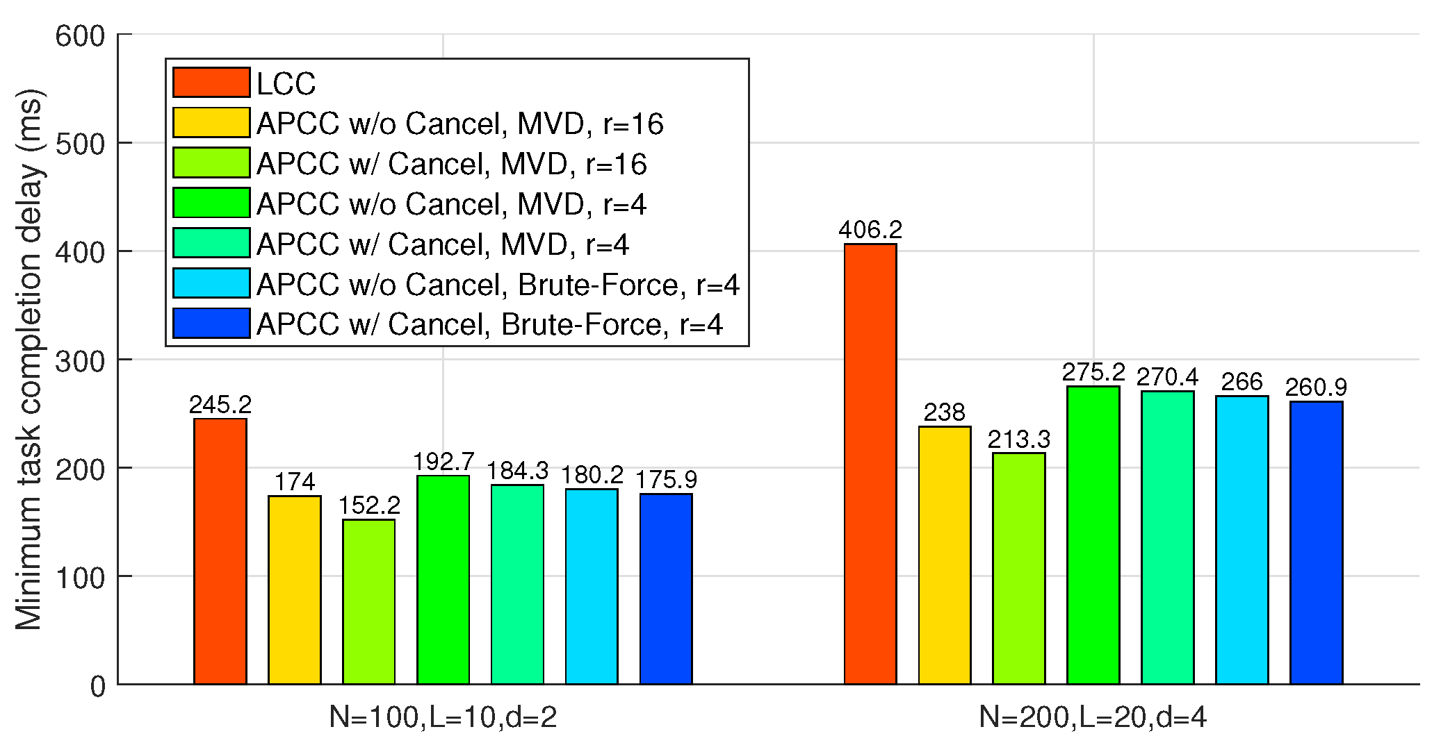
Figure 6 compares APCC and LCC in terms of the minimum task completion delay. In these benchmarks, ‘Brute-Force’ refers to a partitioning strategy derived from an exhaustive search across all possible values of
. Due to the highly complex traversal search, the brute-force results are only provided for scenarios with a smaller number of sets (
).
Figure 6 illustrates that both APCC with and without cancellation yield sufficient reductions in task completion delay compared to LCC. For instance, when
,
,
,
, and the partitioning strategy obtained from the MVD algorithm is utilized, APCC with and without cancellation achieve delay reductions of
and
, respectively, compared to LCC. Moreover, the comparison with the ‘Brute-Force’ benchmarks shows that the partitioning strategy
obtained through the MVD algorithm is near-optimal.
6.2. Accurate Results without Colluding Workers ()
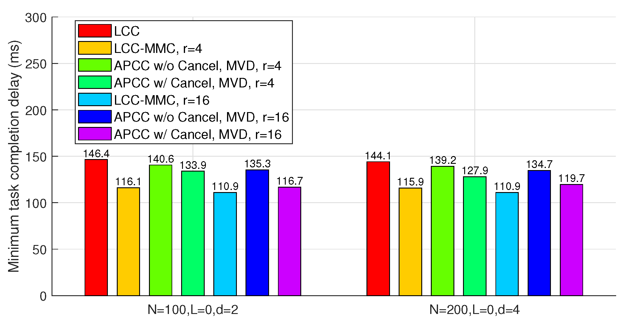
In this scenario, we evaluate four benchmarks: LCC, LCC-MMC, and APCC with and without cancellation. Among these, only LCC does not consider partial results from straggling workers. Similar to Subsection IV.A, we set , with representing the task division number for LCC-MMC.
In
Figure 7, both LCC-MMC and APCC effectively reduce task completion delay compared to LCC. Specifically, when
r is large enough, APCC with cancellation closely approaches the performance of LCC-MMC. This similarity arises because, in both APCC and LCC-MMC, the master utilizes nearly all computing results from workers when divided subtasks are sufficiently small.
Figure 7 also illustrates that when privacy is not a concern, MMC is a viable method to reduce the delay in coded computing.
Compared to
Figure 6, we observe that the absence of colluding workers limits the potential for delay optimization. For instance, with parameters
,
,
, and
, APCC with cancellation achieves only a
delay reduction compared to LCC.
6.3. Approximated Results
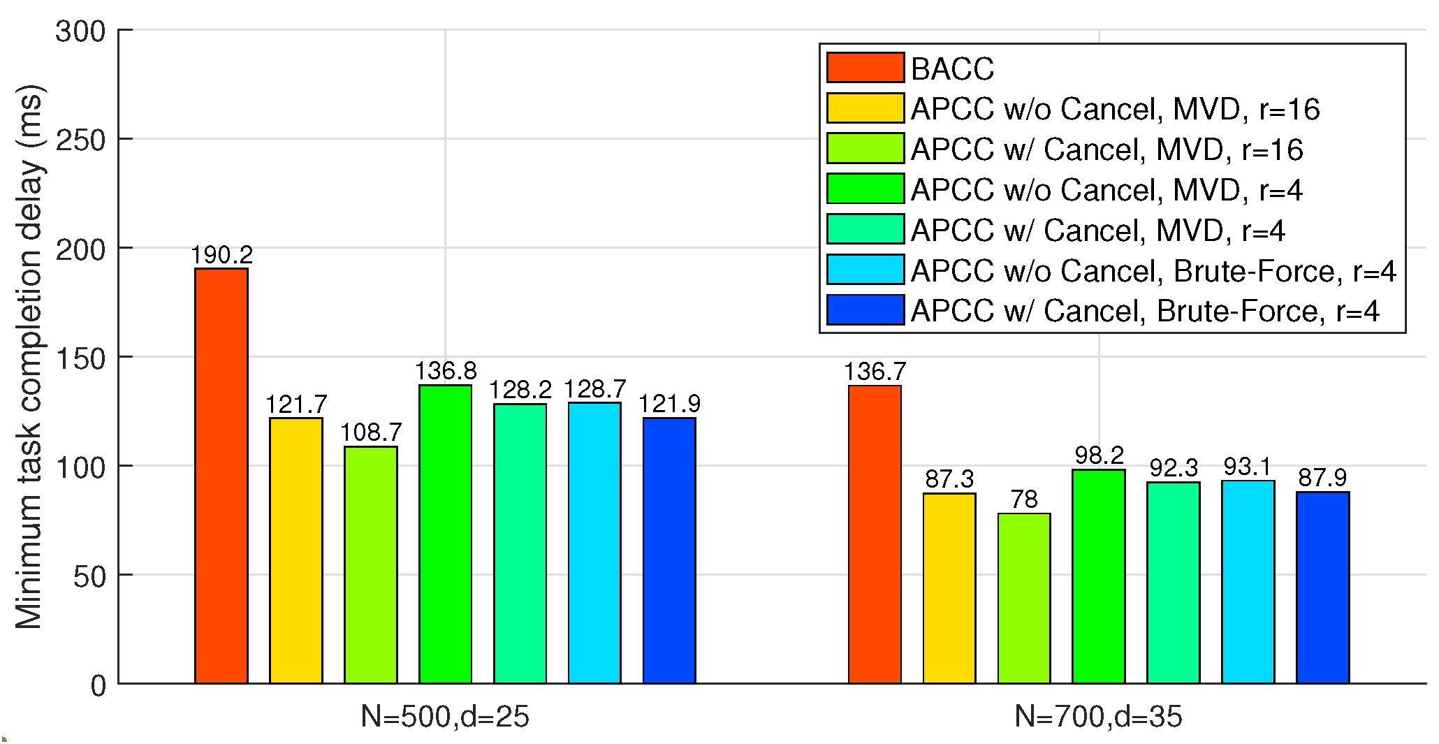
In this subsection, we compare the task completion delay of BACC and case 2 of APCC, which can both provide approximated results with fewer workers than the recovery threshold. To ensure uniform worker computation load, we also set , as in our previous analysis. Furthermore, since BACC shares an identical task division structure with LCC, we employ a smaller recovery threshold of the same form as LCC to evaluate its delay performance. For instance, when the recovery threshold exceeds N, a reduced uniform recovery threshold below N can be employed for both BACC and APCC.
As shown in
Figure 8, the hierarchical task partitioning and the cancellation of completed sets in APCC yield sufficient delay performance improvement. Compared to BACC, the proposed MVD algorithm for APCC achieves up to
delay reduction. Note that in this scenario, both APCC and BACC can obtain approximated results with fewer returned results, while LCC for accurate computation fails to work when
is larger than 20 in the two cases of
Figure 8, as the recovery threshold of LCC needs to be larger than
.
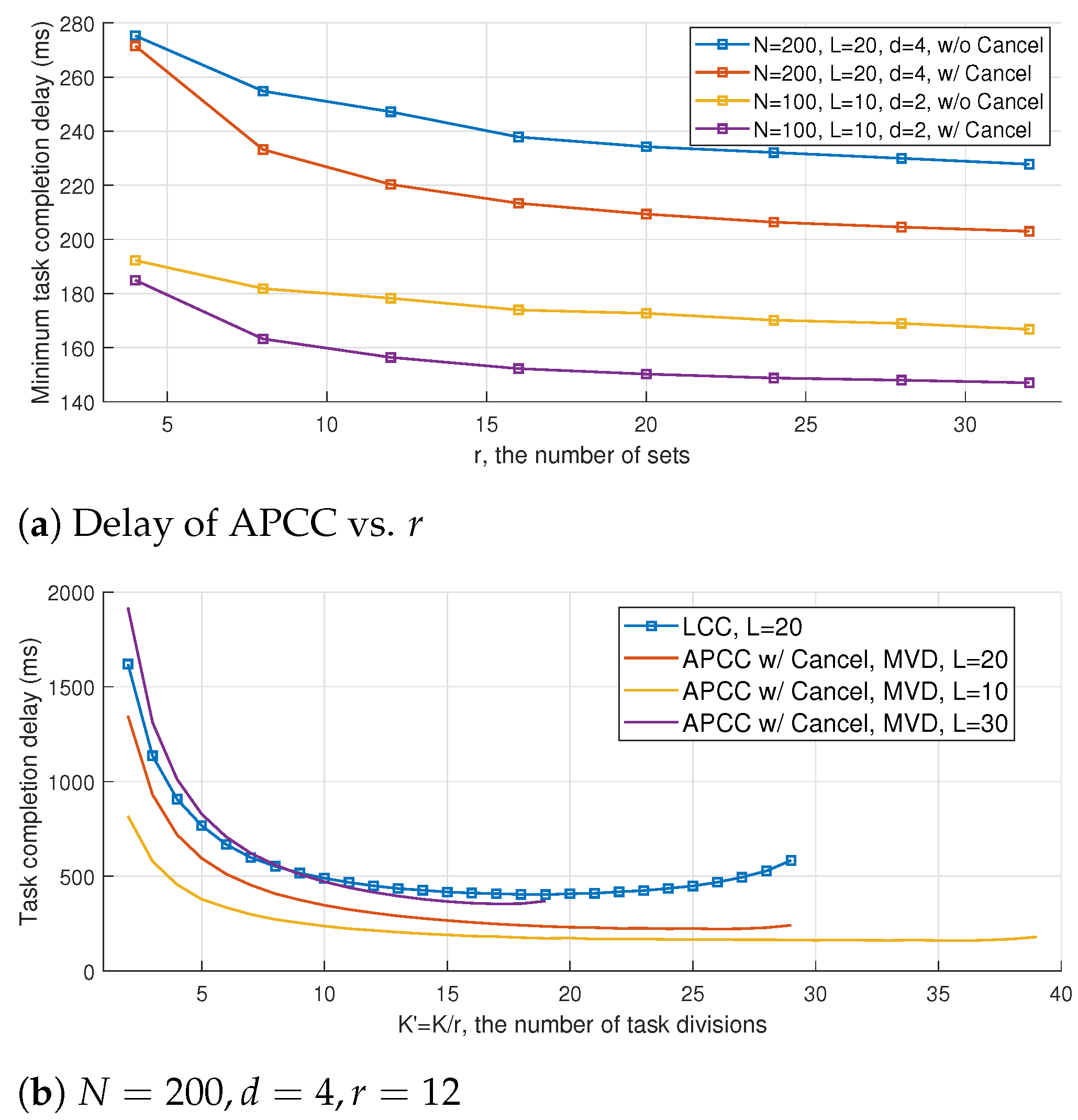
6.4. Impact of r and L on the Performance of APCC
The impact of the hierarchical partitioning number of sets
r on the task completion delay of APCC is illustrated in
Figure 9a. It is observed that a larger number of sets
r results in a smaller computation delay, which is consistent with the results shown in previous figures. The reduction in delay can be attributed to the fact that a larger
r implies a smaller computation load for each subtask in the hierarchical structure, and the difference in computation load between fast and slow workers can be described more precisely. Consequently, the proposed MVD algorithm can better utilize the computing results of straggling workers to reduce delay. Furthermore,
Figure 9a indicates that the benefit of increasing
r has a boundary effect, which corresponds to the upper bound of benefit brought by the granularity refinement of task divisions.
Recall that
L denotes the maximum number of colluding workers that a coded computing scheme can tolerate. The value of
L can serve as an indirect indicator of the level of privacy preservation offered by the scheme. Specifically, a larger value of
L corresponds to more stringent privacy protection and a higher tolerance for colluders. It is demonstrated in
Section 4.2 that complete data privacy can be achieved as long as the number of colluders remains below
L.
Figure 9b illustrates the impact of the number of colluding workers
L on the trade-off between delay and privacy preservation. It is worth noting that, for a fixed
, increasing the value of
L leads to a larger recovery threshold
H for the original subtasks, which results in a longer task completion delay. Moreover, as demonstrated in (
24), choosing a larger value of
L restricts the maximum number of task divisions. Consequently, the range of
values corresponding to the plotted curves in
Figure 9b varies with
L.


