

Engineering Transport via Collisional Noise: A Toolbox for Biology Systems


Abstract
:1. Introduction
2. Model and Numerical Method
3. Results
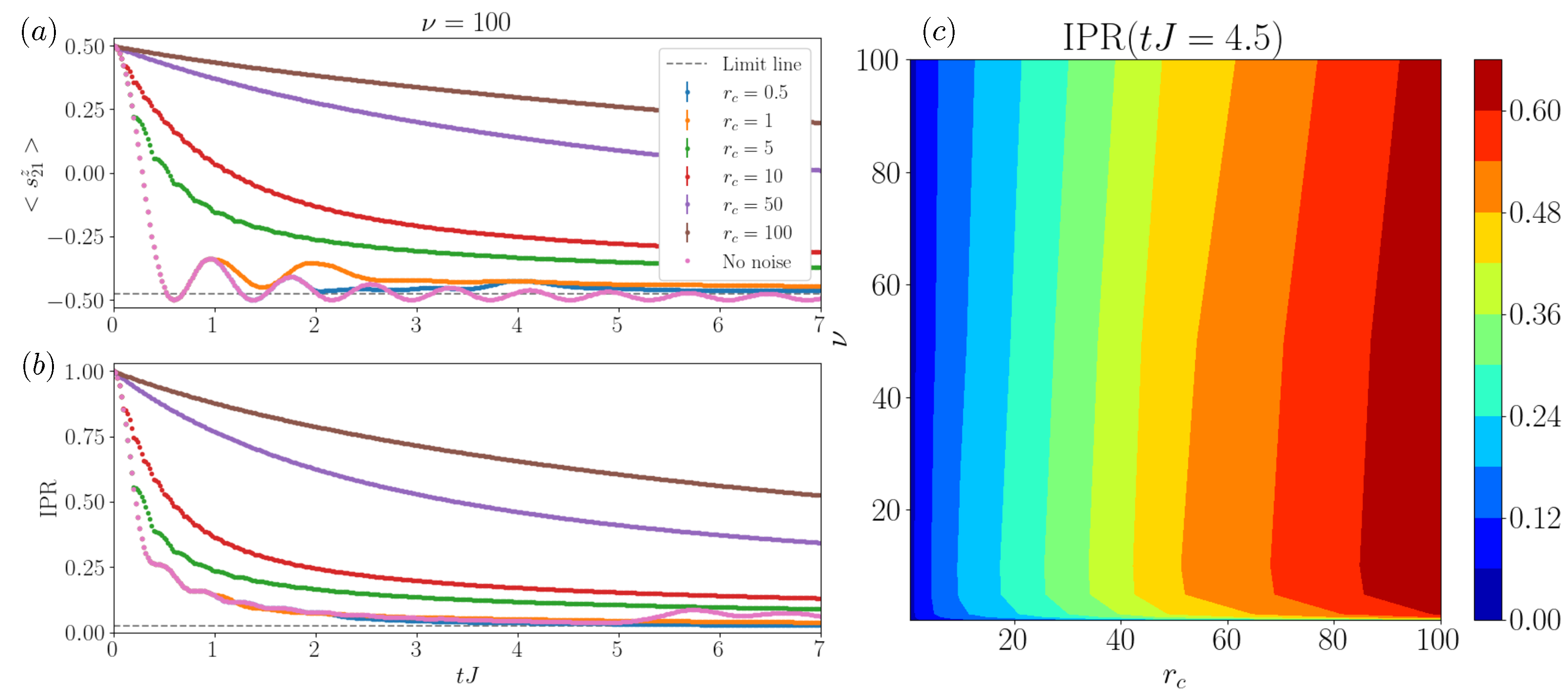
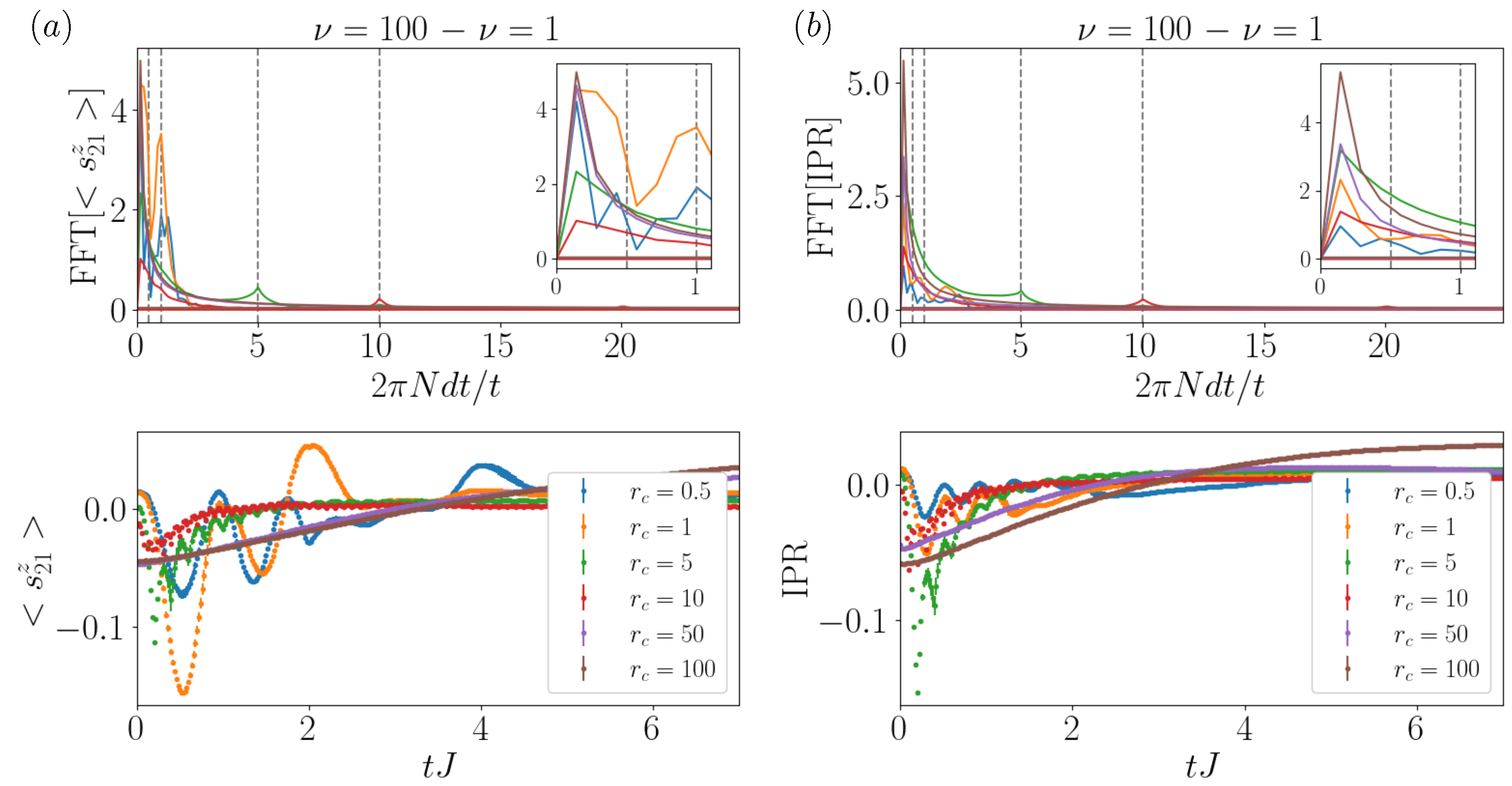
3.1. One Excitation
3.2. Multiple Excitations
4. Discussion
Author Contributions
Funding
Data Availability Statement
Acknowledgments
Conflicts of Interest
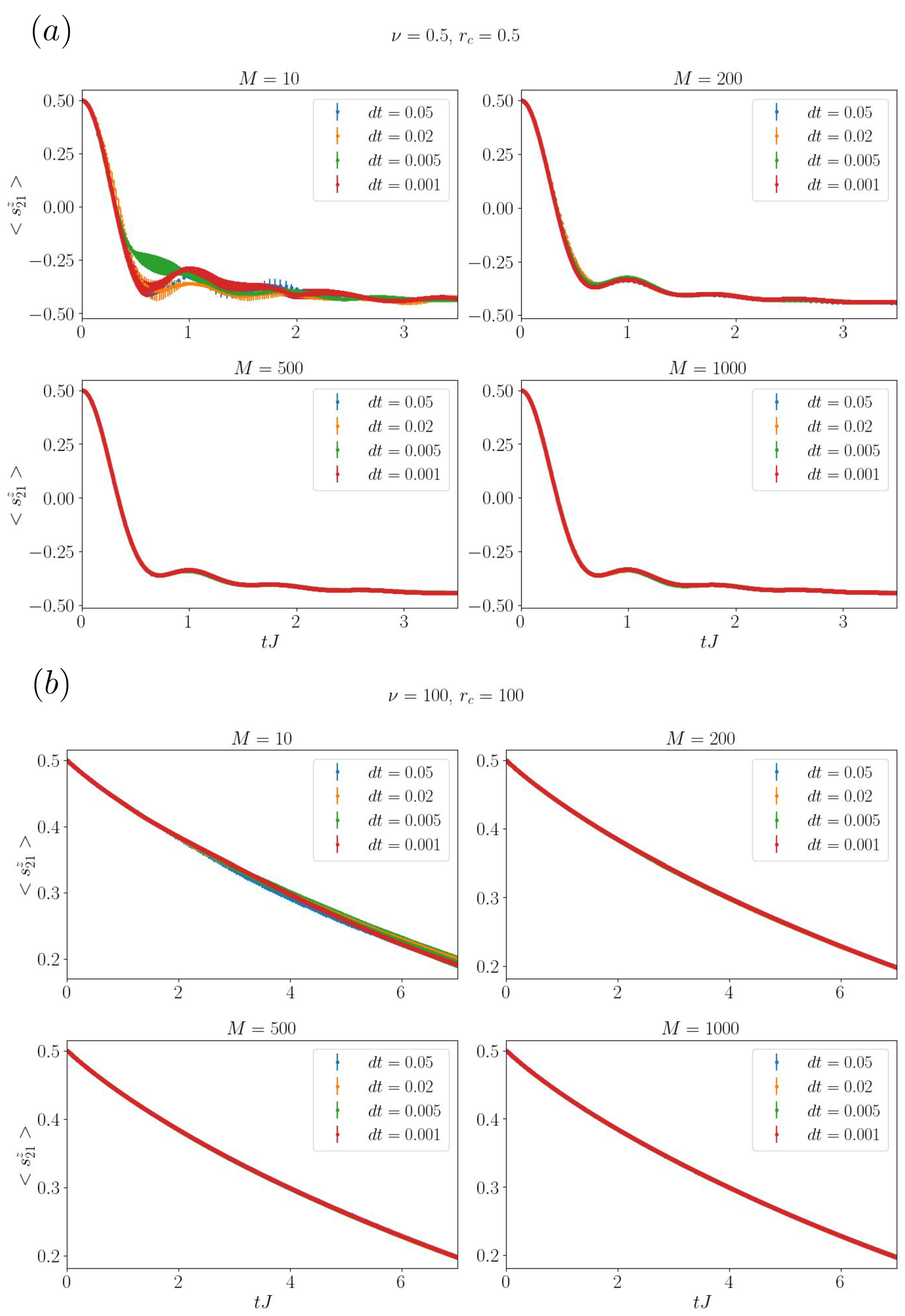
Appendix A. Convergence Analysis

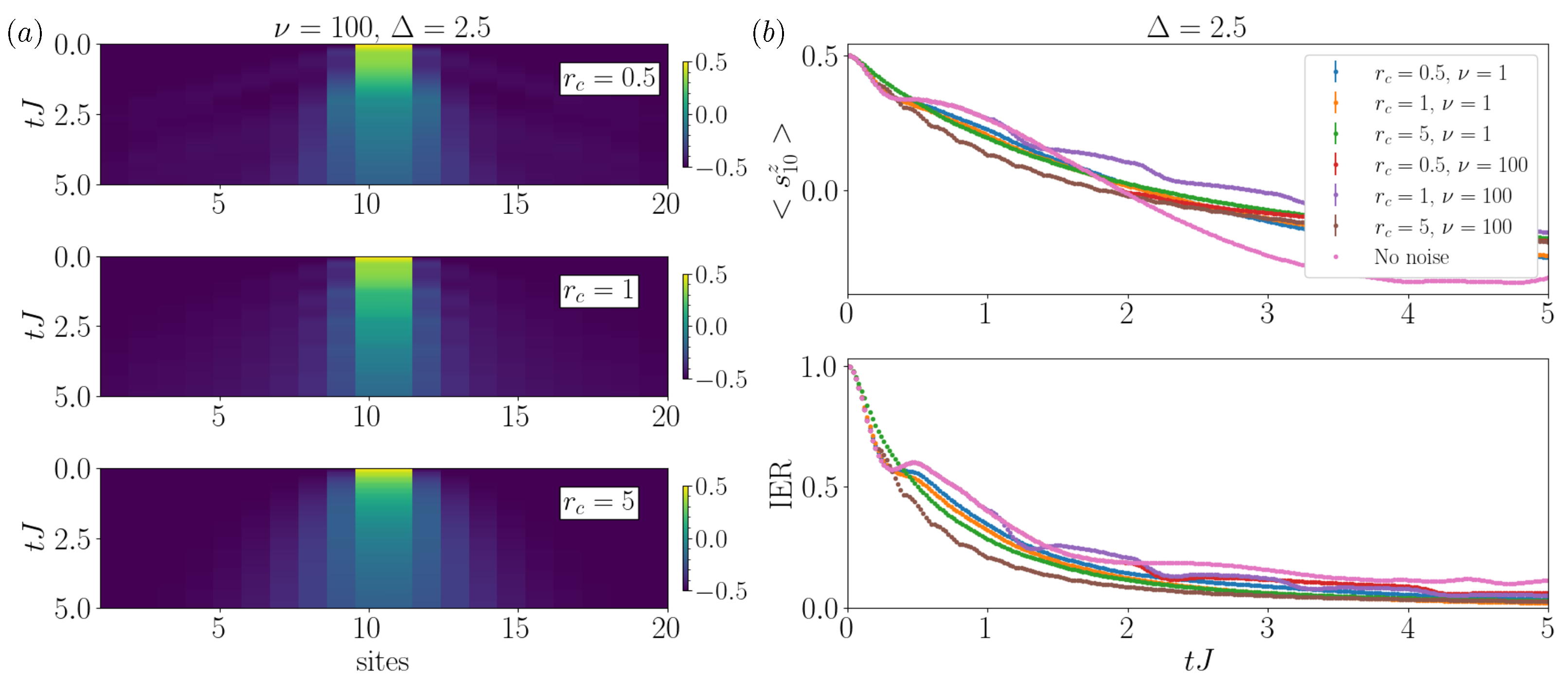
Appendix B. Case Δ = 2.5
References
- Wiseman, H.; Milburn, G. Quantum Measurement and Control, 2nd ed.; Cambridge University Press: Cambridge, UK, 2010; pp. 148–215. [Google Scholar]
- Breuer, H.; Petruccione, F. The Theory of Open Quantum Systems, 2nd ed.; Oxford University Press: Oxford, UK, 2002; pp. 390–498. [Google Scholar]
- Gardiner, C.; Zoller, P. Quantum Noise, 1st ed.; Springer: Berlin/Heidelberg, Germany, 2005; pp. 212–243. [Google Scholar]
- Daley, A. Quantum trajectories and open many-body quantum systems. Adv. Phys. 2014, 63, 77–149. [Google Scholar] [CrossRef]
- Harrington, P.M.; Mueller, E.J.; Murch, K.W. Engineered dissipation for quantum information science. Nat. Rev. Phys. 2022, 4, 660–671. [Google Scholar] [CrossRef]
- Diehl, S.; Tomadin, A.; Micheli, A.; Fazio, R.; Zoller, P. Dynamical Phase Transitions and Instabilities in Open Atomic Many-Body Systems. Phys. Rev. Lett. 2010, 105, 015702. [Google Scholar] [CrossRef] [PubMed]
- Kessler, E.M.; Giedke, G.; Imamoglu, A.; Yelin, S.F.; Lukin, M.D.; Cirac, J.I. Dissipative phase transition in a central spin system. Phys. Rev. A 2012, 86, 012116. [Google Scholar] [CrossRef]
- Vicentini, F.; Minganti, F.; Rota, R.; Orso, G.; Ciuti, C. Critical slowing down in driven-dissipative Bose-Hubbard lattices. Phys. Rev. A 2018, 97, 013853. [Google Scholar] [CrossRef]
- Li, Y.; Chen, X.; Fisher, M.P.A. Quantum Zeno effect and the many-body entanglement transition. Phys. Rev. B 2018, 98, 205136. [Google Scholar] [CrossRef]
- Skinner, B.; Ruhman, J.; Nahum, A. Measurement-Induced Phase Transitions in the Dynamics of Entanglement. Phys. Rev. X 2019, 9, 031009. [Google Scholar] [CrossRef]
- Li, Y.; Chen, X.; Fisher, M.P.A. Measurement-driven entanglement transition in hybrid quantum circuits. Phys. Rev. B 2019, 100, 134306. [Google Scholar] [CrossRef]
- Bao, Y.; Choi, S.; Altman, E. Theory of the phase transition in random unitary circuits with measurements. Phys. Rev. B 2020, 101, 104301. [Google Scholar] [CrossRef]
- Cao, X.; Tilloy, A.; Luca, A.D. Entanglement in a Free Fermion Chain under Continuous Monitoring. ScyPost Phys. 2019, 7, 024. [Google Scholar] [CrossRef]
- Müller, T.; Diehl, S.; Buchhold, M. Measurement-Induced Dark State Phase Transitions in Long-Ranged Fermion Systems. Phys. Rev. Lett. 2022, 128, 010605. [Google Scholar] [CrossRef] [PubMed]
- Panitchayangkoon, G.; Hayes, D.; Fransted, K.A.; Caram, J.R.; Harel, E.; Wen, J.; Blankenship, R.E.; Engel, G.S. Long-lived quantum coherence in photosynthetic complexes at physiological temperature. Proc. Natl. Acad. Sci. USA 2010, 107, 12766–12770. [Google Scholar] [CrossRef] [PubMed]
- Fleming, G.R.; Scholes, G.D.; Cheng, Y.C. Quantum effects in biology. Procedia Chem. 2011, 3, 38–57. [Google Scholar] [CrossRef]
- Cao, J.; Cogdell, R.J.; Coker, D.F.; Duan, H.G.; Hauer, J.; Kleinekathöfer, U.; Jansen, T.L.C.; Mančal, T.; Miller, R.J.D.; Ogilvie, J.P.; et al. Quantum biology revisited. Sci. Adv. 2020, 6, eaaz4888. [Google Scholar] [CrossRef] [PubMed]
- Collini, E.; Wong, C.Y.; Wilk, K.E.; Curmi, P.M.G.; Brumer, P.; Scholes, G.D. Coherently wired light-harvesting in photosynthetic marine algae at ambient temperature. Nature 2010, 463, 644–647. [Google Scholar] [CrossRef] [PubMed]
- Huelga, S.; Plenio, M. Vibrations, quanta and biology. Contemp. Phys. 2013, 54, 181–207. [Google Scholar] [CrossRef]
- Olaya-Castro, A.; Lee, C.F.; Olsen, F.F.; Johnson, N.F. Efficiency of energy transfer in a light-harvesting system under quantum coherence. Phys. Rev. B 2008, 78, 085115. [Google Scholar] [CrossRef]
- Plenio, M.B.; Huelga, S.F. Dephasing-assisted transport: Quantum networks and biomolecules. New J. Phys. 2008, 10, 113019. [Google Scholar] [CrossRef]
- Ziman, M.; Stelmachovic, P.; Buzek, V. Description of quantum dynamics of open systems based on collision-like models. Open Syst. Inf. Dyn. 2005, 12, 81–91. [Google Scholar] [CrossRef]
- Ciccarello, F.; Palma, G.; Giovannetti, V. Collision-model-based approach to non-Markovian quantum dynamics. Phys. Rev. 2013, 87, 040103. [Google Scholar] [CrossRef]
- Vacchini, B. General structure of quantum collisional models. Int. J. Quantum Inf. 2014, 12, 1461011. [Google Scholar] [CrossRef]
- Lorenzo, S.; Ciccarello, F.; Palma, G. Composite quantum collision models. Phys. Rev. 2017, 96, 032107. [Google Scholar] [CrossRef]
- Ciccarello, F. Collision models in quantum optics. Quantum Meas. Quantum Metrol. 2017, 4, 53–63. [Google Scholar] [CrossRef]
- Cilluffo, D.; Carollo, A.; Lorenzo, S.; Gross, J.; Palma, G.; Ciccarello, F. Collisional picture of quantum optics with giant emitters. Phys. Rev. Res. 2020, 2, 043070. [Google Scholar] [CrossRef]
- Seah, S.; Nimmrichter, S.; Grimmer, D.; Santos, J.; Scarani, V.; Landi, G. Collisional quantum thermometry. Phys. Rev. Lett. 2019, 123, 180602. [Google Scholar] [CrossRef] [PubMed]
- Guarnieri, G.; Morrone, D.; Cakmak, B.; Plastina, F.; Campbell, S. Non-equilibrium steady-states of memoryless quantum collision models. Phys. Lett. 2020, 384, 126576. [Google Scholar] [CrossRef]
- Campbell, S.; Vacchini, B. Collision models in open system dynamics: A versatile tool for deeper insights? Europhys. Lett. 2021, 133, 60001. [Google Scholar] [CrossRef]
- Cattaneo, M.; Chiara, G.D.; Maniscalco, S.; Zambrini, R.; Giorgi, G. Collision models can efficiently simulate any multipartite Markovian quantum dynamics. Phys. Rev. Lett. 2021, 126, 130403. [Google Scholar] [CrossRef]
- Ciccarello, F.; Lorenzo, S.; Giovannetti, V.; Palma, G. Quantum collision models: Open system dynamics from repeated interactions. Phys. Rep. 2022, 29, 1–70. [Google Scholar] [CrossRef]
- Chisholm, D.; García-Pérez, G.; Rossi, M.; Palma, G.; Maniscalco, S. Stochastic collision model approach to transport phenomena in quantum networks. New J. Phys. 2017, 23, 033031. [Google Scholar] [CrossRef]
- Pedram, A.; Çakmak, B.; Müstecaplıoğlu, Ö.E. Environment-Assisted Modulation of Heat Flux in a Bio-Inspired System Based on Collision Model. Entropy 2022, 24, 1162. [Google Scholar] [CrossRef] [PubMed]
- Biamonte, J.; Faccin, M.; De Domenico, M. Complex networks from classical to quantum. Commun. Phys. 2019, 2, 53. [Google Scholar] [CrossRef]
- De Domenico, M.; Biamonte, J. Spectral Entropies as Information-Theoretic Tools for Complex Network Comparison. Phys. Rev. X 2016, 6, 041062. [Google Scholar] [CrossRef]
- Kadian, K.; Garhwal, S.; Kumar, A. Quantum walk and its application domains: A systematic review. Comput. Sci. Rev. 2021, 41, 100419. [Google Scholar] [CrossRef]
- Rossi, M.A.C.; Benedetti, C.; Borrelli, M.; Maniscalco, S.; Paris, M.G.A. Continuous-time quantum walks on spatially correlated noisy lattices. Phys. Rev. A 2017, 96, 040301. [Google Scholar] [CrossRef]
- Kurt, A.; Rossi, M.A.C.; Piilo, J. Quantum transport efficiency in noisy random-removal and small-world networks. J. Phys. Math. Theor. 2023, 56, 145301. [Google Scholar] [CrossRef]
- García-Pérez, G.; Chisholm, D.; Rossi, M.; Palma, G.; Maniscalco, S. Decoherence without entanglement and quantum Darwinism. Phys. Rev. Res. 2020, 2, 012061. [Google Scholar] [CrossRef]
- Ciccarello, F. Stochastic versus Periodic Quantum Collision Models. Open Syst. Inf. Dyn. 2022, 29, 2250006. [Google Scholar] [CrossRef]
- Gallina, F.; Bruschi, M.; Fresch, B. Strategies to simulate dephasing-assisted quantum transport on digital quantum computers. New J. Phys. 2022, 24, 023039. [Google Scholar] [CrossRef]
- O’Connor, E.; Vacchini, B.; Campbell, S. Stochastic Collisional Quantum Thermometry. Entropy 2021, 23, 1634. [Google Scholar] [CrossRef]
- Yannaros, N. Weibull Renewal Processes. Ann. Inst. Statist. Math 1994, 46, 641–648. [Google Scholar] [CrossRef]
- Dwiputra, D.; Zen, F. Environment-assisted quantum transport and mobility edges. Phys. Rev. A 2021, 104, 022205. [Google Scholar] [CrossRef]
- Heisenberg, W. Zur Theorie des Ferromagnetismus (On the theory of ferromagnetism). Z. Für Phys. 1928, 49, 619–636. (In German) [Google Scholar] [CrossRef]
- Bethe, H. Zur Theorie der Metalle (On the theory of metals). Zeitschrift für Physik 1931, 71, 205–226. (In German) [Google Scholar] [CrossRef]
- Franchini, F. An Introduction to Integrable Techniques for One-Dimensional Quantum Systems, 1st ed.; Springer: Berlin/Heidelberg, Germany, 2017; pp. 71–92. [Google Scholar]
- Yago Malo, J.; Cicchini, G.M.; Morrone, M.C.; Chiofalo, M.L. Quantum spin models for numerosity perception. PLoS ONE 2023, 18, e0284610. [Google Scholar] [CrossRef] [PubMed]
- Prosen, T.c.v. Open XXZ Spin Chain: Nonequilibrium Steady State and a Strict Bound on Ballistic Transport. Phys. Rev. Lett. 2011, 106, 217206. [Google Scholar] [CrossRef] [PubMed]
- Prosen, T.; Buca, B. Integrable non-equilibrium steady state density operators for boundary driven XXZ spin chains: Observables and full counting statistics. arXiv 2015, arXiv:1501.06156. [Google Scholar]
- Rau, J. Relaxation phenomena in spin and harmonic oscillator systems. Phys. Rev. 1963, 129, 1880. [Google Scholar] [CrossRef]
- Caves, C. Quantum mechanics of measurements distributed in time. A path-integral formulation. Phys. Rev. 1986, 33, 1643. [Google Scholar] [CrossRef]
- Caves, C. Quantum mechanics of measurements distributed in time. II. Phys. Rev. 1987, 4, 1815–1830. [Google Scholar]
- Caves, C.; Milburn, G. Quantum-mechanical model for continuous position measurements. Phys. Rev. 1987, 36, 5543. [Google Scholar] [CrossRef] [PubMed]
- Campbell, S.; Cakmak, B.; Müstecaplıoğlu, Ö.E.; Paternostro, M.; Vacchini, B. Collisional unfolding of quantum Darwinism. Phys. Rev. 2019, 99, 042103. [Google Scholar] [CrossRef]
- Lorenzo, S.; Paternostro, M.; Palma, G.M. Anti-Zeno-based dynamical control of the unfolding of quantum Darwinism. Phys. Rev. Res. 2020, 2, 013164. [Google Scholar] [CrossRef]
- Eisler, V. Crossover between ballistic and diffusive transport: The quantum exclusion process. J. Stat. Mech. Theory Exp. 2011, 2011, P06007. [Google Scholar] [CrossRef]
- Eichelkraut, T.; Heilmann, R.; Weimann, S.; Stützer, S.; Dreisow, F.; Christodoulides, D.N.; Nolte, S.; Szameit, A. Mobility transition from ballistic to diffusive transport in non-Hermitian lattices. Nat. Commun. 2013, 4, 2533. [Google Scholar] [CrossRef] [PubMed]
- Murphy, N.C.; Wortis, R.; Atkinson, W.A. Generalized inverse participation ratio as a possible measure of localization for interacting systems. Phys. Rev. 2011, 83, 184206. [Google Scholar] [CrossRef]
- Deutsch, J. Eigenstate thermalization hypothesis. Rep. Prog. Phys. 2018, 81, 082001. [Google Scholar] [CrossRef] [PubMed]
- McDonnell, M.D.; Abbott, D. What is stochastic resonance? Definitions, misconceptions, debates, and its relevance to biology. PLoS Comput. Biol. 2009, 5, e1000348. [Google Scholar] [CrossRef]
- Benzi, R.; Sutera, A.; Vulpiani, A. The mechanism of stochastic resonance. J. Phys. Math. Gen. 1981, 14, L453–L457. [Google Scholar] [CrossRef]
- Nicolis, C. Solar variability and stochastic effects on climate. Sol. Phys. 1981, 74, 473–478. [Google Scholar] [CrossRef]
- Lee, I.Y.; Liu, X.L.; Kosko, B.; Zhou, C.W. Nanosignal processing: Stochastic resonance in carbon nanotubes that detect subthreshold signals. Nano Lett. 2003, 3, 1683–1686. [Google Scholar] [CrossRef]
- Bulsara, A.R. No-nuisance noise. Nature 2005, 437, 962–963. [Google Scholar] [CrossRef] [PubMed]
- Lee, I.; Liu, X.; Zhou, C.; Kosko, B. Noise-enhanced detection of subthreshold signals with carbon nanotubes. IEEE Trans. Nanotechnol. 2006, 5, 613–627. [Google Scholar] [CrossRef]
- Longtin, A.; Bulsara, A.; Moss, F. Time-interval sequences in bistable systems and the noise-induced transmission of information by sensory neurons. Phys. Rev. Lett. 1991, 67, 656–659. [Google Scholar] [CrossRef] [PubMed]
- Douglass, J.K.; Wilkens, L.; Pantazelou, E.; Moss, F. Noise enhancement of information transfer in crayfish mechanoreceptors by stochastic resonance. Nature 1993, 365, 337–339. [Google Scholar] [CrossRef] [PubMed]
- Moss, F.; Ward, L.M.; Sannita, W.G. Stochastic resonance and sensory information processing: A tutorial and review of application. Clin. Neurophysiol. 2004, 115, 267–281. [Google Scholar] [CrossRef] [PubMed]
- Meroz, Y.; Bastien, R. Stochastic processes in gravitropism. Front. Plant Sci. 2014, 5, 674. [Google Scholar] [CrossRef]
- Nandkishore, R.; Huse, D. Many-Body Localization and Thermalization in Quantum Statistical Mechanics. Annu. Rev. Condens. Matter. Phys. 2015, 6, 15–38. [Google Scholar] [CrossRef]
- Bera, S.; Schomerus, H.; Heidrich-Meisner, F.; Bardarson, J.H. Many-Body Localization Characterized from a One-Particle Perspective. Phys. Rev. 2015, 115, 046603. [Google Scholar] [CrossRef]
- van Nieuwenburg, E.; Malo, J.Y.; Daley, A.; Fischer, M. Dynamics of many-body localization in the presence of particle loss. Quantum Sci. Technol. 2018, 3, 01LT02. [Google Scholar] [CrossRef]


Disclaimer/Publisher’s Note: The statements, opinions and data contained in all publications are solely those of the individual author(s) and contributor(s) and not of MDPI and/or the editor(s). MDPI and/or the editor(s) disclaim responsibility for any injury to people or property resulting from any ideas, methods, instructions or products referred to in the content. |
© 2023 by the authors. Licensee MDPI, Basel, Switzerland. This article is an open access article distributed under the terms and conditions of the Creative Commons Attribution (CC BY) license (https://creativecommons.org/licenses/by/4.0/).
Share and Cite
Civolani, A.; Stanzione, V.; Chiofalo, M.L.; Yago Malo, J. Engineering Transport via Collisional Noise: A Toolbox for Biology Systems. Entropy 2024, 26, 20. https://doi.org/10.3390/e26010020
Civolani A, Stanzione V, Chiofalo ML, Yago Malo J. Engineering Transport via Collisional Noise: A Toolbox for Biology Systems. Entropy. 2024; 26(1):20. https://doi.org/10.3390/e26010020
Chicago/Turabian StyleCivolani, Alessandro, Vittoria Stanzione, Maria Luisa Chiofalo, and Jorge Yago Malo. 2024. "Engineering Transport via Collisional Noise: A Toolbox for Biology Systems" Entropy 26, no. 1: 20. https://doi.org/10.3390/e26010020
APA StyleCivolani, A., Stanzione, V., Chiofalo, M. L., & Yago Malo, J. (2024). Engineering Transport via Collisional Noise: A Toolbox for Biology Systems. Entropy, 26(1), 20. https://doi.org/10.3390/e26010020