
How Much Is Enough? A Study on Diffusion Times in Score-Based Generative Models

 , ,
, , 
Abstract
1. Introduction
2. A Tradeoff on Diffusion Time
2.1. Preliminaries: The ELBO Decomposition
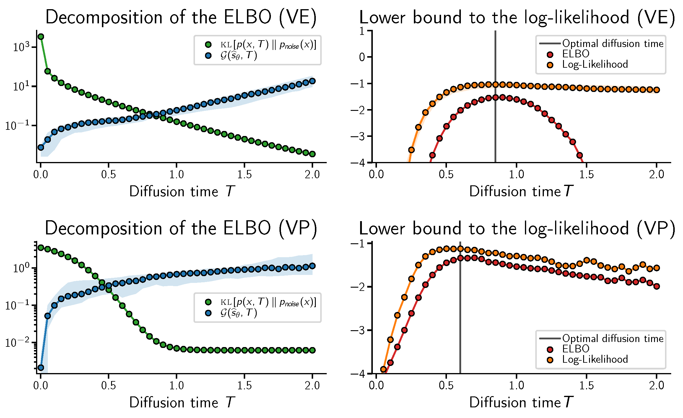
2.2. The Tradeoff on Diffusion Time

| Diffusion Process | |||
|---|---|---|---|
| Variance Exploding | , | , | |
| Variance Preserving | , | , |
2.3. Is There an Optimal Diffusion Time?
2.4. Relation with Diffusion Process Noise Schedule
2.5. Relation with Literature on Bounds and Goodness of Score Assumptions
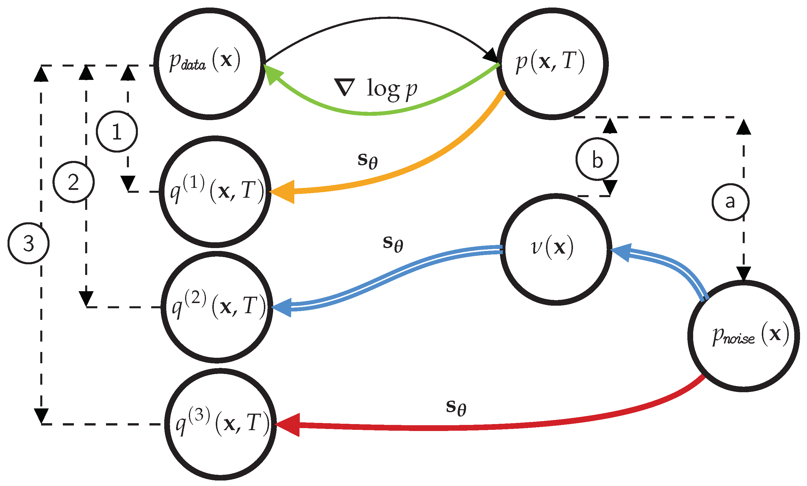
3. A New, Practical Method for Decreasing Diffusion Times
3.1. Auxiliary Model Fitting and Guarantees
3.2. Comparison with Schrödinger Bridges
3.3. An Extension for Density Estimation
4. Experiments
5. Conclusions
Author Contributions
Funding
Data Availability Statement
Conflicts of Interest
Appendix A. Generic Definitions and Assumptions
Appendix B. Deriving Equation (4) from [32]
Appendix C. Proof of Equation (5)
Appendix D. Proof of Equation (8)
Appendix E. Proof of Lemma 1
Appendix E.1. The Variance Preserving (VP) Convergence
Appendix E.2. The Variance Exploding (VE) Convergence
Appendix F. Proof for the Optimal Score Gap Term, Section 2.2
Appendix G. Proof of Section 2.3
Appendix H. Optimization of T ★
Appendix I. Proof of Proposition 2
Appendix J. Invariance to Noise Schedule
Appendix J.1. Preliminaries
Appendix J.2. Different Noise Schedules
Appendix K. Experimental Details
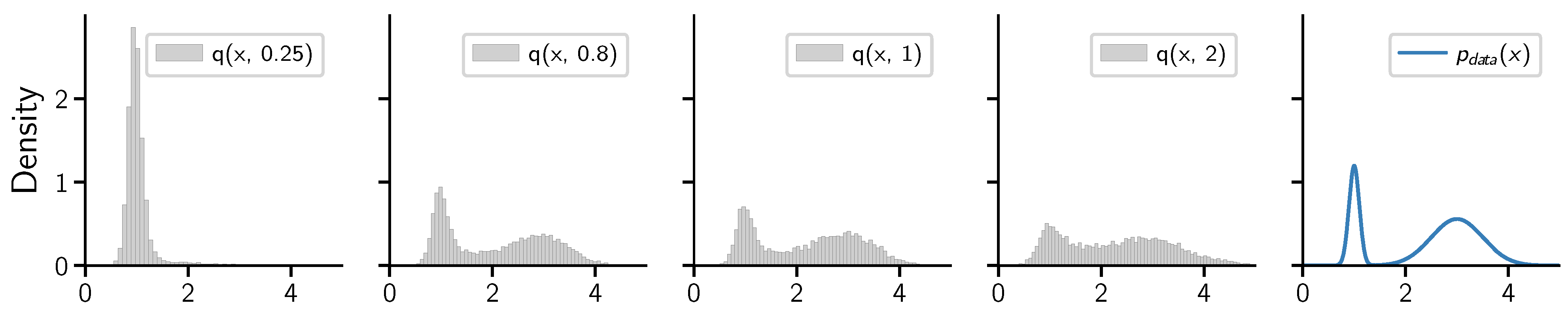
Appendix K.1. Toy Example Details

Appendix K.2. Section 4 Details
Appendix K.3. Varying T
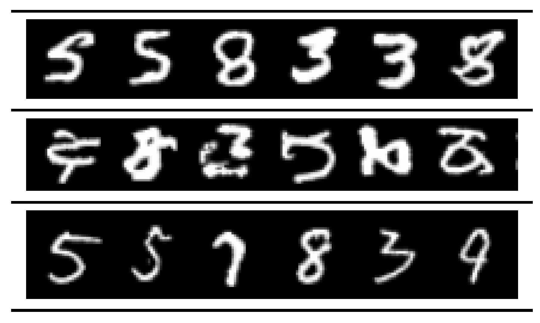
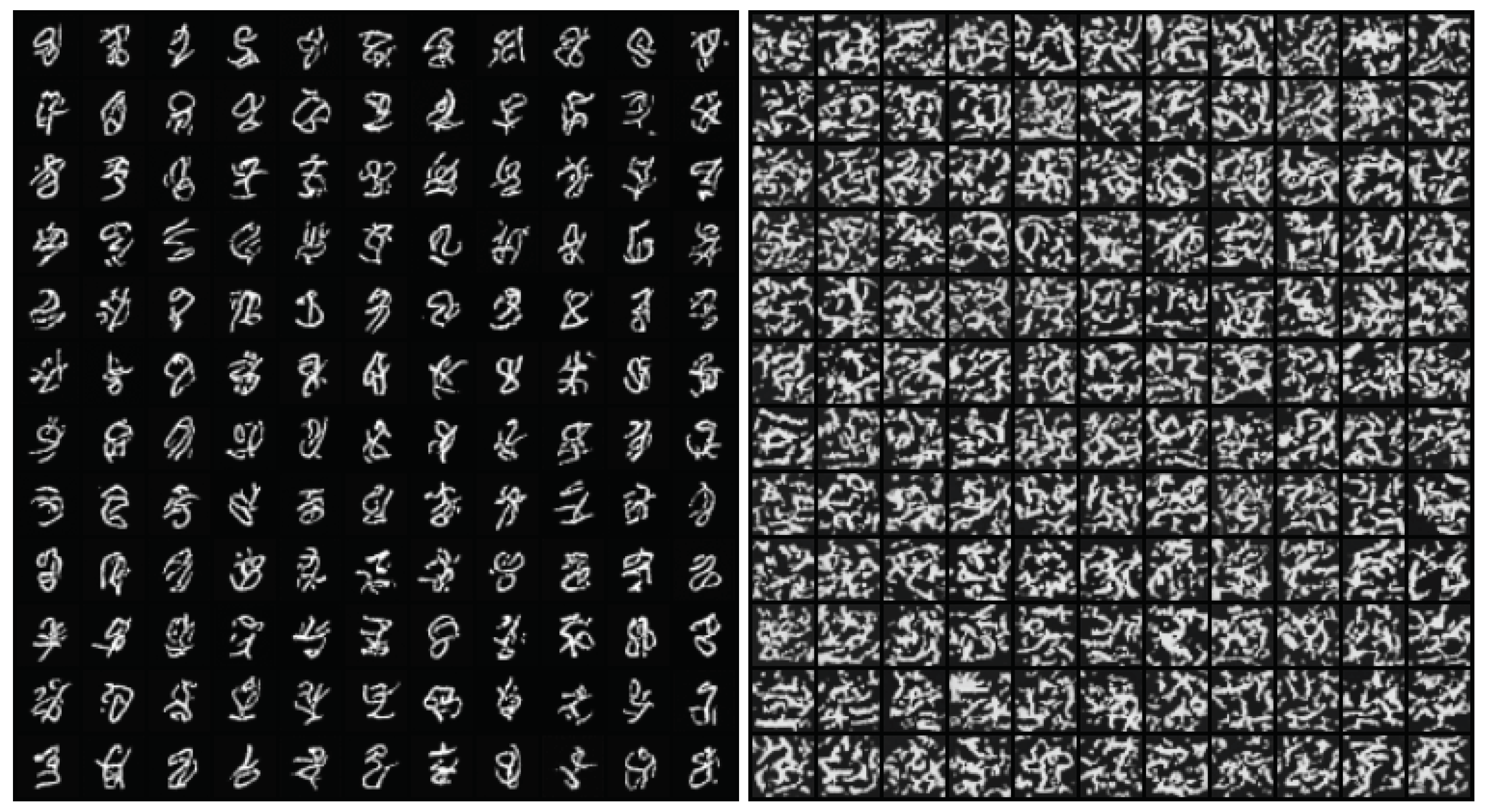
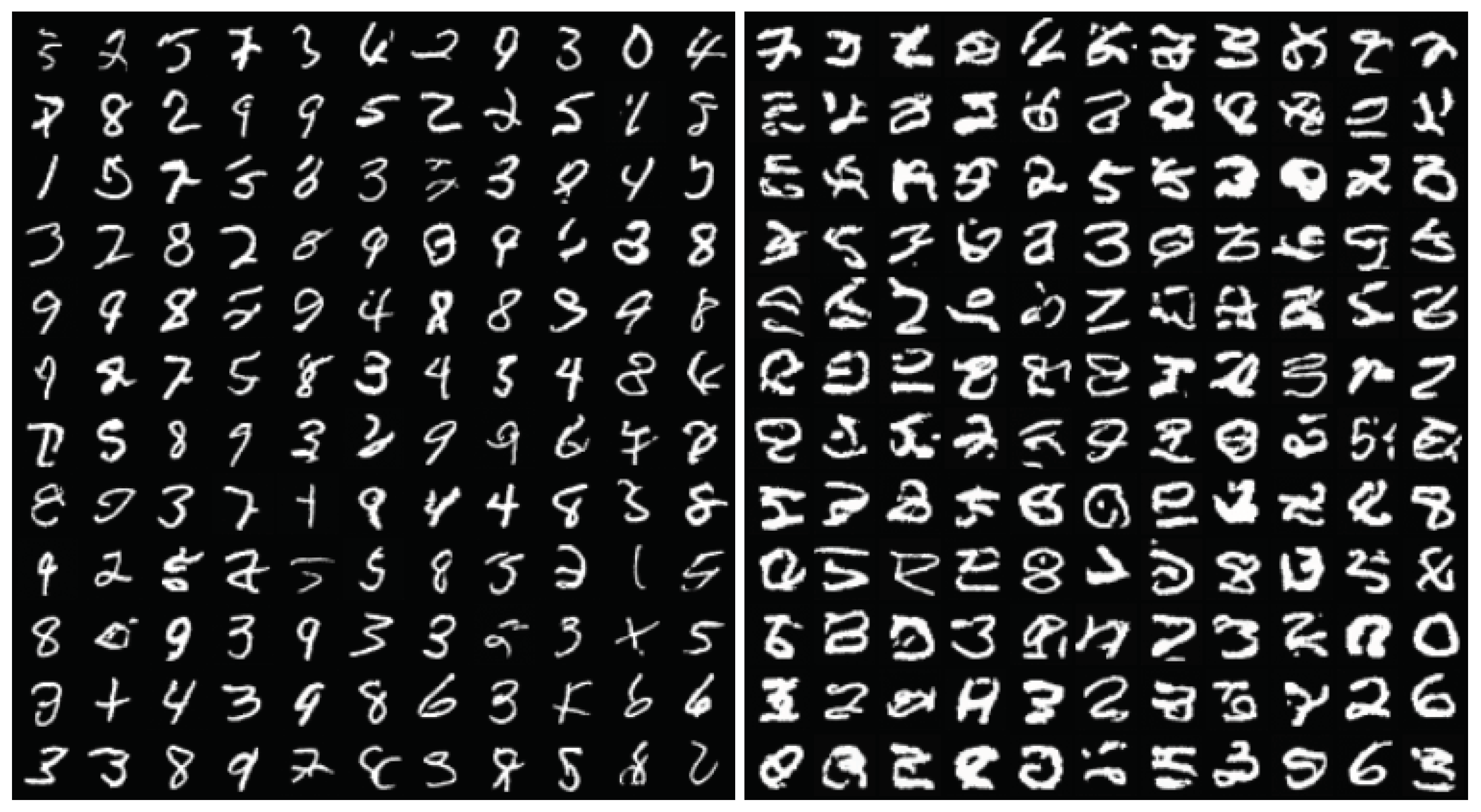
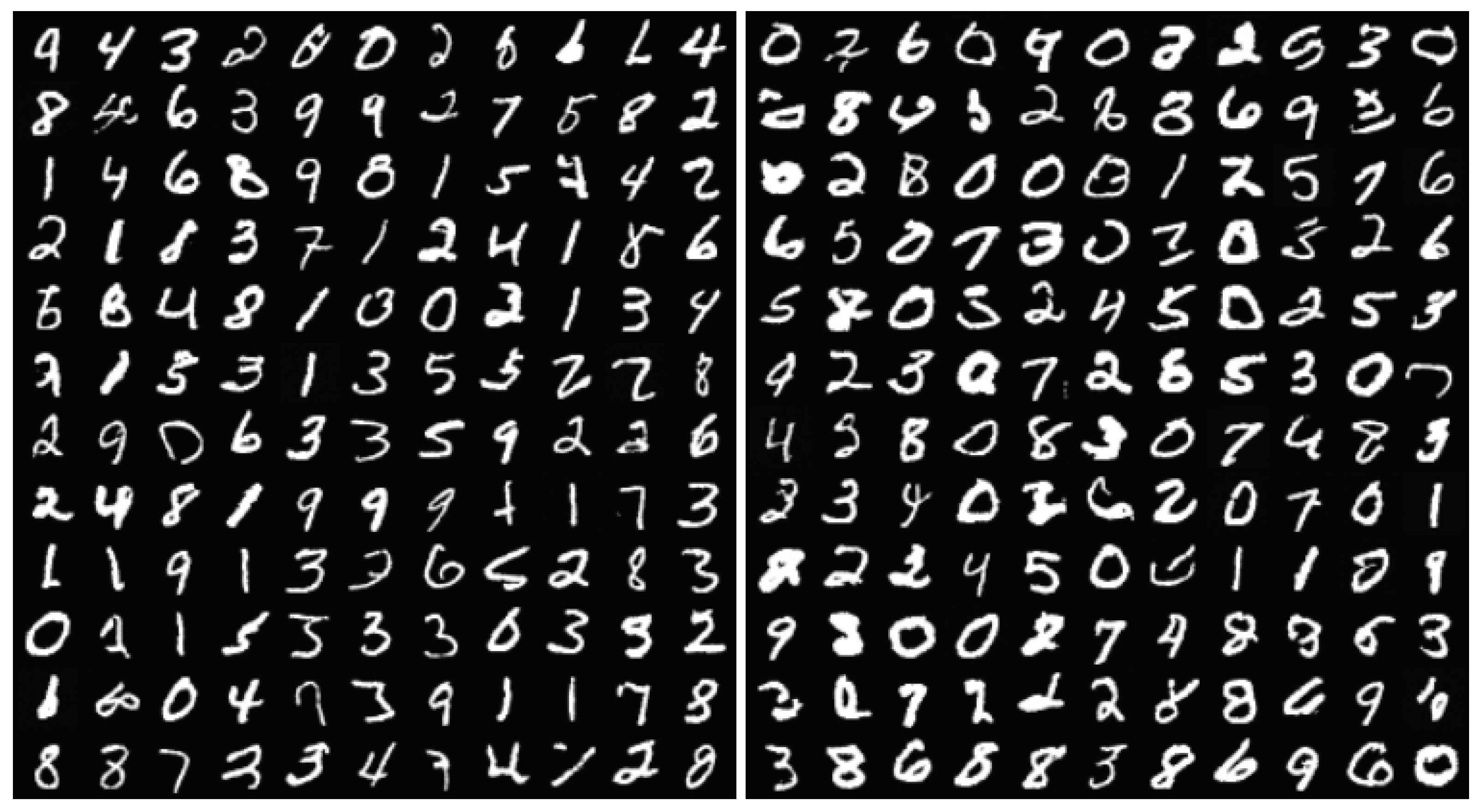
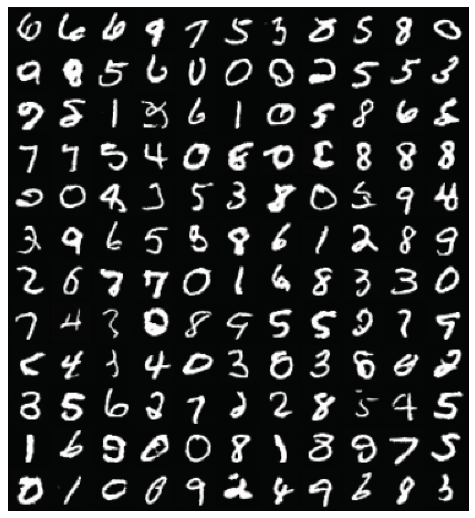
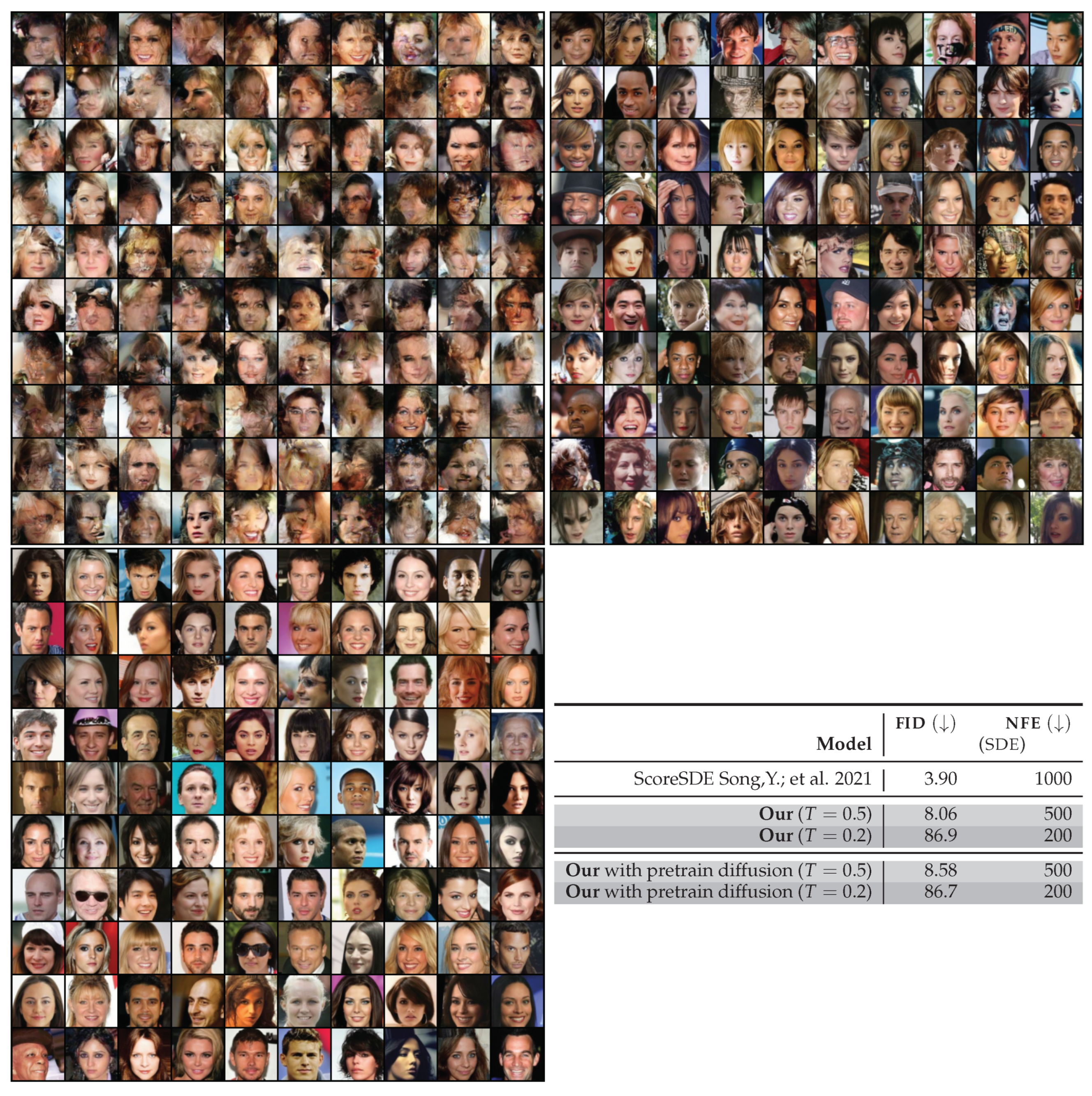
Appendix L. Non-Curated Samples


References
- Sohl-Dickstein, J.; Weiss, E.; Maheswaranathan, N.; Ganguli, S. Deep unsupervised learning using nonequilibrium thermodynamics. In Proceedings of the International Conference on Machine Learning, Lille, France, 6–11 July 2015. [Google Scholar]
- Song, Y.; Ermon, S. Generative Modeling by Estimating Gradients of the Data Distribution. In Proceedings of the Advances in Neural Information Processing Systems, Vancouver, BC, Canada, 8–14 December 2019. [Google Scholar]
- Song, Y.; Sohl-Dickstein, J.; Kingma, D.P.; Kumar, A.; Ermon, S.; Poole, B. Score-Based Generative Modeling through Stochastic Differential Equations. In Proceedings of the International Conference on Learning Representations, Virtual, 30 April–3 May 2021. [Google Scholar]
- Vahdat, A.; Kreis, K.; Kautz, J. Score-based Generative Modeling in Latent Space. In Proceedings of the Advances in Neural Information Processing Systems, Virtual, 6–14 December 2021. [Google Scholar]
- Kingma, D.; Salimans, T.; Poole, B.; Ho, J. Variational Diffusion Models. In Proceedings of the Advances in Neural Information Processing Systems, Virtual, 6–14 December 2021. [Google Scholar]
- Ho, J.; Jain, A.; Abbeel, P. Denoising Diffusion Probabilistic Models. In Proceedings of the Advances in Neural Information Processing Systems, Online, 6–12 December 2020. [Google Scholar]
- Song, J.; Meng, C.; Ermon, S. Denoising Diffusion Implicit Models. In Proceedings of the International Conference on Learning Representations, Virtual, 30 April–3 May 2021. [Google Scholar]
- Kong, Z.; Ping, W.; Huang, J.; Zhao, K.; Catanzaro, B. DiffWave: A Versatile Diffusion Model for Audio Synthesis. In Proceedings of the International Conference on Learning Representations, Virtual, 30 April–3 May 2021. [Google Scholar]
- Lee, S.G.; Kim, H.; Shin, C.; Tan, X.; Liu, C.; Meng, Q.; Qin, T.; Chen, W.; Yoon, S.; Liu, T.Y. PriorGrad: Improving Conditional Denoising Diffusion Models with Data-Dependent Adaptive Prior. In Proceedings of the International Conference on Learning Representations, Virtual, 25–29 April 2022. [Google Scholar]
- Dhariwal, P.; Nichol, A. Diffusion Models Beat GANs on Image Synthesis. In Proceedings of the Advances in Neural Information Processing Systems, Virtual, 6–14 December 2021. [Google Scholar]
- Nichol, A.Q.; Dhariwal, P. Improved Denoising Diffusion Probabilistic Models. In Proceedings of the International Conference on Machine Learning, Virtual, 18–24 July 2021. [Google Scholar]
- Tashiro, Y.; Song, J.; Song, Y.; Ermon, S. CSDI: Conditional Score-based Diffusion Models for Probabilistic Time Series Imputation. In Proceedings of the Advances in Neural Information Processing Systems, Virtual, 6–14 December 2021. [Google Scholar]
- Goodfellow, I.; Pouget-Abadie, J.; Mirza, M.; Xu, B.; Warde-Farley, D.; Ozair, S.; Courville, A.; Bengio, Y. Generative Adversarial Nets. In Proceedings of the Advances in Neural Information Processing Systems, Montreal, QC, Canada, 8–13 December 2014. [Google Scholar]
- Kingma, D.P.; Salimans, T.; Jozefowicz, R.; Chen, X.; Sutskever, I.; Welling, M. Improved Variational Inference with Inverse Autoregressive Flow. In Proceedings of the Advances in Neural Information Processing Systems 29, Barcelona, Spain, 5–10 December 2016. [Google Scholar]
- Kingma, D.P.; Welling, M. Auto-Encoding Variational Bayes. In Proceedings of the International Conference on Learning Representations, Banff, AB, Canada, 14–16 April 2014. [Google Scholar]
- Tran, B.H.; Rossi, S.; Milios, D.; Michiardi, P.; Bonilla, E.V.; Filippone, M. Model Selection for Bayesian Autoencoders. In Proceedings of the Advances in Neural Information Processing Systems, Virtual, 6–14 December 2021. [Google Scholar]
- Anderson, B.D. Reverse-Time Diffusion Equation Models. Stoch. Process. Their Appl. 1982, 12, 313–326. [Google Scholar] [CrossRef]
- Song, Y.; Durkan, C.; Murray, I.; Ermon, S. Maximum Likelihood Training of Score-Based Diffusion Models. In Proceedings of the Advances in Neural Information Processing Systems, Virtual, 6–14 December 2021. [Google Scholar]
- Särkkä, S.; Solin, A. Applied Stochastic Differential Equations; Institute of Mathematical Statistics Textbooks, Cambridge University Press: Cambridge, UK, 2019. [Google Scholar] [CrossRef]
- Zheng, H.; He, P.; Chen, W.; Zhou, M. Truncated Diffusion Probabilistic Models. CoRR 2022. abs/2202.09671. Available online: http://xxx.lanl.gov/abs/2202.09671 (accessed on 28 March 2023).
- Austin, J.; Johnson, D.D.; Ho, J.; Tarlow, D.; van den Berg, R. Structured Denoising Diffusion Models in Discrete State-Spaces. In Proceedings of the Advances in Neural Information Processing Systems, Virtual, 6–14 December 2021. [Google Scholar]
- Jolicoeur-Martineau, A.; Li, K.; Piché-Taillefer, R.; Kachman, T.; Mitliagkas, I. Gotta Go Fast When Generating Data with Score-Based Models. CoRR 2021. abs/2105.14080. Available online: http://xxx.lanl.gov/abs/2105.14080 (accessed on 28 March 2023).
- Salimans, T.; Ho, J. Progressive Distillation for Fast Sampling of Diffusion Models. In Proceedings of the International Conference on Learning Representations, Virtual, 25–29 April 2022. [Google Scholar]
- Xiao, Z.; Kreis, K.; Vahdat, A. Tackling the Generative Learning Trilemma with Denoising Diffusion GANs. In Proceedings of the International Conference on Learning Representations, Virtual, 25–29 April 2022. [Google Scholar]
- Watson, D.; Ho, J.; Norouzi, M.; Chan, W. Learning to Efficiently Sample from Diffusion Probabilistic Models. CoRR 2021. abs/2106.03802. Available online: http://xxx.lanl.gov/abs/2106.03802 (accessed on 28 March 2023).
- Dockhorn, T.; Vahdat, A.; Kreis, K. Score-Based Generative Modeling with Critically-Damped Langevin Diffusion. In Proceedings of the International Conference on Learning Representations, Virtual, 25–29 April 2022. [Google Scholar]
- Rombach, R.; Blattmann, A.; Lorenz, D.; Esser, P.; Ommer, B. High-Resolution Image Synthesis with Latent Diffusion Models. In Proceedings of the IEEE Conference on Computer Vision and Pattern Recognition, New Orleans, LA, USA, 19–20 June 2022. [Google Scholar]
- Bao, F.; Li, C.; Zhu, J.; Zhang, B. Analytic-DPM: An Analytic Estimate of the Optimal Reverse Variance in Diffusion Probabilistic Models. In Proceedings of the International Conference on Learning Representations, Virtual, 25–29 April 2022. [Google Scholar]
- De Bortoli, V.; Thornton, J.; Heng, J.; Doucet, A. Diffusion Schrödinger Bridge with Applications to Score-Based Generative Modeling. In Proceedings of the Advances in Neural Information Processing Systems, Virtual, 6–14 December 2021. [Google Scholar]
- De Bortoli, V. Convergence of denoising diffusion models under the manifold hypothesis. arXiv 2022, arXiv:2208.05314. [Google Scholar]
- Lee, H.; Lu, J.; Tan, Y. Convergence for score-based generative modeling with polynomial complexity. arXiv 2022, arXiv:2206.06227. [Google Scholar]
- Huang, C.W.; Lim, J.H.; Courville, A.C. A Variational Perspective on Diffusion-Based Generative Models and Score Matching. In Proceedings of the Advances in Neural Information Processing Systems, Virtual, 6–14 December 2021. [Google Scholar]
- Villani, C. Optimal Transport: Old and New; Springer: Berlin/Heidelberg, Germany, 2009; Volume 338. [Google Scholar]
- Chen, S.; Chewi, S.; Li, J.; Li, Y.; Salim, A.; Zhang, A.R. Sampling is as easy as learning the score: Theory for diffusion models with minimal data assumptions. arXiv 2022, arXiv:2209.11215. [Google Scholar]
- Chen, Y.; Georgiou, T.T.; Pavon, M. Stochastic control liaisons: Richard sinkhorn meets gaspard monge on a schrodinger bridge. SIAM Rev. 2021, 63, 249–313. [Google Scholar] [CrossRef]
- Chen, T.; Liu, G.H.; Theodorou, E. Likelihood Training of Schrödinger Bridge using Forward-Backward SDEs Theory. In Proceedings of the International Conference on Learning Representations, Virtual, 25–29 April 2022. [Google Scholar]
- Chen, R.T.Q.; Rubanova, Y.; Bettencourt, J.; Duvenaud, D.K. Neural Ordinary Differential Equations. In Proceedings of the Advances in Neural Information Processing Systems, Montreal, QC, Canada, 3–8 December 2018. [Google Scholar]
- Grathwohl, W.; Chen, R.T.Q.; Bettencourt, J.; Duvenaud, D. Scalable Reversible Generative Models with Free-form Continuous Dynamics. In Proceedings of the International Conference on Learning Representations, New Orleans, LA, USA, 6–9 May 2019. [Google Scholar]
- Kynkäänniemi, T.; Karras, T.; Aittala, M.; Aila, T.; Lehtinen, J. The Role of ImageNet Classes in Fréchet Inception Distance. CoRR 2022. abs/2203.06026. Available online: http://xxx.lanl.gov/abs/2203.06026 (accessed on 28 March 2023).
- Theis, L.; van den Oord, A.; Bethge, M. A Note on the Evaluation of Generative Models. In Proceedings of the International Conference on Learning Representations, San Juan, Puerto Rico, 2–4 May 2016. [Google Scholar]
- Rasmussen, C. The Infinite Gaussian Mixture Model. In Proceedings of the Advances in Neural Information Processing Systems, Denver, CO, USA, 29 November–4 December 1999. [Google Scholar]
- Görür, D.; Edward Rasmussen, C. Dirichlet Process Gaussian Mixture Models: Choice of the Base Distribution. J. Comput. Sci. Technol. 2010, 25, 653–664. [Google Scholar] [CrossRef]
- Kingma, D.P.; Dhariwal, P. Glow: Generative Flow with Invertible 1 × 1 Convolutions. In Proceedings of the Advances in Neural Information Processing Systems, Montreal, QC, Canada, 3–8 December 2018. [Google Scholar]
- Hoogeboom, E.; Gritsenko, A.A.; Bastings, J.; Poole, B.; van den Berg, R.; Salimans, T. Autoregressive Diffusion Models. In Proceedings of the International Conference on Learning Representations, Virtual, 25–29 April 2022. [Google Scholar]
- Kloeden, P.E.; Platen, E. Numerical Solution of Stochastic Differential Equations; Springer: Berlin/Heidelberg, Germany, 1995. [Google Scholar]
- Karras, T.; Aittala, M.; Aila, T.; Laine, S. Elucidating the Design Space of Diffusion-Based Generative Models. arXiv 2022, arXiv:2206.00364. [Google Scholar]


| Dataset | Time T | BPD (↓) |
|---|---|---|
| MNIST | ||
| CIFAR10 | ||
| NFE (↓) | BPD (↓) | ||
| Model | (ODE) | ||
| ScoreSDE | 300 | ||
| ScoreSDE () | 258 | ||
| Our () | 258 | (S) | |
| ScoreSDE () | 235 | ||
| Our () | 235 | (S) | |
| ScoreSDE () | 191 | ||
| Our () | 191 | (S) | |
| FID | BPD | NFE | NFE | |
| Model | (SDE) | (ODE) | ||
| ScoreSDE [3] | 1000 | 221 | ||
| ScoreSDE () | 600 | 200 | ||
| ScoreSDE () | 400 | 187 | ||
| ScoreSDE () | 200 | 176 | ||
| Our () | 600 | 200 | ||
| Our () | 400 | 187 | ||
| Our () | 200 | 176 | ||
| ARDM [44] | − | 3072 | ||
| VDM [5] | 1000 | |||
| D3PMs [21] | 1000 | |||
| DDPM [6] | 1000 | |||
| Gotta Go Fast [22] | − | 180 | ||
| LSGM [4] | ||||
| ARDM-P [44] | − |
Disclaimer/Publisher’s Note: The statements, opinions and data contained in all publications are solely those of the individual author(s) and contributor(s) and not of MDPI and/or the editor(s). MDPI and/or the editor(s) disclaim responsibility for any injury to people or property resulting from any ideas, methods, instructions or products referred to in the content. |
© 2023 by the authors. Licensee MDPI, Basel, Switzerland. This article is an open access article distributed under the terms and conditions of the Creative Commons Attribution (CC BY) license (https://creativecommons.org/licenses/by/4.0/).
Share and Cite
Franzese, G.; Rossi, S.; Yang, L.; Finamore, A.; Rossi, D.; Filippone, M.; Michiardi, P. How Much Is Enough? A Study on Diffusion Times in Score-Based Generative Models. Entropy 2023, 25, 633. https://doi.org/10.3390/e25040633
Franzese G, Rossi S, Yang L, Finamore A, Rossi D, Filippone M, Michiardi P. How Much Is Enough? A Study on Diffusion Times in Score-Based Generative Models. Entropy. 2023; 25(4):633. https://doi.org/10.3390/e25040633
Chicago/Turabian StyleFranzese, Giulio, Simone Rossi, Lixuan Yang, Alessandro Finamore, Dario Rossi, Maurizio Filippone, and Pietro Michiardi. 2023. "How Much Is Enough? A Study on Diffusion Times in Score-Based Generative Models" Entropy 25, no. 4: 633. https://doi.org/10.3390/e25040633
APA StyleFranzese, G., Rossi, S., Yang, L., Finamore, A., Rossi, D., Filippone, M., & Michiardi, P. (2023). How Much Is Enough? A Study on Diffusion Times in Score-Based Generative Models. Entropy, 25(4), 633. https://doi.org/10.3390/e25040633