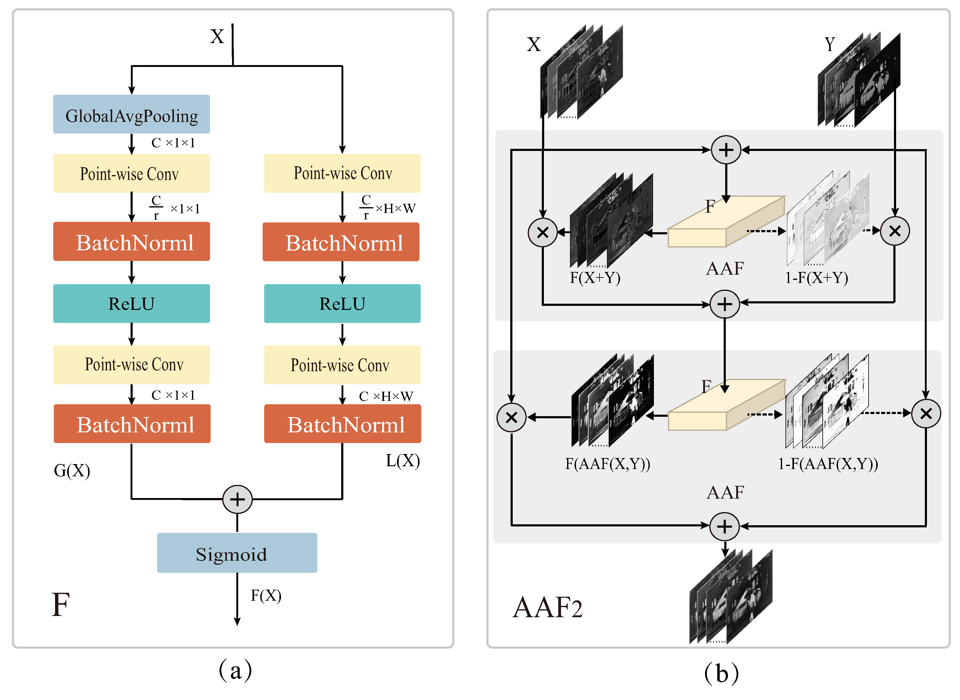
Figure 1.
Schematic of AAF strategy. (a) The multiscale channel attention module F. (b) The two-layer iterative AAF module.
Figure 1.
Schematic of AAF strategy. (a) The multiscale channel attention module F. (b) The two-layer iterative AAF module.
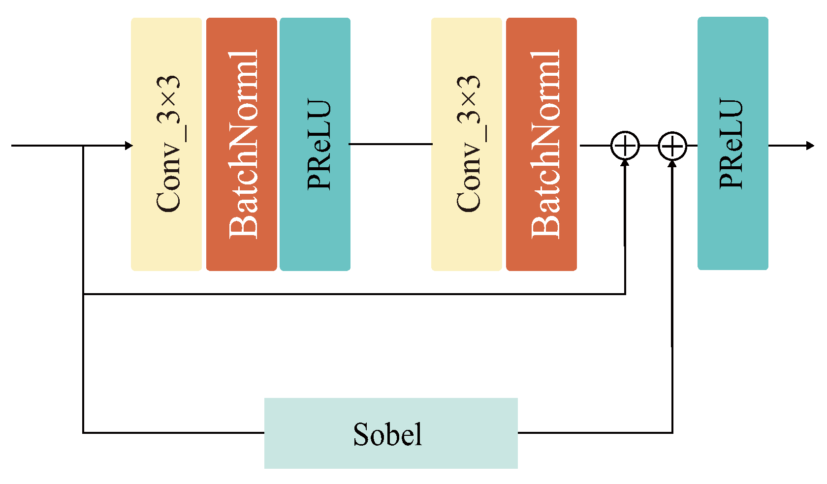
Figure 2.
Specific design of the structural residual module (SRM). Structural residual parallel Sobel operator consisting of two 3 × 3 convolution kernels, two batch normalization layer, and two PReLU activation function.
Figure 2.
Specific design of the structural residual module (SRM). Structural residual parallel Sobel operator consisting of two 3 × 3 convolution kernels, two batch normalization layer, and two PReLU activation function.
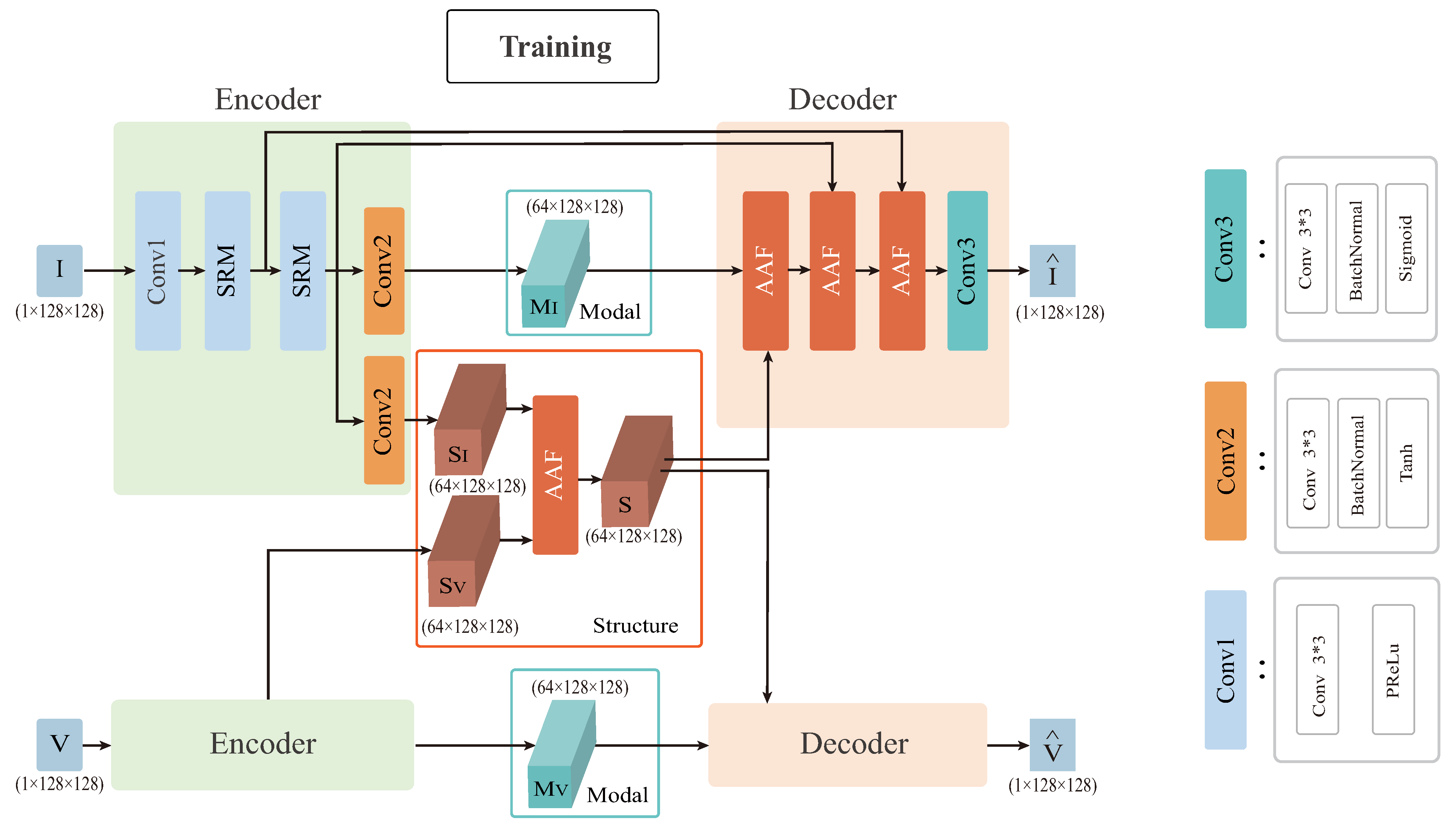
Figure 3.
Schematic diagram of the overall AAF framework. SRM is the structural residual module and AAF is attention-based adaptive fusion module. conv1 consists of a 3 × 3 convolution kernel, a PReLU activation function, conv2 consists of a 3 × 3 convolution kernel, a batch normalization layer, a Tanh activation function, and conv3 consists of a 3 × 3 convolution kernel, a batch normalization layer, a Sigmoid activation function.
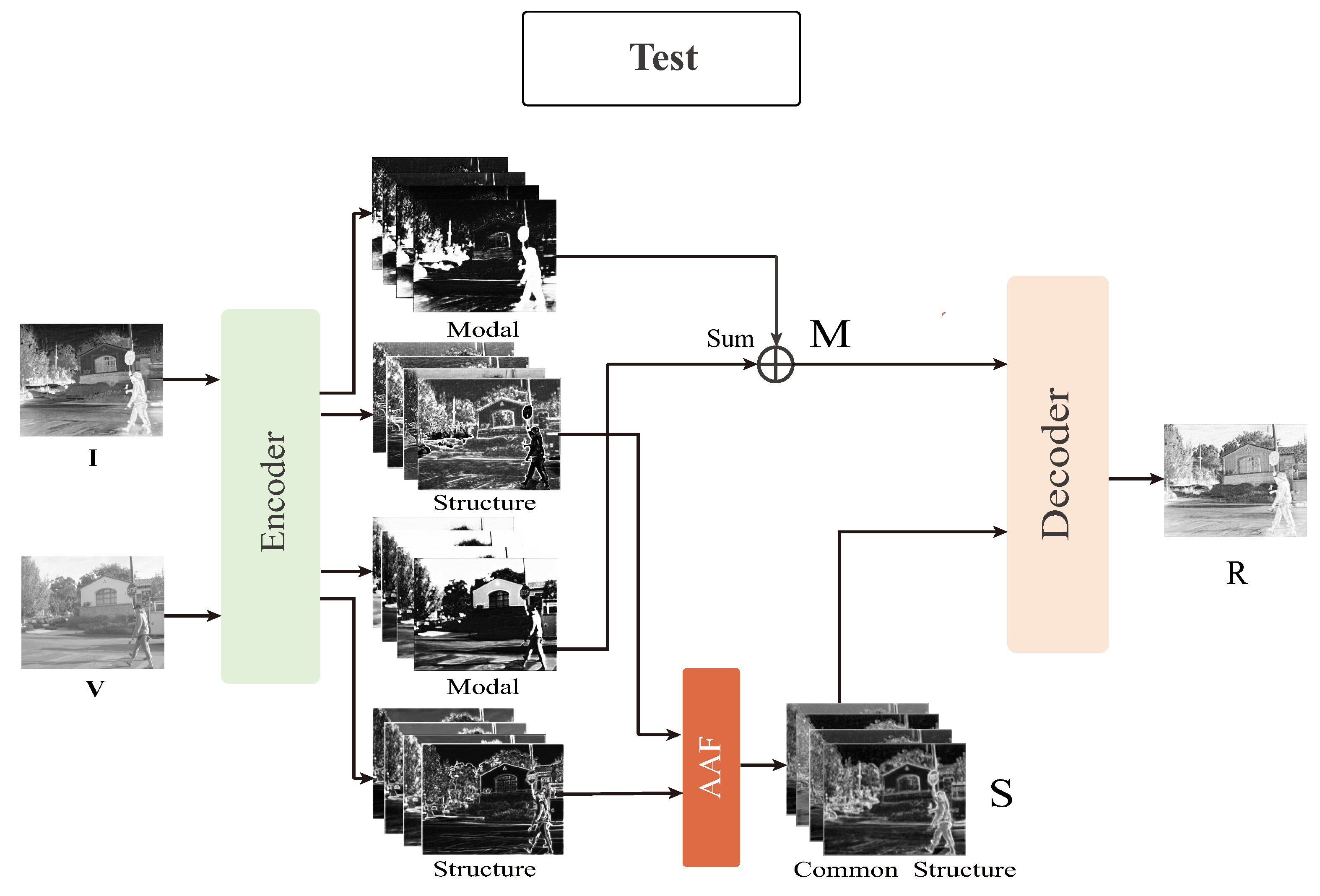
Figure 4.
Schematic diagram of AAF test framework. M represents the added modal features and R is the fused image.
Figure 4.
Schematic diagram of AAF test framework. M represents the added modal features and R is the fused image.
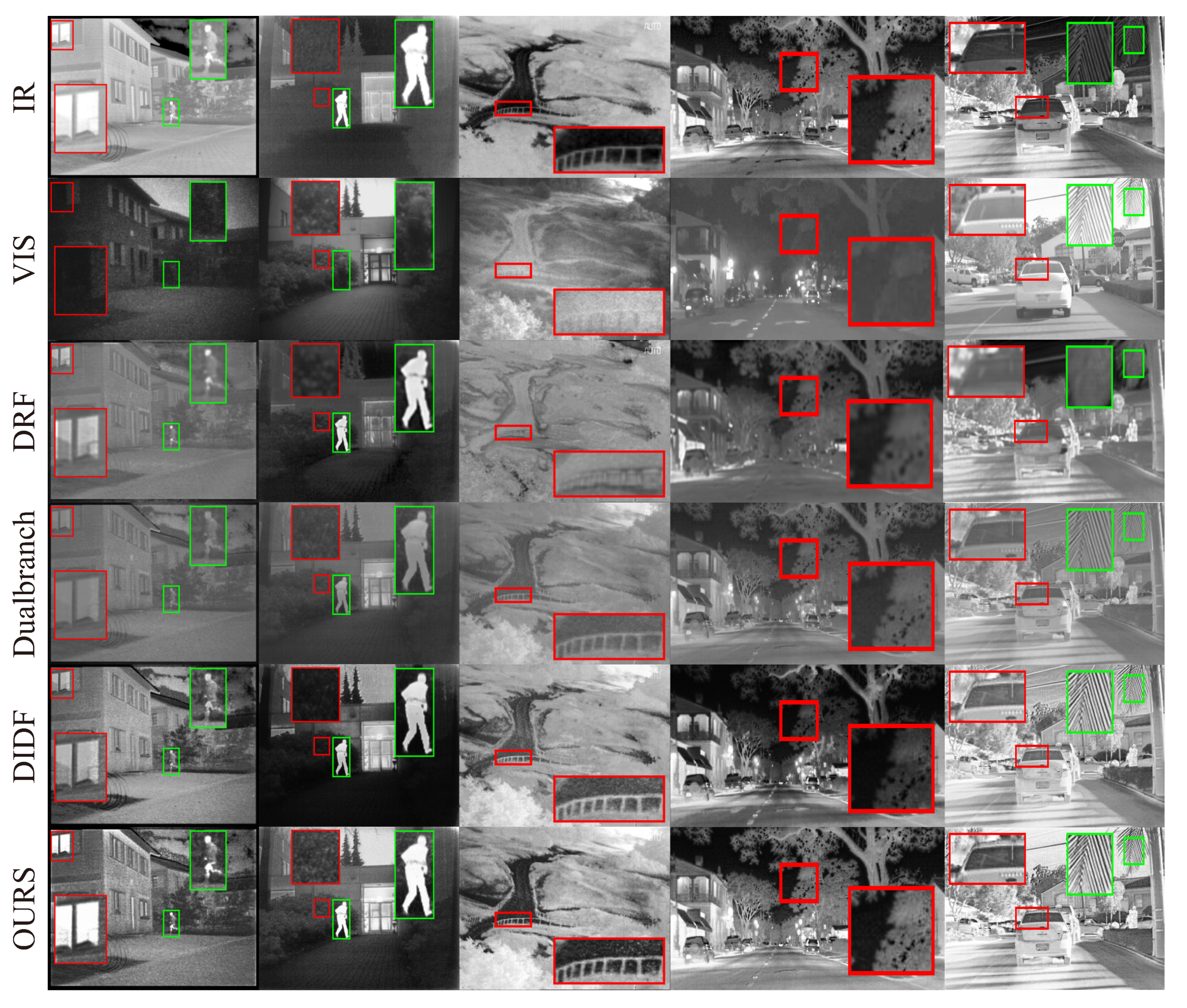
Figure 5.
Qualitative experimental result comparison of the AAF model with DRF, Dual-branch Net and DIDFuse on the TNO and RoadScene datasets. The first two rows are infrared and visible images, and the following are the fused images by DRF, Dualbranch, DIDFuse, and our AAF model in order. Three columns on the left: TNO dataset, two columns on the right: RoadScene dataset.
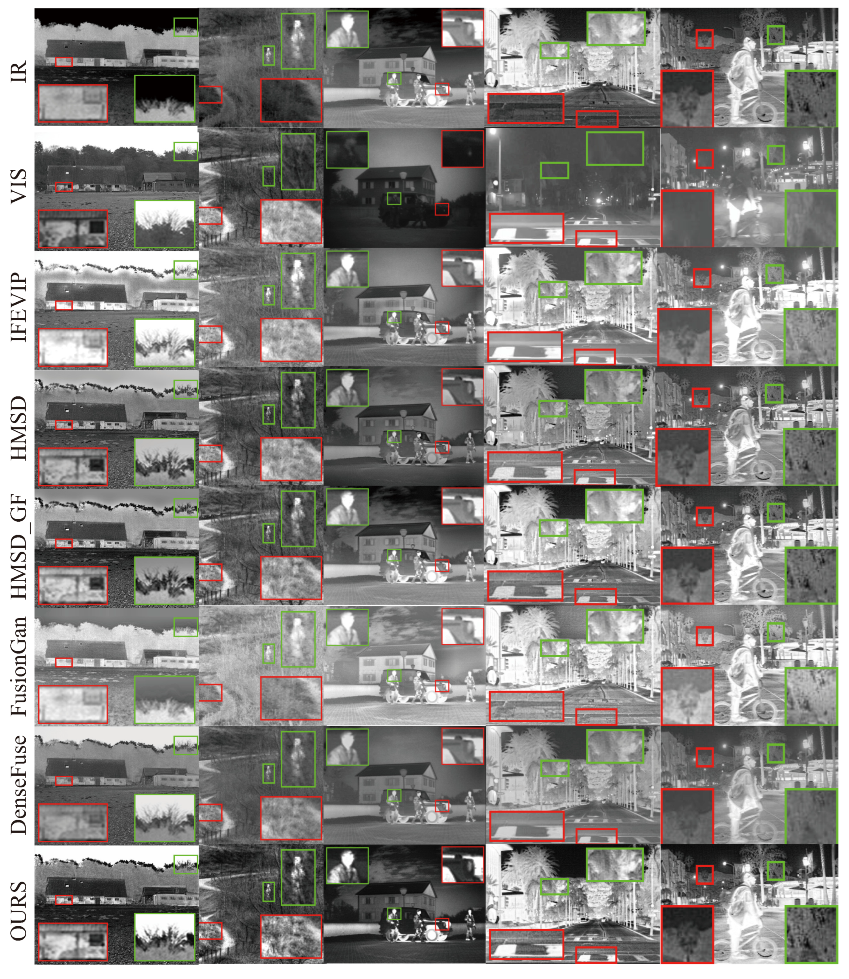
Figure 6.
Qualitative comparison of AAF model with five state-of-the-art IVIF methods on the TNO and RoadScene test datasets. The first two top rows are the infrared and visible images, and the following are the fused images by IFEVIP, HMSD, HMSD_GF, FusionGAN, DenseFuse, and our AAF model. The three columns on the left: the TNO dataset, and the two columns on the right: the RoadScene dataset.
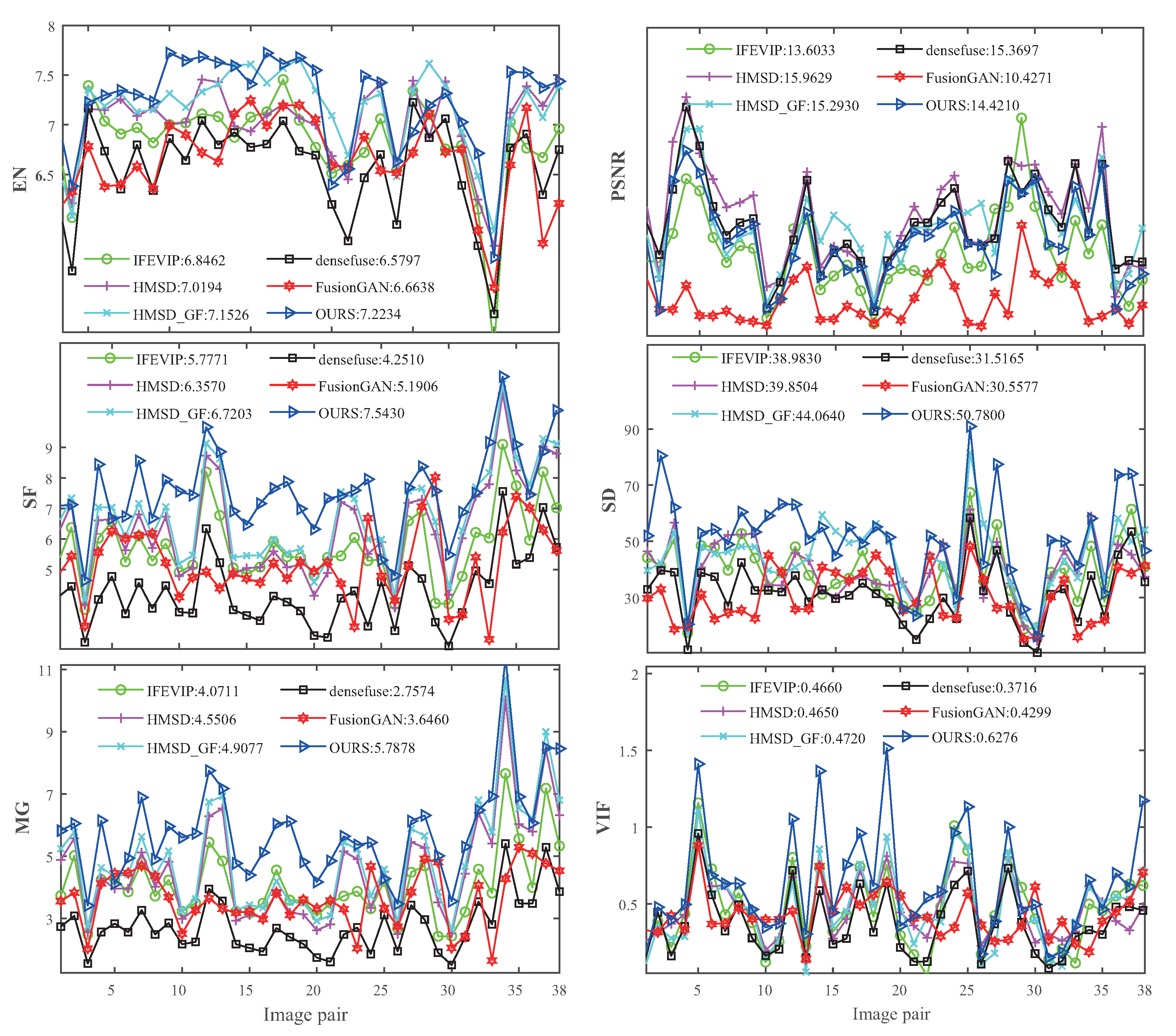
Figure 7.
Quantitative comparison results of the AAF model with five state-of-the-art methods on six metrics for the TNO test dataset.
Figure 7.
Quantitative comparison results of the AAF model with five state-of-the-art methods on six metrics for the TNO test dataset.
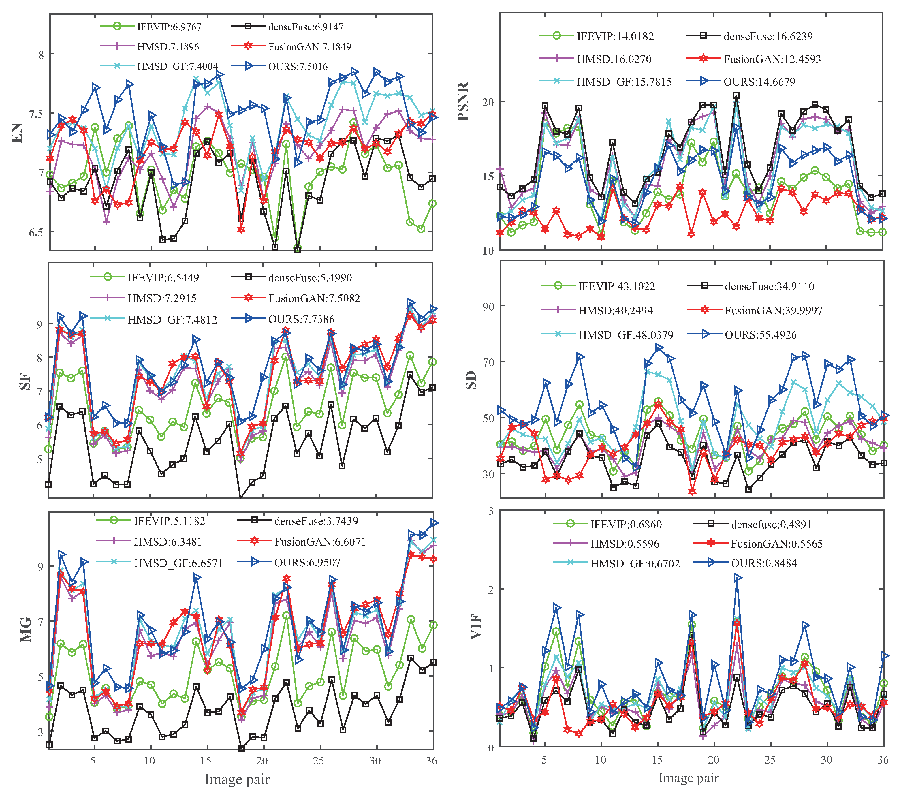
Figure 8.
Quantitative comparison results of the AAF model with five state-of-the-art methods on six metrics for the RoadScene test dataset.
Figure 8.
Quantitative comparison results of the AAF model with five state-of-the-art methods on six metrics for the RoadScene test dataset.
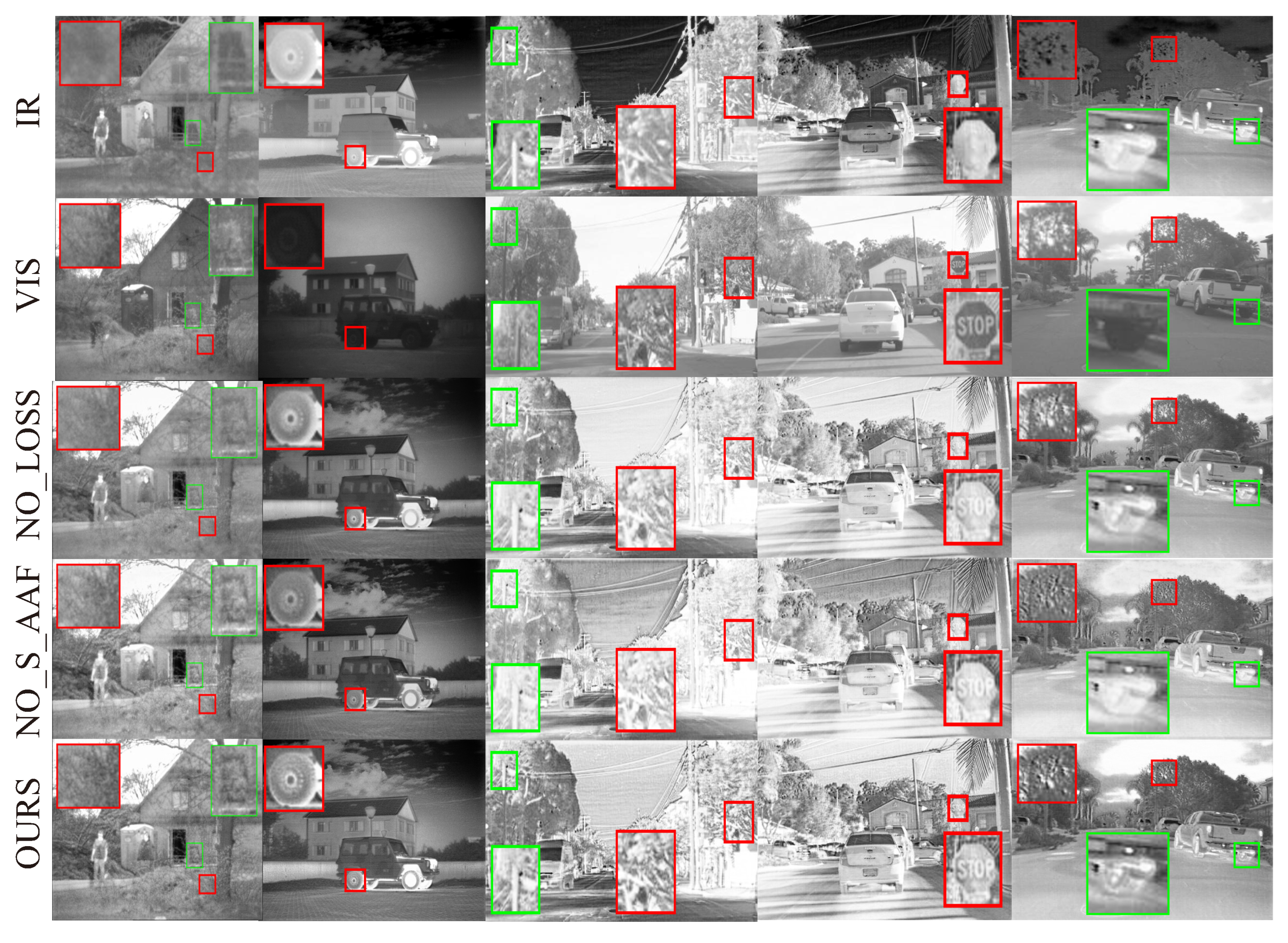
Figure 9.
The two columns on the left: TNO test dataset, and the three columns on the right: RoadScene test dataset. The first two top rows are the source images, followed by the fused images by the NO_Loss model and NO_S_AAF model and the full model, respectively.
Figure 9.
The two columns on the left: TNO test dataset, and the three columns on the right: RoadScene test dataset. The first two top rows are the source images, followed by the fused images by the NO_Loss model and NO_S_AAF model and the full model, respectively.
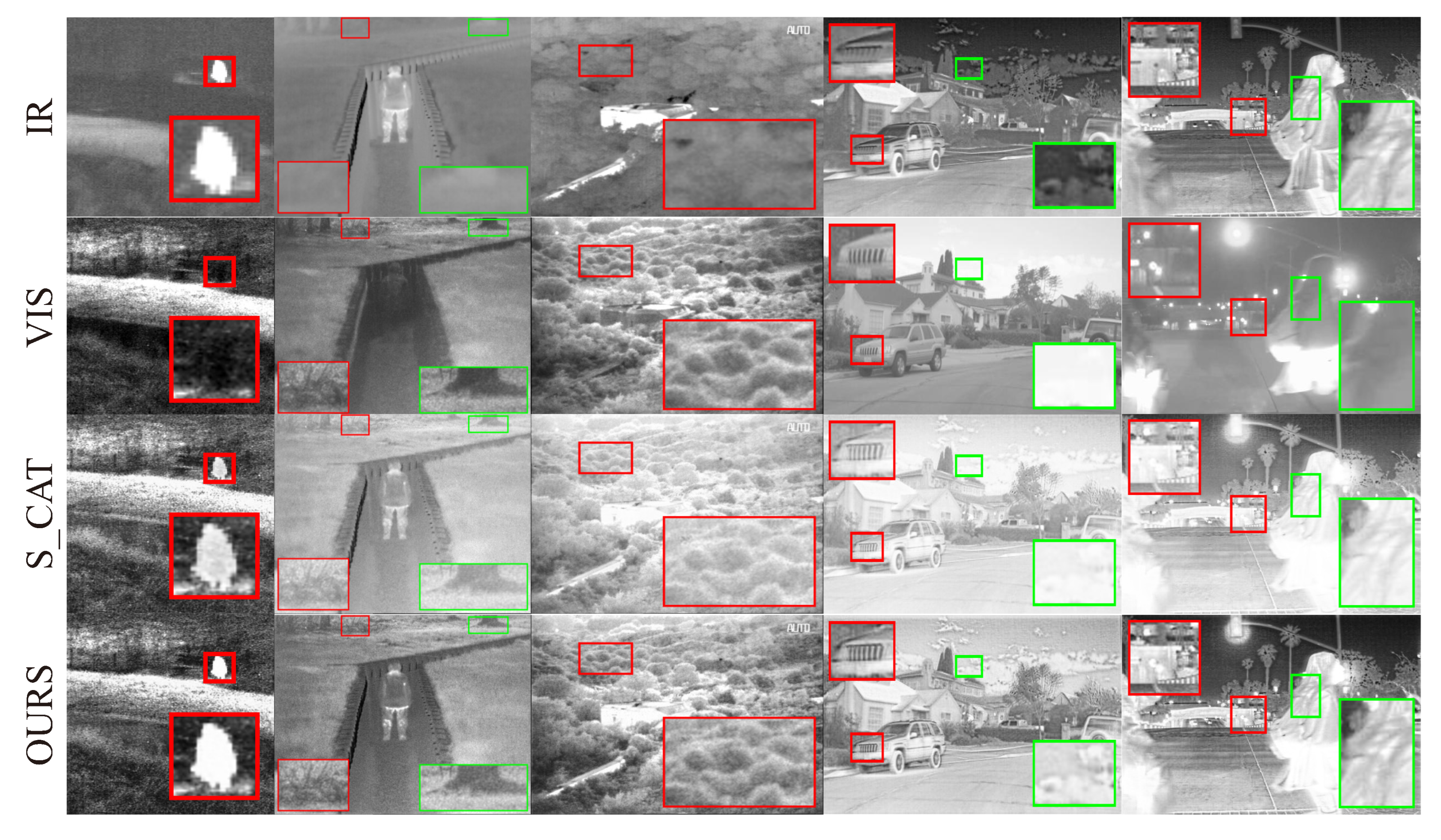
Figure 10.
Qualitative ablation study of AAF strategy. The three columns on the left: TNO test dataset and the two columns on the right: RoadScene test dataset. The first two top rows are the source images, and the following are the fusion images by the model with concatenation strategy and those by the AAF model.
Table 1.
Feature fusion formulas for different fusion strategies. G(·) denotes the weight generation module and ⊗ denotes the matrix multiplication.
Table 1.
Feature fusion formulas for different fusion strategies. G(·) denotes the weight generation module and ⊗ denotes the matrix multiplication.
| Context-Aware | Type | Formulation | Example |
|---|
| | Addition | X + Y | DRF [17], Dual-branch [19] |
| | Concatenation | | DIDFuse [20], CUFD [18] |
| None | Average | | TIF [33] |
| | Choose-max | | GFF [11], IFCNN [24] |
| | Max- | | NGDC [13] |
| | -norm | | DenseFuse [26] |
| Fully | Soft Selection | G(X + Y) ⊗ X + (1 − G(X + Y)) ⊗ Y | SKNet [34] |
Table 2.
Quantitative comparison of AAF model with DRF, Dual-branch Net and DIDFuse on the TNO dataset. The best, second best and third best values are indicated in black bold, red and blue, respectively.
Table 2.
Quantitative comparison of AAF model with DRF, Dual-branch Net and DIDFuse on the TNO dataset. The best, second best and third best values are indicated in black bold, red and blue, respectively.
| Methods | EN | SF | MG | PSNR | SD | VIF |
|---|
| DRF | 6.4773 | 3.0594 | 2.1140 | 14.0305 | 28.2402 | 0.3480 |
| Dualbranch | 6.3507 | 3.5606 | 2.3751 | 15.5899 | 24.4902 | 0.2988 |
| DIDF | 7.1002 | 6.0910 | 4.3534 | 13.9378 | 48.0636 | 0.6456 |
| OURS | 7.2234 | 7.5430 | 5.7878 | 14.4210 | 50.7800 | 0.6276 |
Table 3.
Quantitative comparison of AAF model with DRF, Dual-branch Net and DIDFuse on the RoadScene dataset. The best, second best and third best values are shown in black bold, red and blue, respectively.
Table 3.
Quantitative comparison of AAF model with DRF, Dual-branch Net and DIDFuse on the RoadScene dataset. The best, second best and third best values are shown in black bold, red and blue, respectively.
| Methods | EN | SF | MG | PSNR | SD | VIF |
|---|
| DRF | 7.2503 | 4.7228 | 3.4275 | 14.3983 | 44.6414 | 0.5403 |
| Dualbranch | 6.7988 | 4.9488 | 3.3732 | 16.4648 | 31.0218 | 0.4433 |
| DIDF | 7.3795 | 6.8482 | 5.6517 | 14.8007 | 52.0672 | 0.7935 |
| OURS | 7.5016 | 7.7386 | 6.9507 | 14.6679 | 55.4926 | 0.8484 |
Table 4.
Quantitative comparison of AAF model with five state-of-the-art methods on six metrics for the TNO test dataset, with the best, second-best and third-best values in black bold, red and blue, respectively.
Table 4.
Quantitative comparison of AAF model with five state-of-the-art methods on six metrics for the TNO test dataset, with the best, second-best and third-best values in black bold, red and blue, respectively.
| Methods | EN | SF | MG | PSNR | SD | VIF |
|---|
| IFEVIP | 6.8462 | 5.7771 | 4.0711 | 13.6033 | 38.9830 | 0.4660 |
| HMSD | 7.1094 | 6.3570 | 4.5506 | 15.9629 | 39.8504 | 0.4650 |
| HMSD_GF | 7.1526 | 6.7203 | 4.9077 | 15.2930 | 44.0640 | 0.4720 |
| DenseFuse | 6.5797 | 4.2510 | 2.7574 | 15.3697 | 31.5165 | 0.3716 |
| FusionGAN | 6.6638 | 5.1906 | 3.6460 | 10.4271 | 30.5577 | 0.4299 |
| OURS | 7.2234 | 7.5430 | 5.7878 | 14.4210 | 50.7800 | 0.6276 |
Table 5.
Quantitative comparison of AAF model with five state-of-the-art methods on six metrics for the RoadScene test dataset, with the best, second-best and third-best values in black bold, red and blue, respectively.
Table 5.
Quantitative comparison of AAF model with five state-of-the-art methods on six metrics for the RoadScene test dataset, with the best, second-best and third-best values in black bold, red and blue, respectively.
| Methods | EN | SF | MG | PSNR | SD | VIF |
|---|
| IFEVIP | 6.9767 | 6.5449 | 5.1182 | 14.0182 | 43.1022 | 0.6860 |
| HMSD | 7.1896 | 7.2915 | 6.3481 | 16.0270 | 40.2494 | 0.5596 |
| HMSD_GF | 7.4004 | 7.4812 | 6.6571 | 15.7815 | 48.0379 | 0.6702 |
| DenseFuse | 6.9147 | 5.4990 | 3.7439 | 16.6239 | 34.9110 | 0.4891 |
| FusionGAN | 7.1849 | 7.5082 | 6.6071 | 12.4593 | 39.9997 | 0.5565 |
| OURS | 7.5016 | 7.7386 | 6.9507 | 14.6679 | 55.4926 | 0.8484 |
Table 6.
Six metrics of the fused images by the NO_Loss model and NO_S_AAF model and the full model on TNO test dataset, respectively. The best values are in bold.
Table 6.
Six metrics of the fused images by the NO_Loss model and NO_S_AAF model and the full model on TNO test dataset, respectively. The best values are in bold.
| Methods | EN | SF | MG | PSNR | SD | VIF |
|---|
| NO_Loss | 7.1109 | 6.4755 | 4.6123 | 12.3098 | 50.4393 | 0.6457 |
| NO_S_AAF | 7.2530 | 6.9701 | 5.2198 | 14.1635 | 49.9152 | 0.6470 |
| OURS | 7.2234 | 7.5430 | 5.7878 | 14.4210 | 50.7800 | 0.6276 |
Table 7.
Six metrics of the fused images by the NO_Loss model and NO_S_AAF model and the full model on RoadScene test dataset, respectively. The best values are in bold.
Table 7.
Six metrics of the fused images by the NO_Loss model and NO_S_AAF model and the full model on RoadScene test dataset, respectively. The best values are in bold.
| Methods | EN | SF | MG | PSNR | SD | VIF |
|---|
| NO_Loss | 7.3880 | 6.8765 | 5.7245 | 14.689 | 54.2375 | 0.8454 |
| NO_S_AAF | 7.4297 | 6.6505 | 6.0720 | 13.7379 | 54.8860 | 0.8520 |
| OURS | 7.5016 | 7.7386 | 6.9507 | 14.6697 | 55.4926 | 0.8484 |
Table 8.
Six metrics of the fused images by the concatenation model and the AAF model on TNO test dataset, respectively. The best values are in bold.
Table 8.
Six metrics of the fused images by the concatenation model and the AAF model on TNO test dataset, respectively. The best values are in bold.
| Methods | EN | SF | MG | PSNR | SD | VIF |
|---|
| S_CAT | 7.1671 | 6.5785 | 4.8097 | 13.1636 | 45.6796 | 0.5864 |
| OURS | 7.2234 | 7.5430 | 5.7878 | 14.4210 | 50.7800 | 0.6276 |
Table 9.
Six metrics of the fused images by the concatenation model and the AAF model on RoadScene test dataset, respectively. The best values are in bold.
Table 9.
Six metrics of the fused images by the concatenation model and the AAF model on RoadScene test dataset, respectively. The best values are in bold.
| Methods | EN | SF | MG | PSNR | SD | VIF |
|---|
| S_CAT | 7.0836 | 6.3428 | 4.9261 | 12.3407 | 44.0769 | 0.6438 |
| OURS | 7.5016 | 7.7386 | 6.9507 | 14.6679 | 55.4926 | 0.8484 |
Table 10.
Average running time of different methods on two datasets (unit: second).
Table 10.
Average running time of different methods on two datasets (unit: second).
| Datasets | IFEVIP | HMSD | HMSD_GF | DenseFuse | FusionGAN | OURS |
|---|
| TNO | 0.034 | 3.224 | 0.644 | 0.056 | 0.224 | 0.265 |
| RoadScene | 0.029 | 1.555 | 0.317 | 0.046 | 0.119 | 0.193 |


