
On the Relationship between Feature Selection Metrics and Accuracy

Abstract
:1. Introduction
- For each feature selection metric, a higher value corresponds to a more relevant feature for the prediction task.
- Feature selection metrics are evaluated in the context of binary classification, where one of two class labels are associated with each example [14]. While our analysis can be generalized to multiclass tasks, our results in this work use data from binary classification.
- We consider each feature to make a binary partition of the data in order to simplify the analysis. This does not impose a loss of generality because continuous or nominal features with many values can still be used to perform binary partitions [12].
- We assume no feature values are missing for the purpose of analytical comparisons.
2. Conditions for Misordering
2.1. Feature Selection Metrics Used
2.1.1. Information Gain
2.1.2. Gini Index
2.1.3. Hellinger Distance
2.1.4. Bhattacharyya Distance
3. Analytical Comparison and Discussion
3.1. A Local View of Misordering
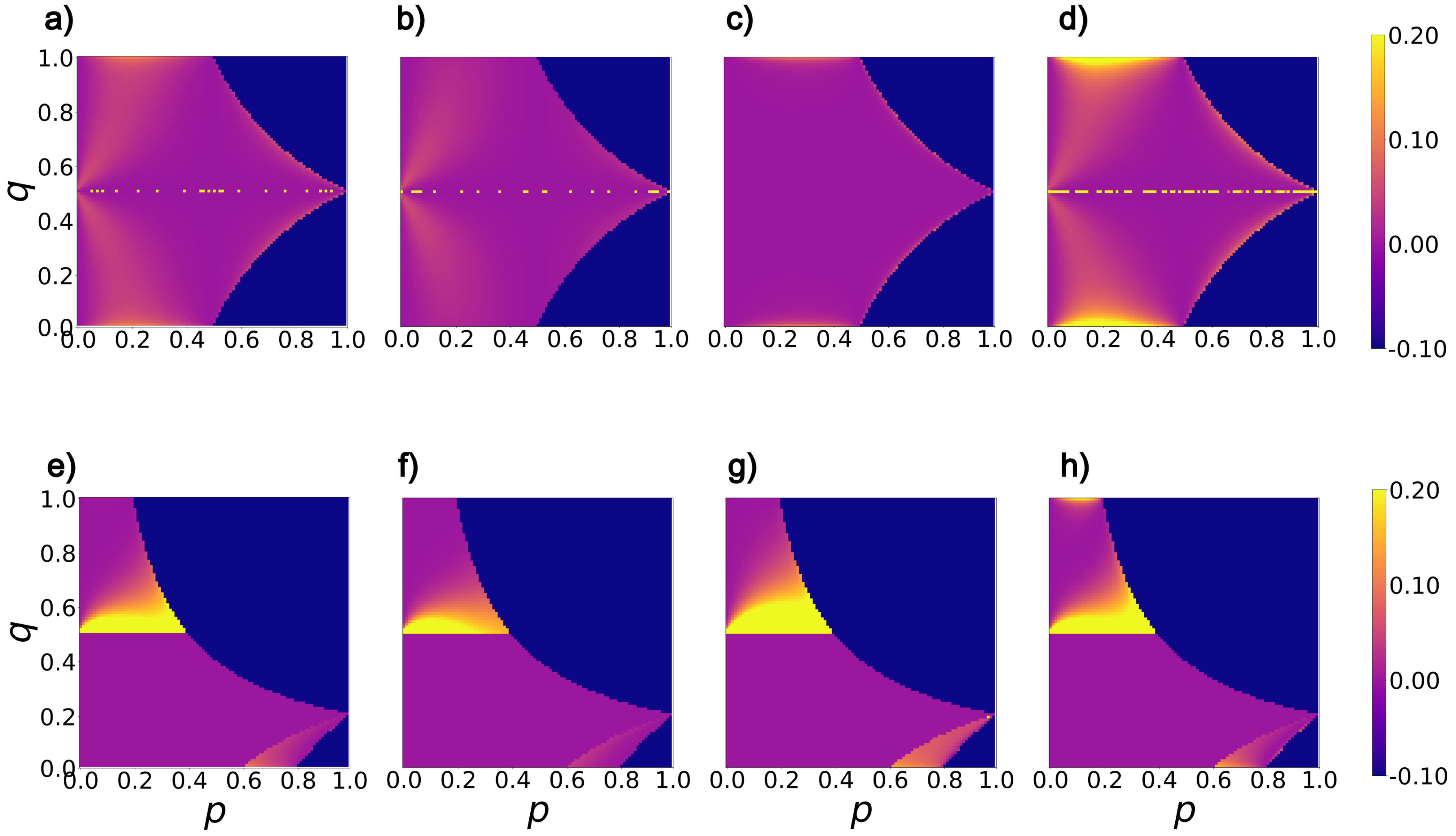
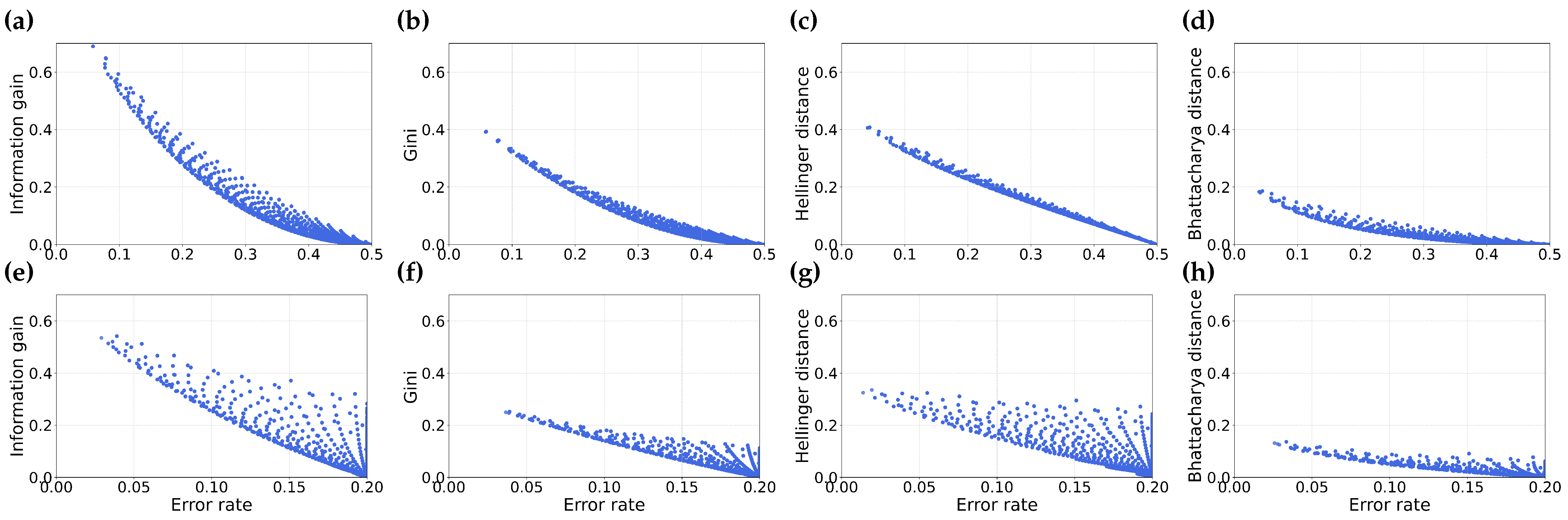
3.2. A Global View of Misordering
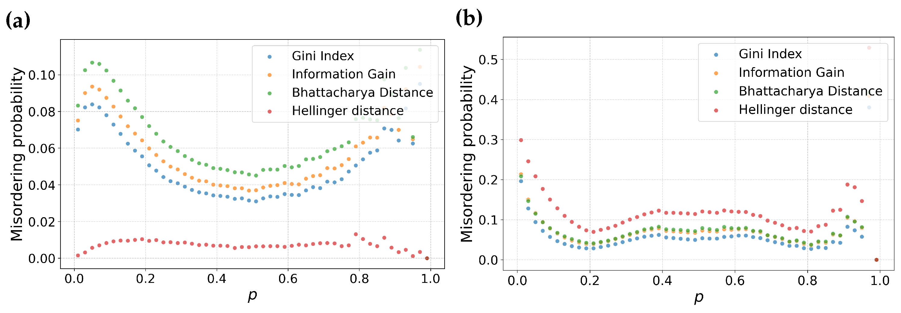
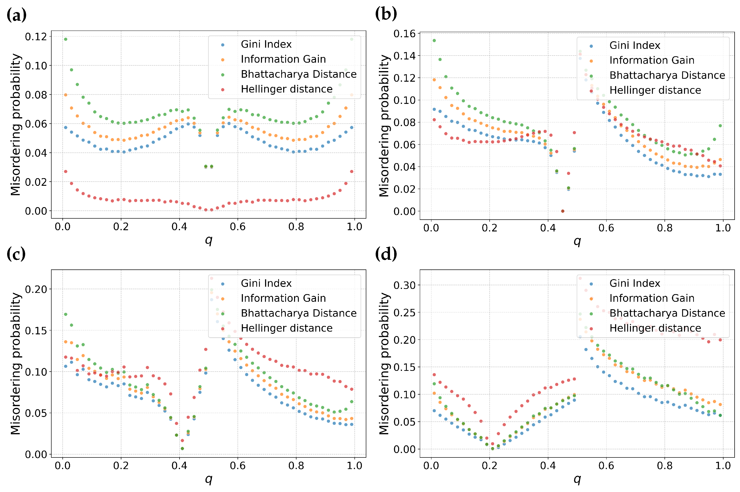
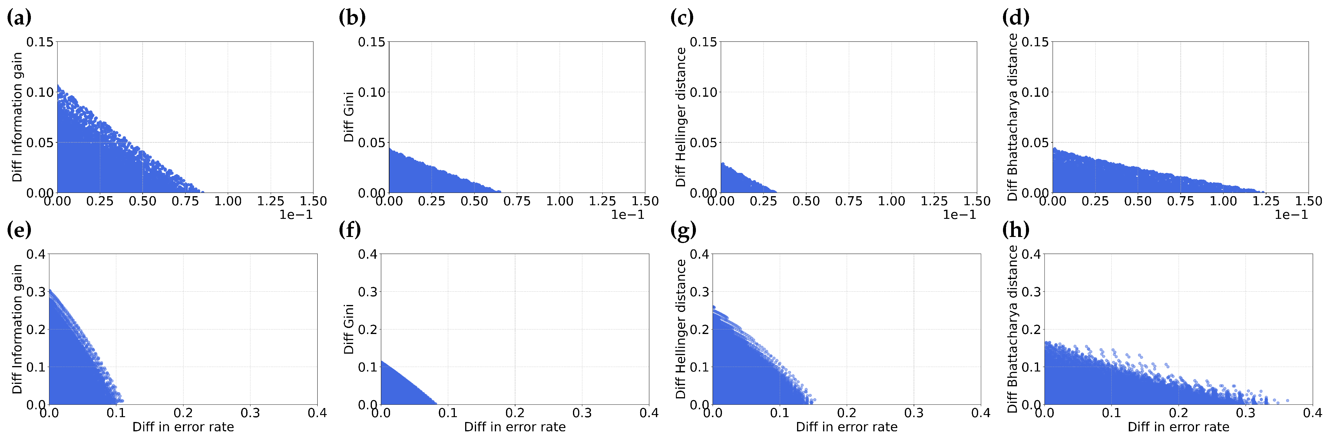
3.3. Is Misordering Confined to Narrow Combinations of Error Rates and Feature Selection Metrics?
3.4. Is Misordering Primarily Due to Numerical Issues?
4. Empirical Comparison and Discussion
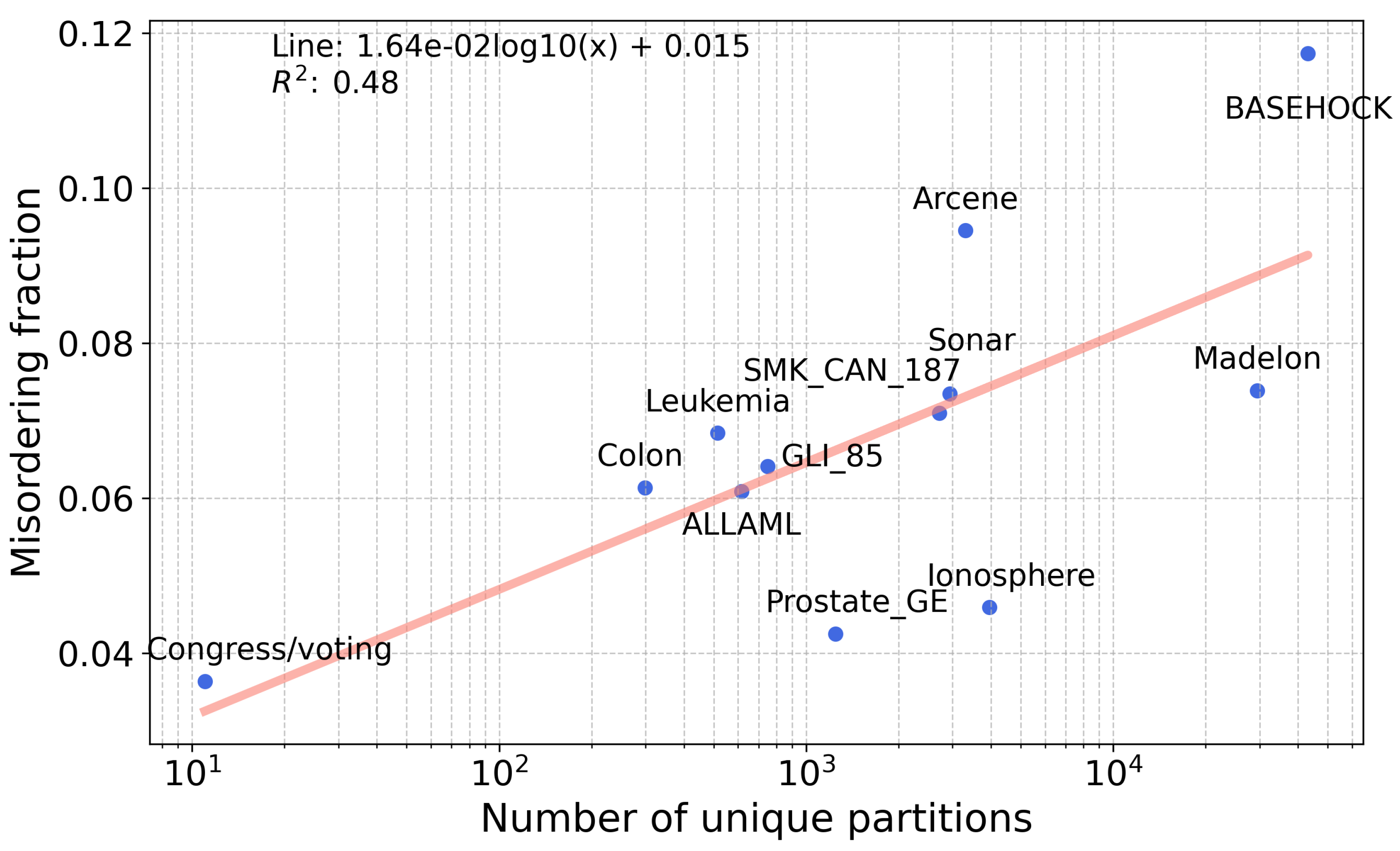
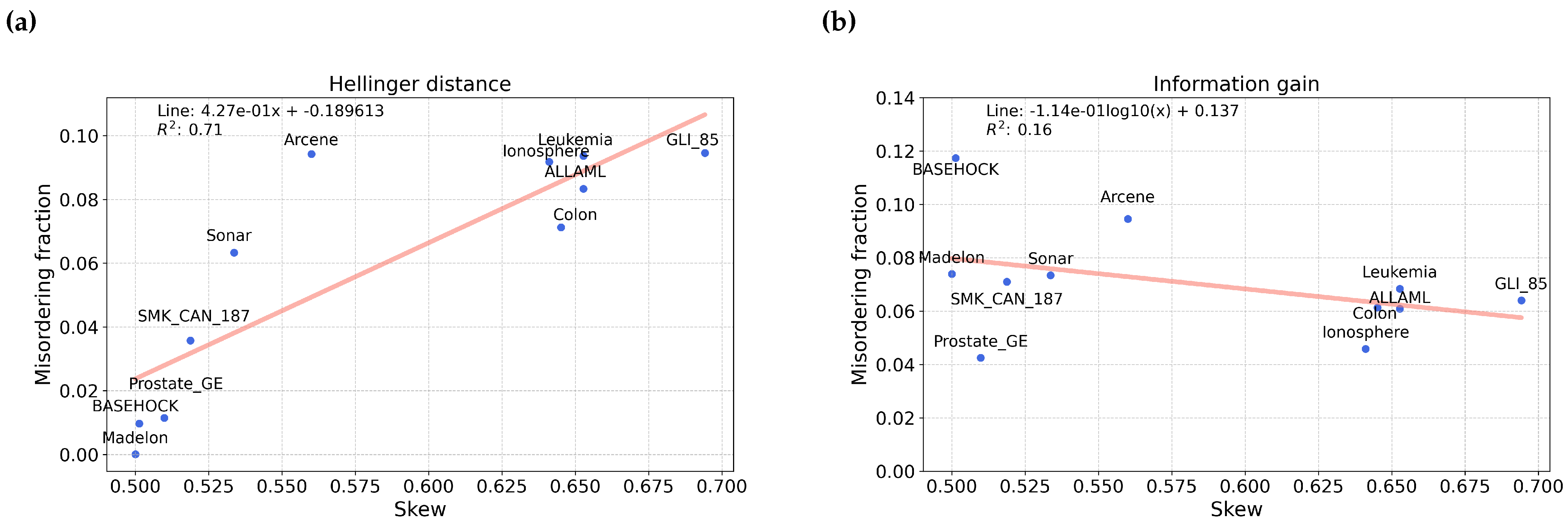
4.1. Misordering on Real-World Datasets
4.2. Potential Misordering in Other Feature Selection Metrics
- Fisher score [24] is a filter method that determines the ratio of the separation between classes and the variance within classes for each feature. The idea is to find a subset of features such that the distances between data points of different classes are as large as possible and the distances between data points of the same class are as small as possible.
- Cons (Consistency Based Filter) [26] is a filter method that measures how much consistency there is in the training data when considering a subset of features [27]. A consistency measure is defined by how often feature values for examples match and the class labels match. A set of features is inconsistent if all of the feature values match, but the class labels differ [28].
- ReliefF [30] randomly samples an example from the data and then determines the two nearest neighbors, where one has the same class label and the other has the opposite class label. These nearest neighbors are determined by using the metric of the p-dimensional Euclidean distance where p is the number of features in the data. The feature values of these neighbors are compared to the example that was sampled and used to update the relevance of each feature to the label. The idea is that a feature that predicts the label well should be able to separate examples with different class labels and predict the same label for examples from the same class [7].
- mRMR [31] chooses features based on the relevance with the target class and also picks features that are minimally redundant with each other. The optimization criteria of minimum redundancy and maximum relevance are based on mutual information [7]. The mutual information between two features represents the dependence between the two variables and thus is used as a measure of redundancy, while the average mutual information over the set of features is used as a measure of relevance. In order to find the minimum redundancy-maximum relevance set of features, these two criteria are optimized simultaneously, which can be done through a variety of heuristics [31].
- FCBF (fast correlation-based filter) [32] first selects a set of features highly correlated with the class label using a metric called Symmetric Uncertainty. Symmetric Uncertainty is the ratio between the information gain and the entropy for two features. Then, three heuristics that keep more relevant features and remove redundant features are applied [7].
4.3. Impact of Misordering on Adaboost
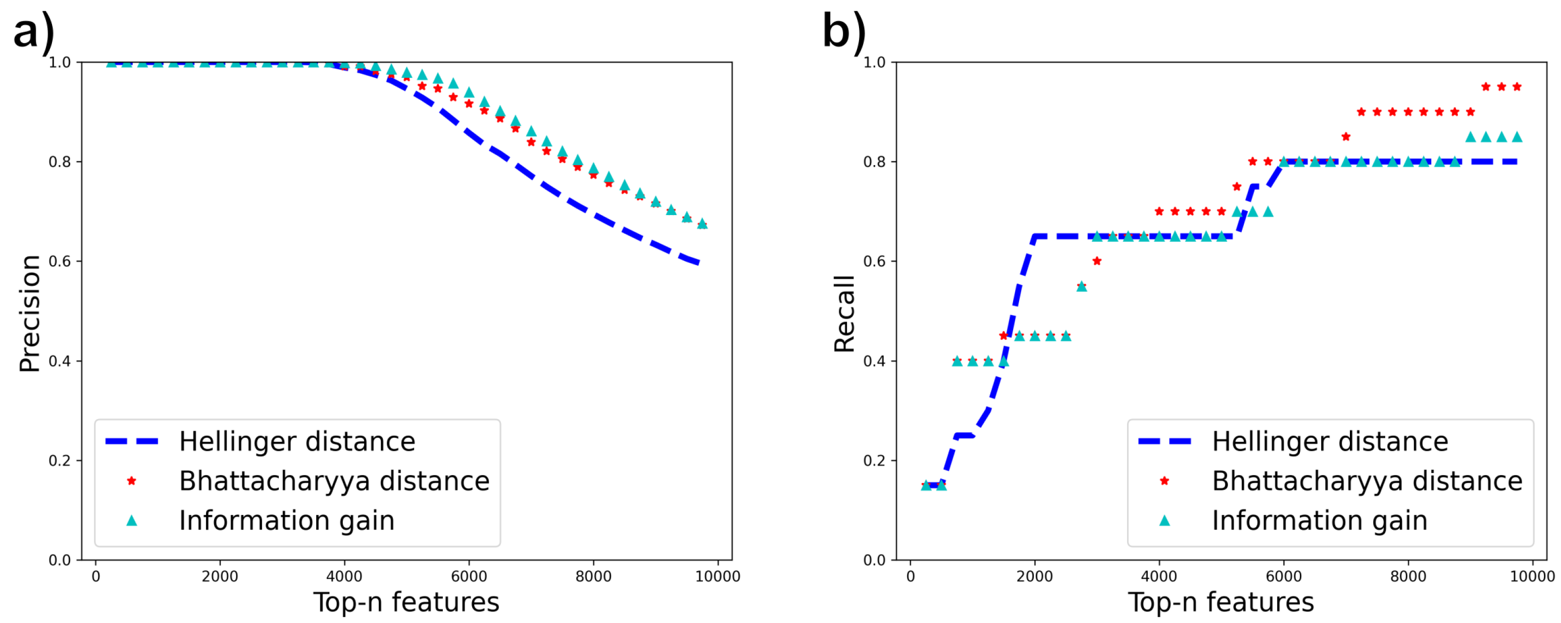
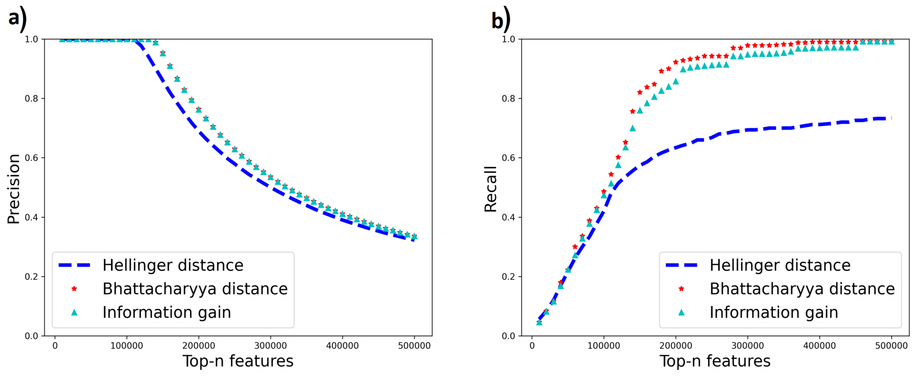
4.4. Impact of Misordering on Feature Selection Precision and Recall
5. Limitations
6. Conclusions
Author Contributions
Funding
Institutional Review Board Statement
Data Availability Statement
Conflicts of Interest
Appendix A
- When a paper lists 2 values of accuracy for the same classifier and dataset, but the only differing factor is the number of features used and the number of features is relatively small, the larger number of features is used. For instance, in Table 10 of [7], the paper reports accuracy values for both using the top 10 features and the top 50 features for using information gain, ReliefF, SVM-RFE, and mRMR. Using the larger number of features is more likely to encompass the target we are trying to capture due to the relatively small number of features used. Note that this point only applies when both information gain and the metric compared to information gain both select the top k values of their metric.
- When information gain and the other metric do not both select the top k values of their metric, the option which allows the 2 metrics to have the closest number of features used in their models is used. For instance, in Table 10 of [7], there are accuracy values for accuracy for both selecting the top 10 features and selecting the top 50 features. However, correlation-based feature selection (CFS) does not select features based on a specific number of top features, so the different datasets have different numbers of features used in the models. Based on Table 9 of [7], the Breast dataset has 130 features selected for CFS, so when comparing information gain and CFS, the value of accuracy using the top 50 features of information gain is compared to the CFS accuracy since 50 is closer to 130 than 10 is to 130.
- When the choice of the cross-validation method is between (1) regular 5-fold cross-validation and (2) distribution-balanced stratified cross-validation(DOB-SCV) with 5 folds, the former is used as it is a more standard option. One example of this occurring is in Table A1 and Table A2 in [7].
- The Sequential Minimal Optimization (SMO) algorithm is an algorithm that solves the quadratic programming problem that comes from training SVMs (Sequential Vector Machines). SMO is used in Table 5.8 of [47], which uses 3 different polynomial kernels (1, 2, and 3). We choose the kernel of 3 since the choice of features should have the biggest effect on this kernel.
- In order to guarantee that each entry in the compared vectors are different enough to guarantee that the entries are independent, similar classifiers cannot be used together with the same dataset. Data that uses logistic regression as the classifier is not used as a linear SVM is essentially the same as logistic regression with a linear kernel. For instance, this occurs in Table 4 of [48] with results for both SVM and logistic regression being reported.
- In some papers, the C4.5 classifier is used with similar datasets. For instance, in [47], the Corral dataset is used. However, [49] uses both the Corral dataset and a modification of the Corral dataset called Corral-100, which adds 93 irrelevant binary features to the Corral dataset. In the correlation calculations, the Corral-100 dataset is used as the irrelevant features add additional selection opinions that help reveal how good each algorithm is. The Led-100 dataset is also used instead of the Led-25 dataset in [49] for the same reasoning.
- When the options for feature dimensions are large (thousands of features), as in Table 1 of [50], the median value is chosen. Once the number of features gets large, the number of features should not make as big of a difference, so the median value is used. If two values of feature dimension are equally close to the median, then the larger value is used.
- When an algorithm uses a population size, such as in an evolutionary algorithm, the option with the larger population size is used as the algorithm will see more options of what features to select. For instance, in Table 1 of [51], the population size of 50 is used.
- Table 13 of [49] uses 2 ranker methods for some feature selection algorithms: (1) selecting the optimal number of features, (2) selecting 20 features. Since the 20 features better encompasses the feature selection problem since the optimal number of features is 2 features.

| Feature Selection Method | List of Papers Used for Calculations |
|---|---|
| Fisher score | [35,52,53] |
| CFS(Correlation Based Feature Selection) | [7,26,27,29,47,48,49] |
| INTERACT | [7,27,49] |
| Cons (Consistency Based Filer) | [26,27,29,48,49] |
| Chi-squared statistic | [29,37,50,53] |
| Relief-F | [7,10,26,27,29,35,47,48,49,53,54] |
| mRMR (Minimum-Redundancy Maximum-Relevance) | [7,10,35,49] |
| FCBF (fast correlation-based filter) | [7,27,29,47] |
| LASSO | [29,35,55] |
| SVM-RFE | [7,29,49] |
References
- Hira, Z.M.; Gillies, D.F. A Review of Feature Selection and Feature Extraction Methods Applied on Microarray Data. Adv. Bioinform. 2015, 2015, 198363. [Google Scholar] [CrossRef] [PubMed]
- Dinga, R.; Penninx, B.W.; Veltman, D.J.; Schmaal, L.; Marquand, A.F. Beyond accuracy: Measures for assessing machine learning models, pitfalls and guidelines. bioRxiv 2019, 743138. [Google Scholar] [CrossRef]
- Guyon, I.; Elisseeff, A. An Introduction to Variable and Feature Selection. J. Mach. Learn. Res. 2003, 3, 1157–1182. [Google Scholar]
- Nguyen, T.; Sanner, S. Algorithms for direct 0–1 loss optimization in binary classification. In Proceedings of the International Conference on Machine Learning, PMLR, Atlanta, GA, USA, 17–19 June 2013; pp. 1085–1093. [Google Scholar]
- Zhou, S.; Pan, L.; Xiu, N.; Qi, H.D. Quadratic convergence of smoothing Newton’s method for 0/1 loss optimization. SIAM J. Optim. 2021, 31, 3184–3211. [Google Scholar] [CrossRef]
- He, X.; Little, M.A. 1248 An efficient, provably exact, practical algorithm for the 0–1 loss linear classification problem. arXiv 2023, arXiv:2306.12344. [Google Scholar]
- Bolón-Canedo, V.; Sánchez-Maroño, N.; Alonso-Betanzos, A.; Benítez, J.; Herrera, F. A review of microarray datasets and applied feature selection methods. Inf. Sci. 2014, 282, 111–135. [Google Scholar] [CrossRef]
- Tangirala, S. Evaluating the Impact of GINI Index and Information Gain on Classification using Decision Tree Classifier Algorithm. Int. J. Adv. Comput. Sci. Appl. 2020, 11, 612–619. [Google Scholar] [CrossRef]
- Mingers, J. An Empirical Comparison of Selection Measures for Decision-Tree Induction; Machine Learning; Springer: Berlin/Heidelberg, Germany, 1989; Volume 3, pp. 319–342. [Google Scholar] [CrossRef]
- Nie, F.; Huang, H.; Cai, X.; Ding, C. Efficient and Robust Feature Selection via Joint ℓ2,1-Norms Minimization. Neural Inf. Process. Syst. 2010, 23. Available online: https://proceedings.neurips.cc/paper_files/paper/2010/file/09c6c3783b4a70054da74f2538ed47c6-Paper.pdf (accessed on 22 November 2023).
- Ferreria, A.J.; Figueuredo, M.A. An unsupervised approach to feature discretization and selection. Pattern Recognit. 2011, 45, 3048–3060. [Google Scholar] [CrossRef]
- Breiman, L.; Friedman, J.; Stone, C.J.; Olshen, R. Classification and Regression Trees; Routledge: London, UK, 1984. [Google Scholar]
- Meyen, S. Relation between Classification Accuracy and Mutual Information in Equally Weighted Classification Tasks. Master’s Thesis, University of Tuebingen, Tubingen, Germany, 2016. [Google Scholar]
- Zhou, Z.H. A brief introduction to weakly supervised learning. Natl. Sci. Rev. 2017, 5, 44–53. [Google Scholar] [CrossRef]
- Quinlan, J.R. C4.5: Programs for Machine Learning; Morgan Kaufmann Publishers Inc.: San Francisco, CA, USA, 1993. [Google Scholar]
- Breiman, L.; Friedman, J.H.; Olshen, R.A.; Stone, C.J. Classification and Regression Trees. Biometrics 1984, 40, 874. [Google Scholar]
- Hellinger, E. Neue begründung der theorie quadratischer formen von unendlichvielen veränderlichen. J. Reine Angew. Math. 1909, 1909, 210–271. [Google Scholar] [CrossRef]
- Bhattacharyya, A. On a measure of divergence between two multinomial populations. Sankhya Indian J. Stat. 1946, 7, 401–406. [Google Scholar]
- Choi, E.; Lee, C. Feature extraction based on the Bhattacharyya distance. Pattern Recognit. 2003, 36, 1703–1709. [Google Scholar] [CrossRef]
- Guyon, I.; Gunn, S.; Ben-Hur, A.; Dror, G. Result Analysis of the NIPS 2003 Feature Selection Challenge with data retrieved from University of California Irvine Machine Learning Repository. 2004. Available online: https://papers.nips.cc/paper/2004/file/5e751896e527c862bf67251a474b3819-Paper.pdf (accessed on 22 November 2023).
- Li, J. Feature Selection Datasets. Data retrieved from Arizona State University. Available online: https://jundongl.github.io/scikit-feature/datasets.html (accessed on 5 October 2023).
- Dua, D.; Graff, C. UCI Machine Learning Repository. 2017. Available online: https://archive.ics.uci.edu/ (accessed on 22 November 2023).
- Grimaldi, M.; Cunningham, P.; Kokaram, A. An Evaluation of Alternative Feature Selection Strategies and Ensemble Techniques for Classifying Music. Workshop on Multimedia Discovery and Mining. 2003. Available online: https://citeseerx.ist.psu.edu/document?repid=rep1&type=pdf&doi=22a1a59619809e8ecf7ff051ed262bea0f835f92#page=44 (accessed on 22 November 2023).
- Duda, R.O.; Hart, P.E.; Stork, D.G. Pattern Classification; Wiley-Interscience Publication: Hoboken, NJ, USA, 2000. [Google Scholar]
- Hall, M.A. Correlation-Based Feature Selection for Machine Learning. Ph.D. Thesis, The University of Waikato, Hamilton, New Zealand, 1999. Available online: https://www.cs.waikato.ac.nz/~mhall/thesis.pdf (accessed on 5 October 2023).
- Hall, M.A.; Holmes, G. Benchmarking Attribute Selection Techniques for Discrete Class Data Mining. IEEE Trans. Knowl. Data Eng. 2003, 15, 1437–1447. [Google Scholar] [CrossRef]
- Bolon-Canedo, V.; Sanchez-Marono, N.; Alonso-Betanzos, A. An ensemble of filters and classifiers for microarray data classification. Pattern Recognit. 2012, 45, 531–539. [Google Scholar] [CrossRef]
- Dash, M.; Liu, H. Consistency-based search in feature selection. Artif. Intell. 2003, 151, 155–176. [Google Scholar] [CrossRef]
- Singh, N.; Singh, P. A hybrid ensemble-filter wrapper feature selection approach for medical data classification. Chemom. Intell. Lab. Syst. 2021, 217, 104396. [Google Scholar] [CrossRef]
- Kononenko, I. Estimating attributes: Analysis and extensions of RELIEF. In European Conference on Machine Learning; Springer: Berlin/Heidelberg, Germany, 1994. [Google Scholar]
- Ding, C.; Peng, H. Minimum Redundancy Feature Selection from Microarray Gene Expression Data. J. Bioinform. Comput. Biol. 2005, 3, 185–205. [Google Scholar] [CrossRef]
- Yu, L.; Liu, H. Feature Selection for High-Dimensional Data: A Fast Correlation-Based Filter Solution. In Proceedings of the Twentieth International Conference on Machine Learning, Washington, DC, USA, 21–24 August 2003. [Google Scholar]
- Zhao, Z.; Liu, H. Searching for Interacting Features. In Proceedings of the 20th International Joint Conference on Artificial Intelligence, Hyderabad, India, 6–12 January 2007. [Google Scholar]
- Tibshirani, R. Regression Shrinkage and Selection via the Lasso. J. R. Stat. Soc. 1996, 58, 267–288. [Google Scholar] [CrossRef]
- Nardone, D.; Ciaramella, A.; Staiano, A. A Sparse-Modeling Based Approach for Class Specific Feature Selection. PeerJ Comput. Sci. 2019, 5, e237. [Google Scholar] [CrossRef] [PubMed]
- Guyon, I.; Weston, J.; Barnhill, S.; Vapnik, V. Gene Selection for Cancer Classification using Support Vector Machines. Mach. Learn. 2002, 46, 389–422. [Google Scholar] [CrossRef]
- Manek, A.S.; Shenoy, P.D.; Mohan, M.C.; R, V.K. Aspect term extraction for sentiment analysis in large movie reviews using Gini Index feature selection method and SVM classifier. World Wide Web 2016, 20, 135–154. [Google Scholar] [CrossRef]
- Epstein, E. The Relationship between Common Feature Selection Metrics and Accuracy. Master’s Thesis, Case Western Reserve University, Cleveland, OH, USA, 2022. [Google Scholar]
- Pearson, K. Notes on the History of Correlation. Biometrika 1920, 13, 25–45. [Google Scholar] [CrossRef]
- Freund, Y.; Schapire, R.E. A decision-theoretic generalization of on-line learning and an application to boosting. J. Comput. Syst. Sci. 1997, 55, 119–139. [Google Scholar] [CrossRef]
- Schapire, R.E. The Design and Analysis of Efficient Learning Algorithms. Ph.D. Thesis, MIT Press , Cambridge, MA, USA, 1992. [Google Scholar]
- Burl, M.C.; Asker, L.; Smyth, P.; Fayyad, U.; Perona, P.; Crumpler, L.; Aubele, J. Learning to recognize volcanoes on Venus. Mach. Learn. 1998, 30, 165–194. [Google Scholar] [CrossRef]
- Ouyang, T.; Ray, S.; Rabinovich, M.; Allman, M. Can network characteristics detect spam effectively in a stand-alone enterprise? In Proceedings of the Passive and Active Measurement: 12th International Conference, PAM 2011, Atlanta, GA, USA, 20–22 March 2011; Proceedings 12. Springer: Berlin/Heidelberg, Germany, 2011; pp. 92–101. [Google Scholar]
- Guyon, I. Madelon. UCI Machine Learning Repository. 2008. Available online: https://archive.ics.uci.edu/dataset/171/madelon (accessed on 22 November 2023).
- Guyon, I.; Gunn, S.; Ben-Hur, A.; Dror, G. Gisette. UCI Machine Learning Repository. 2008. Available online: https://archive.ics.uci.edu/dataset/170/gisette (accessed on 22 November 2023).
- Kursa, M.B.; Rudnicki, W.R. Feature Selection with the Boruta Package. J. Stat. Softw. 2010, 36, 1–13. [Google Scholar] [CrossRef]
- Sui, B. Information Gain Feature Selection Based On Feature Interactions. Master’s Thesis, University of Houston, Houston, TX, USA, 2013. [Google Scholar]
- Koprinska, I. Feature Selection for Brain-Computer Interfaces. PAKDD 2009 International Workshops. 2009. Available online: https://link.springer.com/content/pdf/10.1007/978-3-642-14640-4.pdf (accessed on 1 October 2023).
- Bolón-Canedo, V.; Sánchez-Maroño, N.; Alonso-Betanzos, A. A Review of Feature Selection Methods on Synthetic Data. Knowl. Inf. Syst. 2013, 34, 483–519. [Google Scholar] [CrossRef]
- Wu, L.; Wang, Y.; Zhang, S.; Zhang, Y. Fusing Gini Index and Term Frequency for Text Feature Selection. In Proceedings of the 2017 IEEE Third International Conference on Multimedia Big Data, Laguna Hills, CA, USA, 19–21 April 2017. [Google Scholar]
- Jirapech-Umpai, T.; Aitken, S. Feature selection and classification for microarray data analysis: Evolutionary methods for identifying predictive genes. BMC Bioinform. 2005, 6, 148. [Google Scholar] [CrossRef]
- Masoudi-Sobhanzadeh, Y.; Motieghader, H.; Masoudi-Nejad, A. FeatureSelect: A software for feature selection based on machine. learning approaches. BMC Bioinform. 2019, 20, 170. [Google Scholar] [CrossRef]
- Phuong, H.T.M.; Hanh, L.T.M.; Binh, N.T. A Comparative Analysis of Filter-Based Feature Selection Methods for Software Fault Prediction. Res. Dev. Inf. Commun. Technol. 2021. [Google Scholar] [CrossRef]
- Taheri, N.; Nezamabadi-pour, H. A hybrid feature selection method for high-dimensional data. In Proceedings of the 4th International Conference on Computer and Knowledge Engineering, Mashhad, Iran, 29–30 October 2014. [Google Scholar]
- Bi, X.; Liu, J.G.; Cao, Y.S. Classification of Low-grade and High-grade Glioma using Multiparametric Radiomics Model. In Proceedings of the IEEE 3rd Information Technology, Networking, Electronic and Automation Control Conference (ITNEC 2019), Chengdu, China, 15–17 March 2019. [Google Scholar]


| Sharp Teeth? | Has Fur? | Lazy? | Loud? | Is Lion? (Label) |
|---|---|---|---|---|
| No | No | Yes | No | Yes |
| No | Yes | No | No | No |
| Yes | No | Yes | No | No |
| Yes | Yes | Yes | No | Yes |
| Yes | Yes | No | No | No |
| Yes | No | No | No | No |
| Yes | Yes | Yes | No | Yes |
| Yes | Yes | No | No | Yes |
| Yes | Yes | No | Yes | Yes |
| Dataset | Percent Majority Class | Number of Examples | Number of Features | Number of Unique Feature Splits | Feature Type |
|---|---|---|---|---|---|
| Gisette | 0.500 | 7000 | 5000 | 478,699 | Continuous |
| Madelon | 0.500 | 2600 | 500 | 29,490 | Continuous |
| BASEHOCK | 0.501 | 1993 | 4862 | 43,109 | Discrete |
| Prostate_GE | 0.510 | 102 | 5966 | 1245 | Continuous |
| SMK_CAN_187 | 0.519 | 187 | 19,993 | 2715 | Continuous |
| Sonar | 0.534 | 208 | 60 | 2941 | Continuous |
| Arcene | 0.560 | 200 | 10,000 | 3308 | Continuous |
| Congressional Voting | 0.614 | 435 | 16 | 11 | Binary |
| Ionosphere | 0.641 | 351 | 34 | 3958 | Continuous |
| Colon | 0.645 | 62 | 2000 | 299 | Discrete |
| ALLAML | 0.653 | 72 | 7129 | 615 | Continuous |
| Leukemia | 0.653 | 72 | 7070 | 515 | Discrete |
| GLI_85 | 0.694 | 85 | 22,283 | 749 | Continuous |
| Dataset | Percent Majority Class | Information Gain | Gain Ratio | Gini Index | Hellinger Distance | Bhattacharyya Distance |
|---|---|---|---|---|---|---|
| Gisette | 0.500 | 0.0612 | 0.116 | 0.0572 | 0.0024 | 0.0562 |
| Madelon | 0.500 | 0.0739 | 0.143 | 0.0683 | 0.0001 | 0.0455 |
| BASEHOCK | 0.501 | 0.117 | 0.209 | 0.113 | 0.0097 | 0.1122 |
| Prostate_GE | 0.510 | 0.0425 | 0.0837 | 0.0325 | 0.0115 | 0.0593 |
| SMK_CAN_187 | 0.519 | 0.0710 | 0.127 | 0.0629 | 0.0357 | 0.0805 |
| Sonar | 0.534 | 0.0734 | 0.113 | 0.0686 | 0.0633 | 0.0775 |
| Arcene | 0.560 | 0.0945 | 0.124 | 0.0851 | 0.0943 | 0.1037 |
| Congressional Voting | 0.614 | 0.0364 | 0.0182 | 0.0364 | 0.0364 | 0.0545 |
| Ionosphere | 0.641 | 0.0459 | 0.0263 | 0.0433 | 0.0918 | 0.0454 |
| Colon | 0.645 | 0.0614 | 0.0603 | 0.0490 | 0.0713 | 0.0716 |
| ALLAML | 0.653 | 0.0609 | 0.0564 | 0.0444 | 0.0833 | 0.0738 |
| Leukemia | 0.653 | 0.0684 | 0.0631 | 0.0551 | 0.0936 | 0.0793 |
| GLI_85 | 0.694 | 0.0641 | 0.0480 | 0.0489 | 0.0946 | 0.0745 |
| Feature Selection Method | Pearson’s Coef. | p-Value | # Data Points |
|---|---|---|---|
| Fisher score | 0.961 | 22 | |
| CFS (Correlation Based Feature Selection) | 0.929 | 213 | |
| INTERACT | 0.913 | 92 | |
| Cons (Consistency Based Filter) | 0.912 | 187 | |
| Chi-squared statistic | 0.899 | 96 | |
| Relief-F | 0.861 | 240 | |
| mRMR | 0.851 | 71 | |
| FCBF (fast correlation-based filter) | 0.836 | 134 | |
| LASSO | 0.726 | 90 | |
| SVM-RFE | 0.660 | 142 |
| Dataset | Iteration | IG/Train | Err/Train | IG/Test | Err/Test |
|---|---|---|---|---|---|
| Volcanoes [42] | 1 | 0.841 | 0.841 | 0.029 | 0.029 |
| 2 | 0.841 | 0.841 | 0.029 | 0.029 | |
| 3 | 0.841 | 0.841 | 0.029 | 0.029 | |
| 4 | 0.845 | 0.855 | 0.166 | 0.126 | |
| 5 | 0.845 | 0.855 | 0.166 | 0.126 | |
| 6 | 0.845 | 0.842 | 0.164 | 0.235 | |
| 7 | 0.839 | 0.866 | 0.211 | 0.161 | |
| 8 | 0.846 | 0.867 | 0.155 | 0.191 | |
| 9 | 0.840 | 0.864 | 0.211 | 0.112 | |
| 10 | 0.846 | 0.871 | 0.155 | 0.197 | |
| Spam [43] | 1 | 0.663 | 0.712 | 0.668 | 0.707 |
| 2 | 0.663 | 0.712 | 0.668 | 0.707 | |
| 3 | 0.663 | 0.712 | 0.668 | 0.707 | |
| 4 | 0.675 | 0.706 | 0.677 | 0.714 | |
| 5 | 0.721 | 0.715 | 0.715 | 0.716 | |
| 6 | 0.721 | 0.717 | 0.715 | 0.718 | |
| 7 | 0.721 | 0.719 | 0.715 | 0.713 | |
| 8 | 0.711 | 0.722 | 0.706 | 0.720 | |
| 9 | 0.719 | 0.720 | 0.714 | 0.713 | |
| 10 | 0.719 | 0.723 | 0.714 | 0.721 | |
| Ionosphere [22] | 1 | 0.864 | 0.864 | 0.700 | 0.700 |
| 2 | 0.864 | 0.864 | 0.700 | 0.700 | |
| 3 | 0.914 | 0.907 | 0.886 | 0.771 | |
| 4 | 0.893 | 0.907 | 0.771 | 0.714 | |
| 5 | 0.893 | 0.904 | 0.771 | 0.743 | |
| 6 | 0.896 | 0.929 | 0.771 | 0.786 | |
| 7 | 0.925 | 0.907 | 0.800 | 0.786 | |
| 8 | 0.896 | 0.932 | 0.771 | 0.800 | |
| 9 | 0.943 | 0.932 | 0.800 | 0.786 | |
| 10 | 0.911 | 0.946 | 0.771 | 0.857 | |
| Hepatitis [22] | 1 | 0.889 | 0.889 | 0.875 | 0.875 |
| 2 | 0.889 | 0.889 | 0.875 | 0.875 | |
| 3 | 0.889 | 0.905 | 0.875 | 1.000 | |
| 4 | 0.905 | 0.921 | 1.000 | 1.000 | |
| 5 | 0.857 | 0.952 | 1.000 | 1.000 | |
| 6 | 0.952 | 0.968 | 1.000 | 1.000 | |
| 7 | 0.984 | 0.968 | 1.000 | 1.000 | |
| 8 | 0.968 | 0.968 | 1.000 | 1.000 | |
| 9 | 0.984 | 0.984 | 1.000 | 1.000 | |
| 10 | 0.952 | 0.984 | 1.000 | 1.000 | |
| German [22] | 1 | 0.700 | 0.715 | 0.680 | 0.725 |
| 2 | 0.700 | 0.715 | 0.680 | 0.725 | |
| 3 | 0.723 | 0.730 | 0.735 | 0.710 | |
| 4 | 0.717 | 0.741 | 0.715 | 0.740 | |
| 5 | 0.715 | 0.742 | 0.715 | 0.745 | |
| 6 | 0.715 | 0.750 | 0.715 | 0.740 | |
| 7 | 0.725 | 0.751 | 0.735 | 0.725 | |
| 8 | 0.736 | 0.761 | 0.715 | 0.730 | |
| 9 | 0.757 | 0.770 | 0.715 | 0.740 | |
| 10 | 0.762 | 0.760 | 0.715 | 0.730 |
| Dataset | Information Gain | Hellinger Distance | Bhattacharyya Distance |
|---|---|---|---|
| Madelon | 0.0739 | 0.0001 | 0.045 |
| Gisette-small | 0.0534 | 0.0007 | 0.034 |
Disclaimer/Publisher’s Note: The statements, opinions and data contained in all publications are solely those of the individual author(s) and contributor(s) and not of MDPI and/or the editor(s). MDPI and/or the editor(s) disclaim responsibility for any injury to people or property resulting from any ideas, methods, instructions or products referred to in the content. |
© 2023 by the authors. Licensee MDPI, Basel, Switzerland. This article is an open access article distributed under the terms and conditions of the Creative Commons Attribution (CC BY) license (https://creativecommons.org/licenses/by/4.0/).
Share and Cite
Epstein, E.; Nallapareddy, N.; Ray, S. On the Relationship between Feature Selection Metrics and Accuracy. Entropy 2023, 25, 1646. https://doi.org/10.3390/e25121646
Epstein E, Nallapareddy N, Ray S. On the Relationship between Feature Selection Metrics and Accuracy. Entropy. 2023; 25(12):1646. https://doi.org/10.3390/e25121646
Chicago/Turabian StyleEpstein, Elise, Naren Nallapareddy, and Soumya Ray. 2023. "On the Relationship between Feature Selection Metrics and Accuracy" Entropy 25, no. 12: 1646. https://doi.org/10.3390/e25121646
APA StyleEpstein, E., Nallapareddy, N., & Ray, S. (2023). On the Relationship between Feature Selection Metrics and Accuracy. Entropy, 25(12), 1646. https://doi.org/10.3390/e25121646