1. Introduction
The classical Shannon entropy (see Shannon [
1]) associated with a random variable (RV)
X has a crucial role in many branches of science to measure the uncertainty contained in
Throughout the paper,
X denotes a non-negative RV with an absolutely continuous cumulative distribution function (CDF) with corresponding probability density function (PDF)
The Shannon differential entropy is
Possible alternative measures of information have been introduced in the literature.
The cumulative residual entropy (CRE) initiated by Rao et al. [
2] as a counterpart to (
1), obtained by substituting the survival function (SF)
in place of the PDF
as
where
is the cumulative the hazard rate (HR) function and
is the HR function. Dynamic versions of the CRE were considered in Asadi and Zohrevand [
3] and also in Navarro et al. [
4] where the CRE of the residual lifetime
was measured as
For related results, one can see Baratpour [
5], Baratpour and Habibi Rad [
6] and also Toomaj et al. [
7] and the references therein. In a recent work by Di Crescenzo et al. [
8], the CRE measure was extended to FGCRE as
where
. The notation
is used across the paper. Note that
The properties of fractional cumulative entropy, such as its alteration under linear transformations, its bounds, its connection to stochastic orders along with its empirical estimation, and various relations to other functions have been argued and discussed by Xiong et al. [
9]. We note that, as pointed out by [
8], if
is a positive integer, say,
then
is identical to the generalized cumulative residual entropy (GCRE) introduced by Psarrakos and Navarro [
10]. It is noticeable that
is considered a dispersion measure. The measure is also connected to the relevance transformation and interepoch intervals of a nonhomogeneous Poisson process (see, e.g., Toomaj and Di Crescenzo [
11]). This paper aims to continue this line of research. In this context, we present new findings on the FGRCE and its dynamic version. The FGCRE is in particular a suitable quantity to be applied in the proportional HR model.
The subsequent materials of this article are organized in the following order. In
Section 2, we first give an overview of the concept of generalized cumulative residual entropy and present a similar representation for fractional generalized residual cumulative entropy. We then give some expressions for the FGCRE, one of which is related to the MRL function. We also consider the connection of the FGCRE with the excess wealth order and the Bayesian risk of the FGCRE. A normalized version of the FGCRE is given and its connection with the Lorenz curve order is studied.
Section 3 examines some bounds and stochastic ordering properties of FGCRE. In
Section 4, properties of the dynamic FGCRE are discussed.
The reader can be referred to [
12] for the definitions of stochastic orders
and
and for the definitions of (increasing) decreasing MRL (IMRL(DMRL)), (decreasing) increasing failure rate (DFR (IFR)) and new better (worse) than used in expectation (NBUE (NWUE)) classes.
2. Basic Properties
As mentioned earlier, the FGCRE in (
4) reduces to the GCRE when
In this case,
for all
. As pointed out by Psarrakos and Navarro [
10], the GCRE fulfills the following property:
where
and
denotes the epoch times of a Poisson process which is nonhomogeneous having intensity function
. Note that
and
X are equally distributed. Signifying by
the SF of
one has (see Baxter [
13])
and the PDF of
is
In the following, we show that the same results can be obtained for the FGCRE. It is worth noting that our results are extensions of the results obtained using the GCRE. To this end, we define the RV
with the PDF as
for all
where
is defined in (
3). Denoting by
the SF of
it can be represented as
where
is increasing in
t for all
If
is an integer, say,
then (
9) reduces to (
8). Notice that from (
4), the FGCRE can be rewritten as
for all
From (
9), the ratio
is increasing in
t and, therefore,
for any
In particular, this implies that
. That is,
for all
. Hence, if
X is IFR (DFR), then, from (
10) and Equation (1.A.7) in [
12], we have
for all
. In
Table 1, we give FGCREs for a number of distributions.
Now, we obtain an analogue representation for the FGCRE which is a generalization of relation (
6) with FGCRE in place of GCRE.
Proposition 1. Let X have FGCRE Then, for all Proof. Recalling (
4) and integrating by parts, we obtain
where the last equality is obtained by recalling (
9) and using
. □
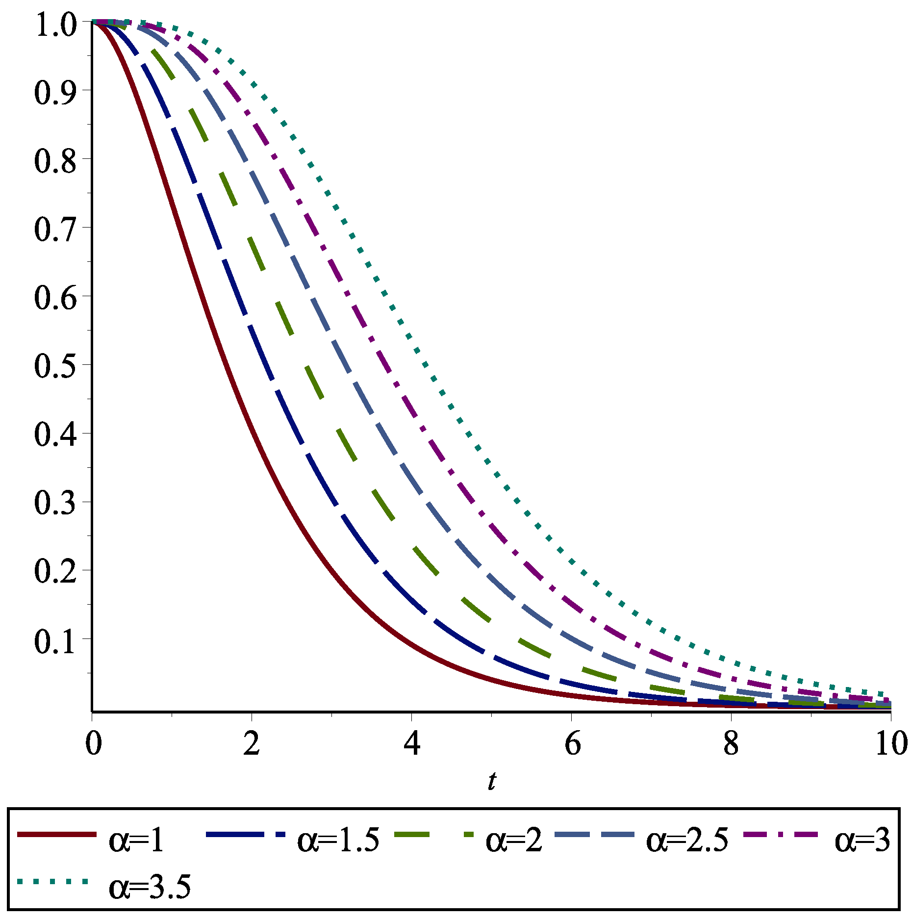
Note that
is the areas surrounded between
and
for all
. In particular,
is the area under
. In
Figure 1, we depict these areas for the exponential distribution and various values of
.
Theorem 1. (i) If, for some then for all .
(ii) If, for some then for all .
Proof. (i) It is not difficult to see whether for each
and
one can obtain
By taking
for
we obtain
Thus, one concludes
where the third inequality is obtained by virtue of the Markov inequality. The last expression is finite if
and this completes the proof. In the case when
the results apply to
□
Note that
does not guarantee equality in the distributions of
X and
Y, but the converse holds. If
where
is strictly increasing and differentiable, then
for all
Below, the connection between the FGCRE and the cumulative HR function of
X given by (
3) is realized.
Theorem 2. Let X fulfill for all . Then,where Proof. From (
4) and also by applying Fubini’s theorem,
which immediately validates (
15) by using (
16). □
We note that
in (
16) is increasing and convex in
This immediately generates the following property.
Theorem 3. Let X have a finite mean μ. Then,for all Another useful application of Theorem 2 is given here.
Theorem 4. If X and Y are non-negative RVs in the way , it holds thatwhere the function is given in (16). In particular, implies Proof. Since
is a convex function and also since it is an increasing function for all
, thus (see Theorem 4.A.8 in [
12]),
. Now, using relation 4.A.2 in [
12], we derive
. □
Clearly,
is increasing and also convex and
Hence, for the RVs
X and
Y satisfying
we obtain that
for all
This relation is immediately obtained from Theorem 2 and Shaked and Shantikumar [
12] (see page 24). It is worth pointing out that Equation (
17) leads us to define the normalized FGCRE by
Under the condition
Equation (
17) can be rewritten as
for
Moreover, if
X is a non-negative RV having IFR (DFR) property, from relation (
11), one can conclude that
From this, we derive that
For
, the normalized cumulative residual entropy
is generated (see Rao [
2]). This is an analogue for the coefficient of variation of an RV. In
Table 2, we give the normalized FGCREs for some distributions.
To continue our results, consider the following observation.
Theorem 5. Let for all . Thenwhere Proof. Recalling Proposition 1 and the change of
, we have
where
for all
In (
20), let
and
Then
and
Integrating by parts gives
and this gives the proof. □
When
the De Vergottini index of inequality of an income distribution
X is reached, given by
(see Rao et al. [
2] for more details). The index (
19) belongs to the class of linear measures of income inequality defined by Mehran [
14]. It can be obtained by weighting the Lorenz differences
together with the income distribution.
Theorem 6. Let and be non-negative RVs with survival functions and respectively. If then for all
Proof. Assumption
implies that
due to Theorem 3.A.10 in [
12]. From relation (
19), we obtain
where the inequality is obtained by noting that
is a non-negative function for all
The result is obtained by reversing. □
The Bayes Risk of MRL
The PDF of
is given by
for
Denote by
the MRL function of
X. In the decision theoretic framework, the MRL function is the optimal prediction of
under the conditional quadratic loss function
as the mean of the PDF
In other words, we have
for all
The function
is a local risk measure, given the value the threshold
t takes. Its global risk of the MRL function of
X is the Bayes risk
where
denotes the average based on the prior PDF for the threshold
t (see Ardakani et al. [
15] and Asadi et al. [
16] for more details). The following theorem provides expressions for
under different priors.
Theorem 7. Let X have the MRL function and let Then, the Bayes risk of is given by the FGCRE functional of the baseline CDF, i.e., Proof. By substituting
for all
we have
The second equality follows by observing that
and the proof is completed. □
From Theorem 7, it is obvious that
for all
We point out that the representation in (
23) is very useful since in many statistical models one may gather information about the behaviour of MRL. The following example illustrates a well-known situation in this context.
Example 1. Let us suppose , , with , and Oakes and Dasu [17] observed that the corresponding SF is It is a well-known property for the generalized Pareto distribution (GPD) as a fundamental aspect of this family of distributions. The exponential distribution is reached whenever , the Pareto distribution is resulted for and the power distribution is achieved for Hence, from (23), the FGCRE of the GPD distribution is derived aswhere the identity for all , has been applied. The Bayes risk of under the prior is given by for all
4. Dynamic FGRCE
The study of the times for events or the age of units is of interest in many fields. The FGCRE of
is
for all
. It is clear that
. The HR of
is
for
Hence, if
X is IFR(DFR), then
is also IFR(DFR) and, therefore,
for all
. On the other hand, by using the generalized binomial expansion, for all
,
In analogy with Theorem 1, the next result is procured:
The dynamic version of identity (
22) follows from the following identity,
which is the PDF of the conditional RV
,
. This is the generalization of expression given in (33) of Toomaj and Di Crescenzo [
11] when
is a positive integer. The result in Theorem 10 of Toomaj and Di Crescenzo [
11] is generalized as follows:
Theorem 15. In the setting of Theorem 7, for non-negative α and t, Theorem 16. For any and for all it holds that Proof. Let us denote
. We obtain
From (
32), one can easily obtain
and
so that
The result now follows from (
31). □
For Theorem 16 is reduced to the next achievement:
In a similar manner as in Theorem 9, the following bounds for the dynamic measure (
4) are derived for
:
The following theorem with the same arguments as in the proof of Theorem 10 gives the dynamic version of the FGCRE.
Theorem 17. For X with a finite MRL function and finite for all we have:
- (i)
in which is as before. denotes the dynamic Shannon entropy introduced in [20]. - (ii)
Moreover, following the proof of Theorem 11, a couple of upper bounds for the dynamic FGCRE are acquired. The definition and properties of the variance residual lifetime (VRL) function in the context of lifetime data analysis have been studied in Gupta [
21], Gupta et al. [
22] and Gupta and Kirmani [
23], among others.
Theorem 18. Let X have a VRL function and finite dynamic FGCRE for all Then,
- (i)
for all
- (ii)
, where for and for and
Now, we give an expression for the derivative of
Proof. By differentiating, we obtain
Applying
and using again (
33),
that is, (
35) holds. □
The preceding theorem can be applied to present the following theorem:
Theorem 20. If X is IFR (DFR), then is decreasing (increasing) for all
Proof. The result is immediate for
since
and since the IFR (DFR) property is stronger than the DMRL (IMRL) property. For all
using relation (
30), we have
which validates the theorem by using Theorem 19. □
Let us define a new aging notion based on the FGCRE.
Definition 1. The RV X has an increasing (decreasing) dynamic FGCRE of order α, and denote it by if is increasing (decreasing) in
We note that the and classes correspond to the IMRL (increasing MRL) and DMRL (decreasing MRL) classes, respectively. In the next theorem, we prove is a subclass of for all .
Lemma 2. Let for a fixed Then Under the assumptions of Lemma 2, is an absolutely continuous function. Furthermore, for then is also absolutely continuous under the hypothesis that Moreover, we have the following result.
Theorem 21. If X is then X is for all .
Proof. Suppose that
X is
. Then, by using (
36), we obtain
for all
Then (
35) yields
and
X is
. The proof is similarly carried out when
X is
. □
From Theorem 21, we can conclude that
and
for all
An immediate consequence of the above relation is that
for all
We remark that Navarro et al. (2010) provided some examples showing that an RV
X is
but it is not IMRL (DMRL). However, Navarro and Psarrakos [
24] by some counterexamples showed that
X is neither IMRL (DMRL) nor
but it is included in the class
when
is an integer value. Hence, the result holds for all
This section is closed by introducing the dynamic normalized version of the FGCRE as follows:
for all
Theorem 22. Let X have a finite normalized FGCRE If X is IMRL (DMRL), then for all
Proof. Since
X is IMRL (DMRL) based on the assumption, we have
Therefore, from Equations (
33) and (
37), we obtain
from which we have the result. □
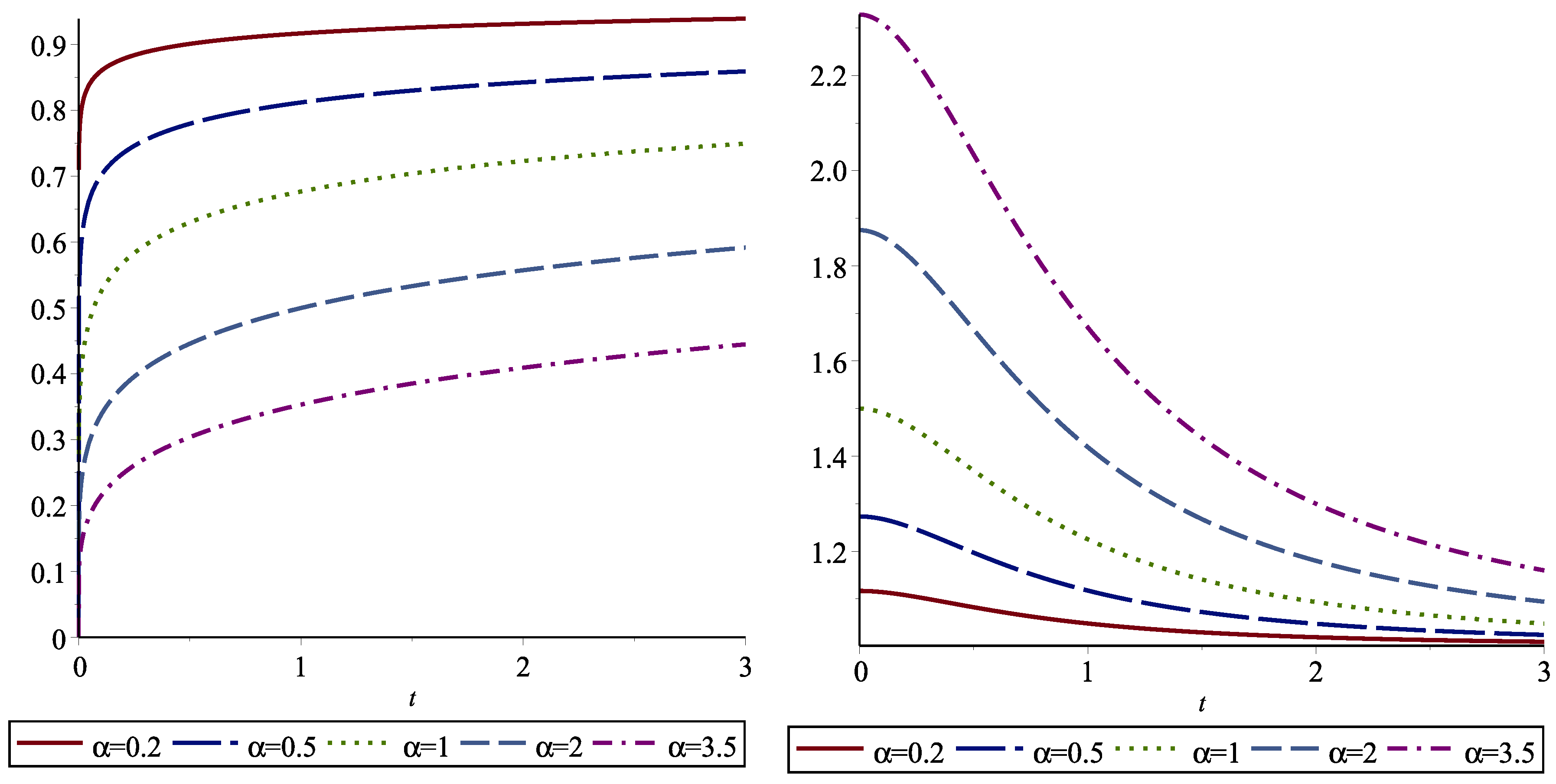
In
Table 4, we give the dynamically normalized FGCREs for some distributions. For example, we present the dynamically normalized FGCRE of the Weibull distribution in
Figure 3. We note that
X is IMRL when
and
X is DMRL when
Eventually, the inequalities given in (
25) can be developed as
The inequalities given above are very useful when the dynamic FGCRE has a complicated form.


