Abstract
In this paper, we present stochastic synchronous cellular automaton defined on a square lattice. The automaton rules are based on the SEIR (susceptible → exposed → infected → recovered) model with probabilistic parameters gathered from real-world data on human mortality and the characteristics of the SARS-CoV-2 disease. With computer simulations, we show the influence of the radius of the neighborhood on the number of infected and deceased agents in the artificial population. The increase in the radius of the neighborhood favors the spread of the pandemic. However, for a large range of interactions of exposed agents (who neither have symptoms of the disease nor have been diagnosed by appropriate tests), even isolation of infected agents cannot prevent successful disease propagation. This supports aggressive testing against disease as one of the useful strategies to prevent large peaks of infection in the spread of SARS-CoV-2-like diseases.
1. Introduction
Currently, the death rate of SARS-CoV-2 [1] in the whole world reached around 1.2% of the infected population and more than cases have been confirmed [2,3], (tab ‘Closed Cases’). Thus, one should not be surprised of the publication rash in this subject giving (i) theoretical bases of SARS-CoV-2 spreading, (ii) practical tips on preventing plagues or even (iii) clinical case studies making it easier to recognize and to treat cases of the disease. The Web of Science database reveals over 80,000 and over 110,000 papers related to this topic registered in 2020 and in January–November 2021, respectively, in contrast to only 19 papers in 2019. Among them, only several [4,5,6,7,8,9,10,11,12,13,14,15,16,17,18,19,20] are based on the cellular automata technique [21,22,23,24].
The likely reason for this moderate interest in using this technique to simulate the spread of the COVID-19 pandemic is the large degree of simplification of ‘rules of the game’ in cellular automata. To fill this gap, in this work, we propose a cellular automaton based on a compartmental model, the parameters of which were adjusted to the realistic probabilities of the transitions between the states of the automaton. Let us note that modeling the spread of the pandemic is also possible with other models (see [25,26,27,28] for mini-reviews) including, for instance, those based on the percolation theory [29].
The history of the application of compartmental models to the mathematical modeling of infectious diseases dates to the first half of the 20th century and works of Ross [30], Ross and Hudson [31,32], Kermack and McKendrick [33,34] and Kendall [35]; see, for instance, Ref. [36] for an excellent review. In the compartmental model, the population is divided into several (usually labeled) compartments so that the agent only remains in one of them and the sequences of transitions between compartments (label changes) are defined. For instance, in the classical SIR model, agents change their states subsequently from susceptible () via infected () to recovered () [33,34,37]. Infected agents can transmit the disease to their susceptible neighbors () with a given probability . The infected agent may recover () with probability . After recovering, the agents are immune and they can no longer be infected with the disease. These rules may be described by a set of differential equations:
where is the mean number of agents’ contacts in the neighborhood and , , represent the fraction of susceptible, infected, and recovered agents, respectively. Typically, the initial condition for Equation (1) is:
where is the initial fraction of infected agents (fraction of ‘Patients Zero’).
The transition rates between states (i.e., probabilities and ) may be chosen arbitrarily or they may correspond to the reciprocal of agents’ residence times in selected states. In the latter case, residence time may be estimated by clinical observations [38,39]. The probability describes the speed of disease propagation (infecting rate) while the value of is responsible for the frequency of getting better (recovering rate). In this approximation, the dynamics of the infectious class depends on the reproduction ratio:
The case of separates the phase when the disease dies out and the phase when the disease spreads among the members of the population.
Equation (1) describe a mean-field evolution, which simulates a situation in which all agents interact directly with each other. In low-dimensional spatial networks, the mean-field dynamics (1) is modified by diffusive mechanisms [40]. In a realistic situation, the diffusive mode of pandemic spreading is mixed with the mean-field dynamics, corresponding to nonlocal transmissions resulting from the mobility of agents [41].
We use the SEIR model [42,43], upon extending the SIR model, where an additional compartment (labeled ) is available and it corresponds to agents in the exposed state. The exposed agents are infected but unaware of it—they neither have symptoms of the disease nor have been diagnosed by appropriate tests. This additional state requires splitting the transition rate into and corresponding to transition rates (probabilities) after contact with the exposed agent in state and after contact with the infected agent in state , respectively. We would like to emphasize that both exposed (in state ) and infected (in state ) agents may transmit disease.
According to Equation (1), after recovering, the convalescent in state lives forever, which seems contradictory to the observations of the real world. Although the Bible Book of Genesis (5:5–27; 9:29) mentions seven men who lived over 900 years, in modern society—thanks to public health systems (and sometimes in spite of them)—contemporary living lengths beyond one hundred years are rather rare. Mortality tables [44] show some correlations between probability of death and age [45]. This observation was first published by Gompertz in 1825 [46]. According to Gompertz’s law, mortality f increases exponentially with the age a of the individual as:
where b and c are constants. Moreover, as we mentioned in the first sentence of the Introduction, people can also die earlier than Gompertz’s law implies. For example, an epidemic of fatal diseases increases the mortality rate. To take care of these factors in modeling disease propagation, we consider removing agents from the population. This happens with agents’ age-dependent probabilities and for healthy and ill people, respectively. The removed individual is immediately replaced with a newly born baby.
In this paper, we propose a cellular automaton based simultaneously on SEIR model of disease propagation and Gompertz’s law of mortality. In Section 2, the cellular automaton, its rules and the available site neighborhoods are presented. Section 3 is devoted to the presentation of the results of simulations based on the proposed cellular automaton. Discussion of the obtained results (Section 4) and conclusions (Section 5) end the paper. We note [47,48], where age-structured populations were also studied with SEIR-based and multicompartments models, respectively.
2. Model
We use the cellular automata technique [21,22,23,24] to model disease propagation. The cellular automata technique is based on several assumptions, including:
- Discrete (geometrical) space (i.e., regular lattice) and time;
- Discrete and finite set of available states of the single lattice’s site;
- Local rule of synchronous site states update.
The rule defines the state of the site i at time based on this site’s state at time t and the state of the sites in the i-th site’s neighborhood
We adopt the SEIR model for the simulation of disease spreading by probabilistic synchronous cellular automata on a square lattice with various neighborhoods . Every agent may be in one of four available states: susceptible (), exposed (), infected () or recovered (). The agents in and are characterized by different values of the probability of infection ( and ) and different ranges of interactions (radii of neighborhoods and ). The considered neighborhoods (and their radii) are presented in Figure 1.
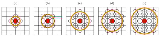
Figure 1.
Sites in various neighborhoods on a square lattice. (a) Von Neumann’s neighborhood (, ); (b) Moore’s neighborhood (, ); (c) neighborhood with sites up to the third coordination zone (, ); (d) neighborhood with sites up to the fourth coordination zone (, ); (e) neighborhood with sites up to the fifth coordination zone (, ).
Initially (at ), every agent is in the state, their age a is set randomly from a normal distribution with the mean value days and dispersion days. ‘Patient Zero’ in the state is placed randomly at a single site of a square lattice with nodes.
Every time step (which corresponds literally to a single day in the real-world) the lattice is scanned in typewriter order to check the possible agent state evolution:
- The susceptible agent may be infected () by each agent in state or present in his/her neighborhood with radius or , respectively. We set as we assume that infected (and aware of the disease) agents are more responsible than exposed (unaware of the disease) ones. The latter inequality comes from our assumption that the exposed agent is not careful enough in undertaking contacts with his/her neighbours while the infected agent is serious-minded and realizing the hazard of possible disease propagation and thus he/she avoids these contacts at least on the level assigned to exposed agents. The number and position of available neighbours who may infect the considered susceptible agent depend on the value of radius and/or as presented in Figure 1. The infection of the susceptible agents occurs with probability (after contacting with agent in state ) or (after contacting with agent in state ), respectively.
- The incubation (i.e., the appearance of disease symptoms) takes days—every agent in state is converted to infected state () with probability . The exposed agent may die with age-dependent probability . In such a case, he/she is replaced () with newly born agent ().
- The disease lasts for days. The ill agent (in state ) may either die (and be replaced by a newly born child ) with age specific probability or he/she can recover (and gain resistance to disease ) with probability .
- A healthy agent ( or ) may die with a chance given by age dependent probability . In such a case, it is replaced with a newly born susceptible baby (in state and in age of ).
The agents’ state modifications are applied synchronously to all sites. A single time step (from t to ) of the system evolution described above is presented in Algorithm 1. The -long vector variables tmp_pop[] and pop[] represent the current population (at time t) and the population in the next time step (), respectively. The presence of two such variables in a model implementation is caused by the synchronicity of cellular automaton. The i-th element of these vectors keeps information on the state (either or ) of the i-th agent in the population. The age a (measured in days) for the i-th agent is kept in the -long vector age[] and its i-th element is either incremented (line 4 of Algorithm 1) or reset (lines 28 and 35 of Algorithm 1) in the case of removal. The random() function returns a real pseudo-random number uniformly distributed in . The function measures the Euclidean distance between agents i and j. The age-dependent daily death probability functions and —based on real-world data—are defined in the next paragraph in Equations (5) and (6). The numbers , , and of agents in various states must be initialized at based on initial conditions. The cumulative number of deceased agents—earlier either in the exposed () or in the infected () state—is incremented in line 39 of Algorithm 1. The numbers , , , and are normalized to the total number of agents in the system before their return.
Based on American data on annual death probability [44] and assuming 365 days a year, we predict the daily death probability as:
where a is the agent’s age expressed in days. The data follow Gompertz’s exponential law of mortality [46,49].
Using the same trick, we estimate the probability of daily death for infected people of age a (expressed in days) as:
These probabilities are calculated as the chance of death during SARS-CoV-2 infection (based on Polish statistics [50]) divided by . We assume that infection lasts days and that an incubation process takes days [39]. Exponential fits (Equations (5) and (6)) to real-world data are presented in Figure 2.
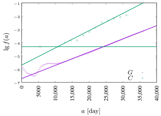
Figure 2.
Daily death probability for patients infected by the coronavirus (SARS-CoV-2, ×, , 50]) and natural death probability (+, , 44]).
| Algorithm 1: Single time step in automaton |
 |
3. Results
In Figure 3 snapshots from a single-run simulation are presented. They give a quantitative picture of the influence of the interaction range (neighborhood radius) on the spread of the disease. The snapshots in Figure 3a–e show the situation for fixed parameters and at the time step, which corresponds to five months after introducing (at random site) ‘Patient Zero’. The last subfigure (Figure 3f) presents a situation after a very long time of simulations ( 20,000) where the recovered agents die due to their age (according to Equation (5)) and are subsequently replaced by newly born children. For the interaction limited to the first coordination zone (Figure 1a) the disease propagation stays limited to the nearest neighbors of ‘Patient Zero’. On the other hand, for the neighborhood with sites up to the fifth coordination zone (Figure 1e) for the same infection rates ( and ) the disease affects all agents in the population (see Figure 3e). The direct evolution of the system based on [51] can be simulated and observed with the JavaScript application available at [52].
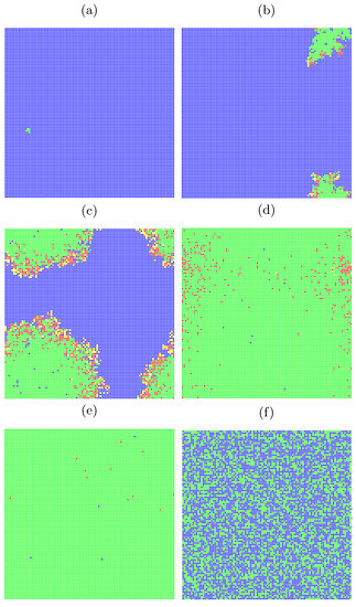
Figure 3.
Snapshots from direct simulation [52] for , , . The assumed ranges of interactions are (a) , (b) , (c) , (d,f) , and (e) . The simulation took time steps except for Figure 3f, where the situation after 20,000 time steps is presented.
In Figure 4 the fraction of infected agents (in state ) is presented. The figure shows the results of ten different simulations for values of the neighborhood radius , , . In addition, the results of averaging over simulations are presented. In two out of ten cases, the epidemic died out right after the start, while in the remaining eight cases it lasted from about eight hundred to over a thousand time steps (days). The figure also shows that the averaging of the results allows for a significant smoothing of the curves, which fluctuate strongly for individual simulations. Based on this test (for (not shown) roughly doubly large statistics, , which do not reveal significant deviations), we decided to average our results (presented in Figure 5, Figure 6 and Figure 7) over ten independent simulations.
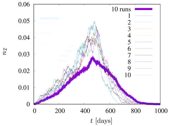
Figure 4.
Ten different simulations for values of the neighborhood radius = 1.5. , .
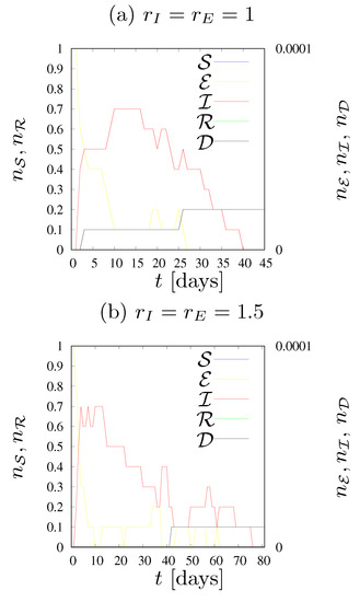
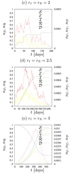
Figure 5.
Dynamics of states fractions for various values of the neighborhood radius . , .
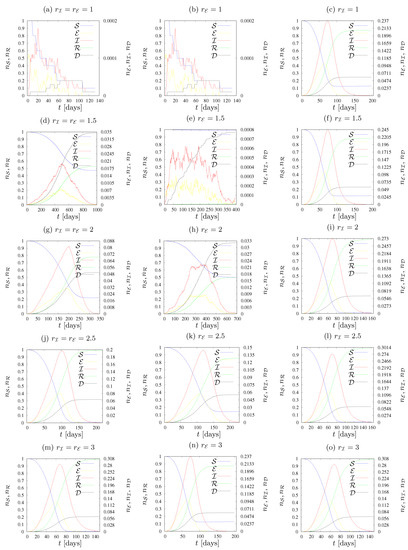
Figure 6.
Dynamics of states fractions for various values of the neighborhood radius (left) , (middle) , (right) . , , .
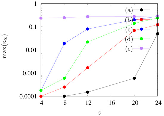
Figure 7.
Maximal fraction of agents in state as dependent on the number of agents’ neighbours z in the neighborhood. (a) , , (b) , , (c) , , , (d) , , , , (e) , , , .
The diagrams in Figure 5 and Figure 6 show the evolution of the epidemic. Namely, they show the number of agents in each state on each day of the epidemic, as well as the cumulative fraction of deaths (). The fraction of susceptible agents and the fraction of recovered agents are shown on the left vertical axis, while the fractions of exposed agents and of infected agents and the cumulative fraction of deaths caused by infection are shown on the right vertical axis.
3.1.
The case of (corresponding to total lockdown) leads to immediate disease dieout as only ‘Patients Zero’ at are infected and recover after about ∼ time steps (days) depending on the agent’s age a.
3.2.
In Figure 5 the dynamics of states fractions n for various values of the neighborhood radius are presented. We assume infection rates . The assumed transition rates and are very low. As a result, the disease has a very limited chance of spreading in society.
Figure 5a illustrates the situation where an infected person (independently either in the or states) can only infect the four closest neighbors. The epidemic lasted a maximum of forty days, the number of agents who were ill at the same time was less than one (on average, in ten simulations), there were only two deaths out of ten simulations, and the population was not affected by the disease.
The case presented in Figure 5b illustrates the situation in which each person can infect up to eight neighbors. This does not cause significant changes during the epidemic compared with Figure 5a; the average number of simultaneously ill agents remained below one, this time only one person in ten simulations died due to SARS-CoV-2 infection, and the duration of the epidemic was approximately 75 days—twice longer than presented in Figure 5a. We would like to emphasize that the term ‘duration of the epidemic’ determines the time of the longest duration of the epidemic among the ten simulations carried out.
Figure 5c shows the situation where there were twelve agents in the neighborhood of each cell. The transition rates ( and ) turned out to be so low, that—despite extending the neighborhood—the epidemic vanished quickly. This time the fractions of exposed and infected agents were slightly higher, the maximum number of sick agents in one day was more than one, the longest simulation lasted 80 days, and four agents died within ten iterations.
Increasing the radius of the neighborhood to 2.5 (see Figure 5d) increased the number of exposed and infected agents more than twice compared to Figure 5c. On the day of the peak of the epidemic, five agents were sick and seven died during the epidemic (on average). The epidemic lasted about 600 days, but only about 1–2% of the population became infected throughout the epidemic.
Only an increase in the number of agents in the neighborhood to 24 (as presented in Figure 5e) caused a smooth and rapid development of the epidemic. In this case, it lasted about 550 days, the largest number of sick agents in one day was approximately 500, and the same number of agents also died throughout the epidemic. During the epidemic, around 75% of the population became infected.
In the left column of Figure 6 the dynamics of states fractions n for various values of the radius of the neighborhood are presented. We assume , . As we still keep , setting simulates the fact that exposed agents (who are not aware of their infection) are more dangerous to those around them than those who know that they are sick, and therefore avoid contact if they show severe symptoms of the disease.
In Figure 6a the results for the smallest possible neighborhood radius is presented. As in the previous cases with , the epidemic stopped quite quickly. The largest number of agents who were ill () at the same time was two, the longest simulation time was 120 days, the average number of deaths was well below one, and totally only a few agents were infected (the curve representing agents in the state of is almost not visible).
Figure 6d shows that contact with eight agents in the neighborhood (for assumed values of infection rates and ) is enough for the pandemic to affect society to a very large extent and last for a long time. The longest simulation took about 1000 days. During the epidemic, almost half of the population was infected, approximately 350 agents died, and at epidemic peak there were just over 180 sick agents in a single day.
Increasing the range of interaction to the next coordination zone (see Figure 6g) caused a significant reduction in the duration of the epidemic, as well as causing greater havoc among agents. In approximately 350 days, roughly 75% of the population was infected, approximately 500 died, and up to 800 were sick on the day when this number was highest.
Increasing the radius to 2.5, as shown in Figure 6j, further shortened the epidemic time, this time to just two hundred days. Almost all agents were infected, slightly more than 600 agents died, and the maximum number of patients on one day was 2000, which is as much as 20% of the population. Every fifth person was infected by the disease on that day, and if one adds about 800 agents who were in the exposed state , we get a situation where more than one quarter of the population is under the influence of this disease at the same time.
Further increasing the range of interactions (to the fifth coordination zone and 24 neighbors in it, shown in Figure 6m) gave very similar results to the previous one, except that the virus spread even faster, in less than 150 days. The number of deaths was similar (a little below 600), almost all agents had contact with the disease at some stage of the pandemic, and the maximum number of sick agents in one day was 2800. If one adds over 1100 agents in the state on the same day, the effect is that the disease affected nearly 40% of agents on the same day.
3.3.
In the middle column of Figure 6 the dynamics of the state fractions , , , for various values of the neighborhood radius are presented. We assume and . For this set of plots, has been predefined as 1 and only changes. Translating this into a description of the real world, sick agents who have disease symptoms are aware of their illness (infected) and limit their contact with the environment to a minimum, while oblivious agents (exposed) do not realize that they can transmit the disease. In each of the tested parameter sets, agents in the state can infect only four of their closest neighbors.
The plot in Figure 6e shows the situation where agents in the state can infect up to eight agents in their neighborhood. We see irregularities in the shapes of the curves showing the fraction of agents in the states and , and the duration of the epidemic is relatively long, over 400 days. However, the values shown in the graphs show that the pandemic was not dangerous for the entire population. Death from the disease was recorded on average in less than eight agents, the maximum number of sick agents in one day was just over six, and the total number of infected agents in the entire epidemic was so low that the deviation of the curve representing the number of agents in the state from the top of the graph is almost imperceptible.
In Figure 6h, the plots for further extension (to the third coordination zone, with neighbors) of the radius of the neighborhood of exposed agents (in the state ) are presented. The curves are much smoother than those presented in Figure 6e; however, we can still see some irregularities in the curves describing agents in the and states. The duration of the longest simulation was approximately 700 days, the number of deaths was less than 330, and at the peak of the pandemic, approximately 220 agents were simultaneously ill. The curves presenting the fraction of agents in the states of and almost perfectly line up on the right side of the chart, meaning that half of the population contracted the disease while the other half remained healthy throughout the epidemic.
The case where agents in the state can infect agents within a radius of 2.5 is shown in Figure 6k. The epidemic was definitely more dynamic than in the previously studied case (Figure 6h), lasting only a little over two hundred days, and the maximum number of sick agents in one day reached almost 1500 agents. The sum of those who died from the coronavirus was less than 600, and during the pandemic, approximately 85% of the population became recovered (and earlier exposed and/or infected).
Finally, for the radius increased to three (see Figure 6n) we did not observe too many changes compared to the previous case (Figure 6k). The epidemic was even shorter, it lasted a little more than 150 days, the number of deaths was very similar (it could be estimated at 600), slightly more than 85% of agents in the population were infected, and at the hardest moment of the pandemic there were at the same time about 2370 sick agents (in the state). The results are therefore almost identical to those of , except that disease propagation is faster.
The right column of Figure 6 shows cases with predetermined and various . We keep and
All graphs are very similar to each other, as a large range of infections of agents in the state makes the influence of on epidemic evolution only marginal. This can be easily observed by comparing the scales presented in all subfigures. The assumed range of infection is large enough (at least for assumed values of transmission rates and ) to prevent any observable influence of on epidemic trajectories.
4. Discussion
Let us start the discussion with comparing the leftmost (Figure 6a,d,g,j,m) and the middle (Figure 6b,e,h,k,n) columns of Figure 6. The comparison reveals that quarantining or limiting the connectivity of agents in the state (both infected and informed) may bring good or even very good results in preventing disease propagation, depending on the arrangement of the other parameters. For , this completely brought the epidemic to a halt, which would otherwise affect more than half the population. With , it makes it possible to reduce the share of infected agents in the population from 75% to 50%. The effects on and are similar—instead of the total population, less than 90% of population became infected. When the pandemic duration was significantly shortened, it is because the virus was unable to survive, and the disease was extinct. In other cases, the duration of the epidemic increased; the restrictions introduced for agents in the state did not completely extinguish the disease, but allowed to slow it down and mitigate its effects.
For low values of the probability of infection (), that is, in a situation where the transmission of the virus is not too high, even a slight limitation of the contact among agents allows for a complete inhibition of the disease and protection of the society against its negative effects (see Figure 5). We note that manipulating the and/or parameters may reflect changes in disease transition rates with their low values corresponding to wild variant of the SARS-CoV-2 virus while higher values correspond to the fiercer (including delta and specially omicron) variants of the SARS-CoV-2 virus. For instance, for a fixed radius of interaction () for low values of nearly 75% of the population reached the state (Figure 5e) while increasing infection rates to and caused the entire population to fall ill (Figure 6m). The summed values of the fractions of exposed and infected agents at the peaks of disease are 6.6% (for , Figure 5e) and 39% (for and , Figure 6m) of the population.
The results presented in Figure 5 and Figure 6 are summarized in Figure 7, where the maximum fraction of agents in state vs. the neighbours number z for various sets of parameters is presented. We observe a gradual increase in the maximum number of infected agents (up to 30%) as the number of agents in the neighborhood increases. An exception to this rule is observed only when , when the maximum level of infections is constant and it does not change with the increase of the range of the interaction of agents in state .
5. Conclusions
In this article we present a stochastic synchronous cellular automaton defined on a square lattice. The automaton rules are based on the SEIR model with probabilistic parameters collected from real human mortality data and SARS-CoV-2 disease characteristics. Automaton rules are presented in Algorithm 1. With computer simulations, we show the influence of the radius of the neighborhood on the number of infected and deceased agents in the artificial population.
The study presented in this paper is based on static automaton. Thus, our approach is equivalent to disease propagation described in terms of conduction-like processes (i.e., the position of each cell is fixed and can infect a neighbor, at distance or ). The latter is a natural way to model with the cellular automata technique. However, we note that also convection-like processes (i.e., the population can flow within the system) may play a crucial role at both large [53] and local scales [19,54].
Further enrichment of the model can lead to the introduction of additional components, including the compartment that describes the vaccinated agents. This model improvement allows us to study scenarios with limited and unlimited vaccine supply [20] or the existence and stability of steady states [55,56]. Vaccinations seem to be particularly effective when the vaccination campaign starts early and with a large number of vaccinated individuals [20]. Moreover, the realistic models should take into account people’s attitudes to vaccination programs [57,58].
In conclusion, increasing the radius of the neighborhood (and the number of agents interacting locally) favors the spread of the epidemic. However, for a wide range of interactions of exposed agents, even isolation of infected agents cannot prevent successful disease propagation. This supports aggressive testing against disease as one of the useful strategies to prevent large peaks of infection in the spread of SARS-CoV-2-like disease. The latter can have devastating consequences for the health care system, in particular for the availability of hospital beds for SARS-CoV-2 and other diseases.
Author Contributions
Conceptualization, K.M.; Investigation, S.B.; Methodology, K.M.; Software, S.B.; Visualization, S.B.; Writing-original draft, K.M.; Writing-review & editing, S.B. and K.M. All authors have read and agreed to the published version of the manuscript.
Funding
This research received no external funding.
Data Availability Statement
The theoretical data generated by cellular automata simulations is available from the authors upon a reasonable request. The real-world data is based on [44,50].
Acknowledgments
The authors are grateful to Zdzisław Burda for critical reading of the manuscript and fruitful discussion.
Conflicts of Interest
The authors declare no conflict of interest.
References
- Zhu, N.; Zhang, D.; Wang, W.; Li, X.; Yang, B.; Song, J.; Zhao, X.; Huang, B.; Shi, W.; Lu, R.; et al. A novel coronavirus from patients with pneumonia in China, 2019. N. Engl. J. Med. 2020, 382, 727–733. [Google Scholar] [CrossRef] [PubMed]
- WHO COVID-19 Dashboard; World Health Organization: Geneva, Switzerland, 2020; Available online: https://covid19.who.int/ (accessed on 1 June 2021).
- Worldometers: COVID-19 Coronavirus Pandemic. 2021. Available online: https://www.worldometers.info/coronavirus/ (accessed on 1 December 2021).
- Zhang, Y.; Gong, C.; Li, D.; Wang, Z.-W.; Pu, S.D.; Robertson, A.W.; Yu, H.; Parrington, J. A prognostic dynamic model applicable to infectious diseases providing easily visualized guides: A case study of COVID-19 in the UK. Sci. Rep. 2021, 11, 8412. [Google Scholar] [CrossRef] [PubMed]
- Lima, L.L.; Atman, A.P.F. Impact of mobility restriction in COVID-19 superspreading events using agent-based model. PLoS ONE 2021, 16, e0248708. [Google Scholar] [CrossRef] [PubMed]
- Medrek, M.; Pastuszak, Z. Numerical simulation of the novel coronavirus spreading? Expert Syst. Appl. 2021, 166, 114109. [Google Scholar] [CrossRef]
- Schimit, P.H.T. A model based on cellular automata to estimate the social isolation impact on COVID-19 spreading in Brazil. Comput. Methods Programs Biomed. 2021, 200, 105832. [Google Scholar] [CrossRef]
- Dai, J.; Zhai, C.; Ai, J.; Ma, J.; Wang, J.; Sun, W. Modeling the spread of epidemics based on cellular automata. Processes 2021, 9, 55. [Google Scholar] [CrossRef]
- Zupanc, G.K.H.; Lehotzky, D.; Tripp, I.P. The neurosphere simulator: An educational online tool for modeling neural stem cell behavior and tissue growth. Dev. Biol. 2021, 469, 80–85. [Google Scholar] [CrossRef]
- Gwizdalla, T. Viral disease spreading in grouped population. Comput. Methods Progrems Biomed. 2020, 197, 105715. [Google Scholar] [CrossRef]
- Monteiro, L.H.A.; Fanti, V.C.; Tessaro, A.S. On the spread of SARS-CoV-2 under quarantine: A study based on probabilistic cellular automaton. Ecol. Complex. 2020, 44, 100879. [Google Scholar] [CrossRef]
- Ghosh, S.; Bhattacharya, S. A data-driven understanding of COVID-19 dynamics using sequential genetic algorithm based probabilistic cellular automata. Appl. Soft Comput. 2020, 96, 106692. [Google Scholar] [CrossRef]
- Zhou, Y.; Li, J.; Chen, Z.; Luo, Q.; Wu, X.; Ye, L.; Ni, H.; Fei, C. The global COVID-19 pandemic at a crossroads: Relevant countermeasures and ways ahead. J. Thorac. Dis. 2020, 12, 5739–5755. [Google Scholar] [CrossRef] [PubMed]
- Mondal, S.; Mukherjee, S.; Bagchi, B. Mathematical modeling and cellular automata simulation of infectious disease dynamics: Applications to the understanding of herd immunity. J. Chem. Phys. 2020, 153, 114119. [Google Scholar] [CrossRef] [PubMed]
- Tang, L.; Zhou, Y.; Wang, L.; Purkayastha, S.; Zhang, L.; He, J.; Wang, F.; Song, P.X.-K. A review of multi-compartment infectious disease models. Int. Stat. Rev. 2020, 88, 462–513. [Google Scholar] [CrossRef] [PubMed]
- Yuan, M. Geographical information science for the United Nations’ 2030 agenda for sustainable development. Int. J. Geogr. Inf. Sci. 2021, 35, 1–8. [Google Scholar] [CrossRef]
- Dascalu, M.; Malita, M.; Barbilian, A.; Franti, E.; Stefan, G.M. Enhanced cellular automata with autonomous agents for COVID-19 pandemic modeling. Rom. J. Inf. Sci. Technol. 2020, 23, S15–S27. [Google Scholar]
- Orzechowska, J.; Fordon, D.; Gwizdałła, T. Size effect in cellular automata based disease spreading model. Lect. Notes Comput. Sci. 2018, 11115, 146–153. [Google Scholar]
- Nava, A.; Papa, A.; Rossi, M.; Giuliano, D. Analytical and cellular automaton approach to a generalized SEIR model for infection spread in an open crowded space. Phys. Rev. Res. 2020, 2, 043379. [Google Scholar] [CrossRef]
- Gabrick, E.C.; Protachevicz, P.R.; Batista, A.M.; Iarosz, K.C.; de Souza, S.L.; Almeida, A.C.; Szezech, J.D.; Mugnaine, M.; Caldas, I.L. Effect of two vaccine doses in the SEIR epidemic model using a stochastic cellular automaton. Phys. A Stat. Mech. Its Appl. 2022, 597, 127258. [Google Scholar] [CrossRef]
- Ilachinski, A. Cellular Automata: A Discrete Universe; World Scientific: Singapore, 2001. [Google Scholar]
- Wolfram, S. A New Kind of Science; Wolfram Media; Available online: https://www.wolfram-media.com/ (accessed on 1 December 2021).
- Chopard, B.; Droz, M. Cellular Automata Modeling of Physical Systems; Cambridge University Press: Cambridge, UK, 2005. [Google Scholar]
- Chopard, B. Computational Complexity: Theory, Techniques, and Applications; Meyers, R.A., Ed.; Springer: New York, NY, USA, 2012; pp. 407–433. [Google Scholar]
- de Oliveira, P.M.C. Epidemics a la Stauffer. Phys. A Stat. Mech. Its Appl. 2021, 561, 125287. [Google Scholar] [CrossRef]
- Lux, T. The social dynamics of COVID-19. Phys. A Stat. Mech. Its Appl. 2021, 567, 125710. [Google Scholar] [CrossRef]
- Weisbuch, G. Urban exodus and the dynamics of COVID-19 pandemics. Phys. A Stat. Mech. Its Appl. 2021, 569, 125780. [Google Scholar] [CrossRef] [PubMed]
- Lorig, F.; Johansson, E.; Davidsson, P. Agent-based social simulation of the COVID-19 pandemic: A systematic review. J. Artif. Soc. Soc. Simul. 2021, 24, 5. [Google Scholar] [CrossRef]
- Ziff, R.M. Percolation and the pandemic. Phys. A Stat. Mech. Its Appl. 2021, 568, 125723. [Google Scholar] [CrossRef]
- Ross, R. An application of the theory of probabilities to the study of a priori pathometry—Part I. Proc. R. Soc. Lond. 1916, 92, 204–230. [Google Scholar]
- Ross, R.; Hudson, H.P. An application of the theory of probabilities to the study of a priori pathometry—Part II. Proc. R. Soc. Lond. 1917, 93, 212–225. [Google Scholar]
- Ross, R.; Hudson, H.P. An application of the theory of probabilities to the study of a priori pathometry—Part III. Proc. R. Soc. Lond. 1917, 93, 225–240. [Google Scholar]
- Kermack, W.O.; McKendrick, A.G. A contribution to the mathematical theory of epidemics. Proc. R. Soc. Lond. 1927, 115, 700–721. [Google Scholar]
- Kermack, W.O.; McKendrick, A.G. Contributions to the mathematical theory of epidemics—I. Bull. Math. Biol. 1991, 53, 33–55. [Google Scholar]
- Kendall, D.G. Berkeley Symposium on Mathematical Statistics and Probability; University of California Press: Berkeley, CA, USA, 1956; pp. 149–165. [Google Scholar]
- Hethcote, H.W. The mathematics of infectious diseases. SIAM Rev. 2000, 42, 599–653. [Google Scholar] [CrossRef]
- Newman, M.E.J. Spread of epidemic disease on networks. Phys. Rev. E 2002, 66, 016128. [Google Scholar] [CrossRef]
- Worldometers: COVID-19 Coronavirus Pandemic. 2021. Available online: https://www.worldometers.info/coronavirus/coronavirus-symptoms/ (accessed on 1 December 2021).
- Worldometers: COVID-19 Coronavirus Pandemic. 2021. Available online: https://www.worldometers.info/coronavirus/coronavirus-incubation-period/ (accessed on 1 December 2021).
- Barthélemy, M. Spatial networks. Phys. Rep. 2011, 499, 1–101. [Google Scholar] [CrossRef]
- Burda, Z. Modelling excess mortality in COVID-19-like epidemics. Entropy 2020, 22, 1236. [Google Scholar] [CrossRef] [PubMed]
- Dureau, J.; Kalogeropoulos, K.; Baguelin, M. Capturing the time-varying drivers of an epidemic using stochastic dynamical systems. Biostatistics 2013, 14, 541–555. [Google Scholar] [CrossRef]
- Faranda, D.; Alberti, T. Modeling the second wave of COVID-19 infections in France and Italy via a stochastic SEIR model. Chaos Interdiscip. J. Nonlinear Sci. 2020, 30, 111101. [Google Scholar] [CrossRef] [PubMed]
- Arias, E. United States life tables, 2003. Natl. Vital Stat. Rep. 2006, 54, 1–40. [Google Scholar] [PubMed]
- Richmond, P.; Roehner, B.M.; Irannezhad, A.; Hutzler, S. Mortality: A physics perspective. Phys. A Stat. Mech. Its Appl. 2021, 566, 125660. [Google Scholar] [CrossRef]
- Gompertz, B. On the nature of the function expressive of the law of human mortality, and on a new mode of 11 determining the value of life contingencies. Philos. Trans. R. Soc. Lond. 1825, 115, 513–583. [Google Scholar]
- Vandamme, L.K.J.; Rocha, P.R.F. Analysis and simulation of epidemic COVID-19 curves with the Verhulst model applied to statistical inhomogeneous age groups. Appl. Sci. 2021, 11, 4159. [Google Scholar] [CrossRef]
- Filho, T.M.R.; Moret, M.A.; Chow, C.C.; Phillips, J.C.; Cordeiro, A.J.A.; Scorza, F.A.; Almeida, A.-C.G.; Mendes, J.F.F. A data-driven model for COVID-19 pandemic—Evolution of the attack rate and prognosis for Brazil. Chaos Solitons Fractals 2021, 152, 111359. [Google Scholar] [CrossRef]
- Makowiec, D.; Stauffer, D.; Zielinski, M. Gompertz law in simple computer model of aging of biological population. Int. J. Mod. Phys. C 2001, 12, 1067–1073. [Google Scholar] [CrossRef]
- Distribution of Deaths Due to the Coronavirus (COVID-19) in Poland as of January 2021, by Age Group. Data Based on National Institute of Public Health PZH Report (in Polish). 2021. Available online: https://www.statista.com/statistics/1110890/poland-coronavirus-covid-19-fatalities-by-age/ (accessed on 1 March 2022). [CrossRef]
- Biernacki, S. Computer Simulation of the Impact of Quarantine and Limitation of Long-Range Communication on the Spread of an Epidemic of a Drop-Borne Virus. Master’s Thesis, AGH University of Science and Technology, Kraków, Poland, 2021. [Google Scholar]
- Biernacki, S. Javascript Application. Available online: http://www.zis.agh.edu.pl/app/MSc/Szymon_Biernacki/ (accessed on 1 December 2021).
- Belik, V.; Geisel, T.; Brockmann, D. Natural human mobility patterns and spatial spread of infectious diseases. Phys. Rev. X 2011, 1, 011001. [Google Scholar] [CrossRef]
- Mello, B.A. One-way pedestrian traffic is a means of reducing personal encounters in epidemics. Front. Phys. 2020, 8, 376. [Google Scholar] [CrossRef]
- Sun, D.; Li, Y.; Teng, Z.; Zhang, T.; Lu, J. Dynamical properties in an SVEIR epidemic model with age-dependent vaccination, latency, infection, and relapse. Math. Methods Appl. Sci. 2021, 44, 12810–12834. [Google Scholar] [CrossRef]
- Nabti, A.; Ghanbari, B. Global stability analysis of a fractional SVEIR epidemic model. Math. Methods Appl. Sci. 2021, 44, 8577–8597. [Google Scholar] [CrossRef]
- Bier, M.; Brak, B. A simple model to quantitatively account for periodic outbreaks of the measles in the Dutch Bible Belt. Eur. Phys. J. 2015, 88, 107. [Google Scholar] [CrossRef][Green Version]
- Lisowski, B.; Yuvan, S.; Bier, M. Outbreaks of the measles in the Dutch Bible Belt and in other places—New prospects for a 1000 year old virus. Biosystems 2019, 177, 16–23. [Google Scholar] [CrossRef]
Publisher’s Note: MDPI stays neutral with regard to jurisdictional claims in published maps and institutional affiliations. |
© 2022 by the authors. Licensee MDPI, Basel, Switzerland. This article is an open access article distributed under the terms and conditions of the Creative Commons Attribution (CC BY) license (https://creativecommons.org/licenses/by/4.0/).