Adaptive Hurst-Sensitive Active Queue Management

 , , , , and
Abstract
:1. Introduction
2. State of the Art
3. Hurst Estimation Methods
- —the process is negatively correlated, which means that the Long-Range Dependence does not occur;
- —the process is uncorrelated;
- —the process is positively correlated, which means that the LRD occurs.
4. Adaptive AQM
5. Selection of the AQM Parameters with the Use of Neural Networks
Adaptive Neuron AQM
6. Results
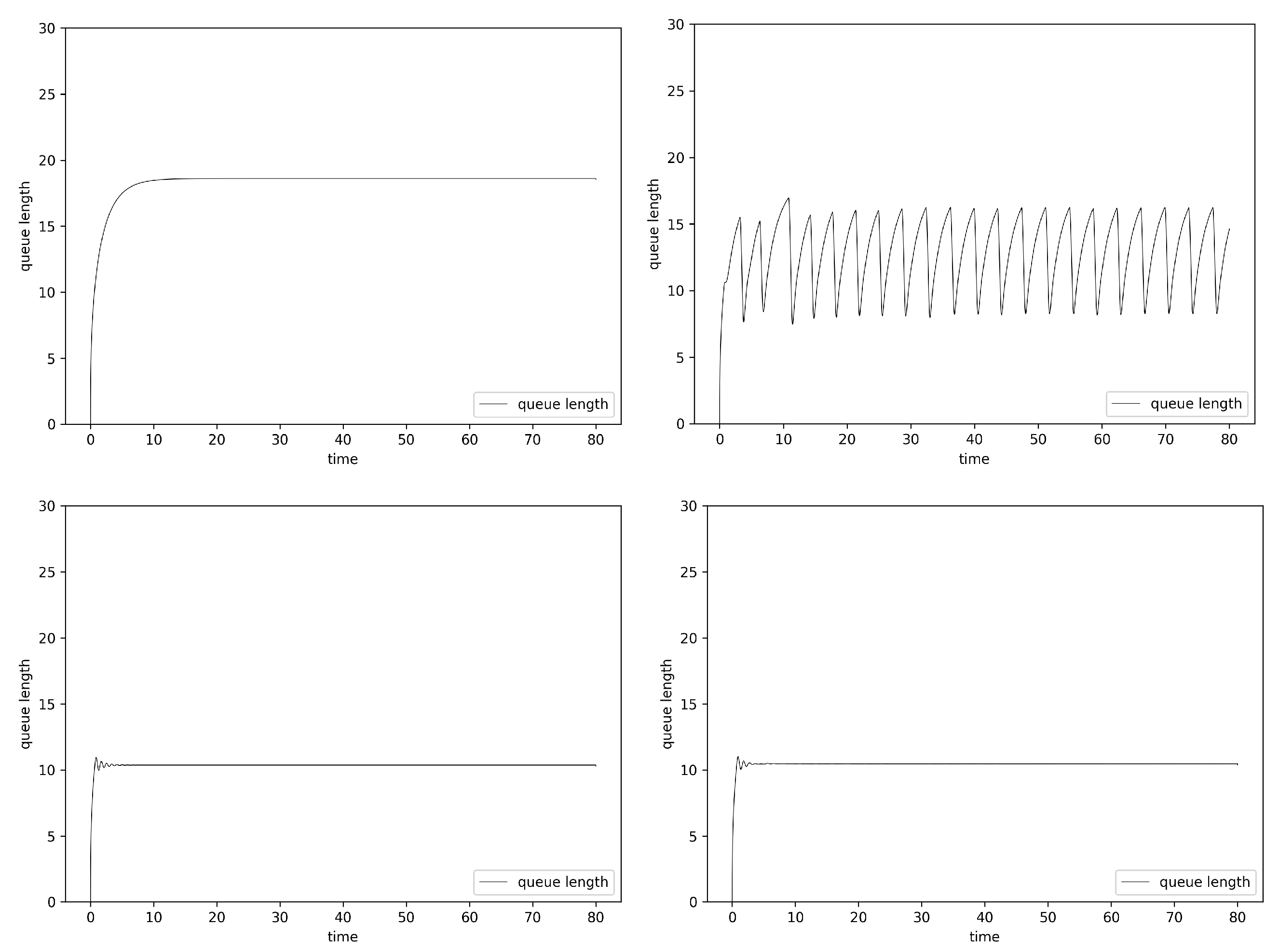
6.1. Fluid Flow Analysis
- is the expected TCP congestion window size (in packets) for the i-th flow. It defines a number of packets that may be sent without waiting for the acknowledgements of the reception of previous packets;
- is the round-trip time, , the sum denotes the total input flow to the congestion router;
- q is queue length (in packets);
- C is link capacity (packets/time unit), the constant output flow of the router;
- is propagation delay;
- N is the number of TCP sessions passing through the router;
- p is the packet drop probability.
- transmission capacity of AQM router: ;
- propagation delay for i-th flow: ;
- starting time for i-th flow (TCP and UDP);
- the number of packets sent by i-th flow (TCP and UDP).
- ;
- ;
- buffer size (measured in packets) ;
- ;
- eight parameter .
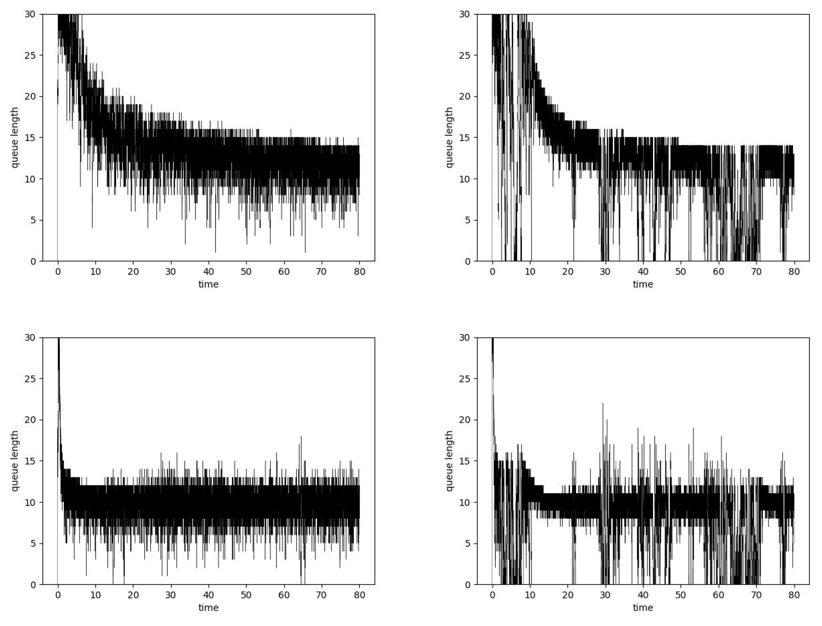
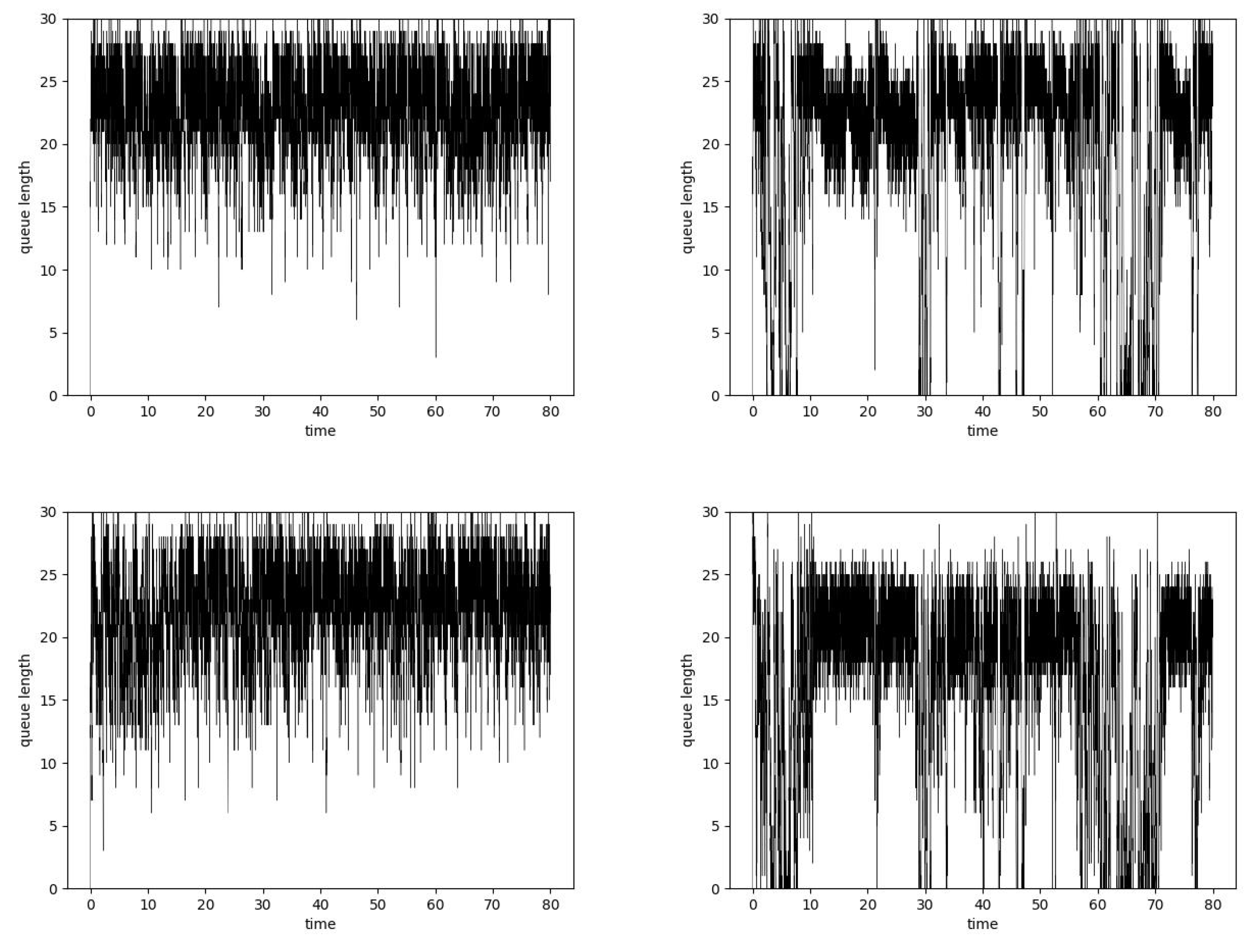
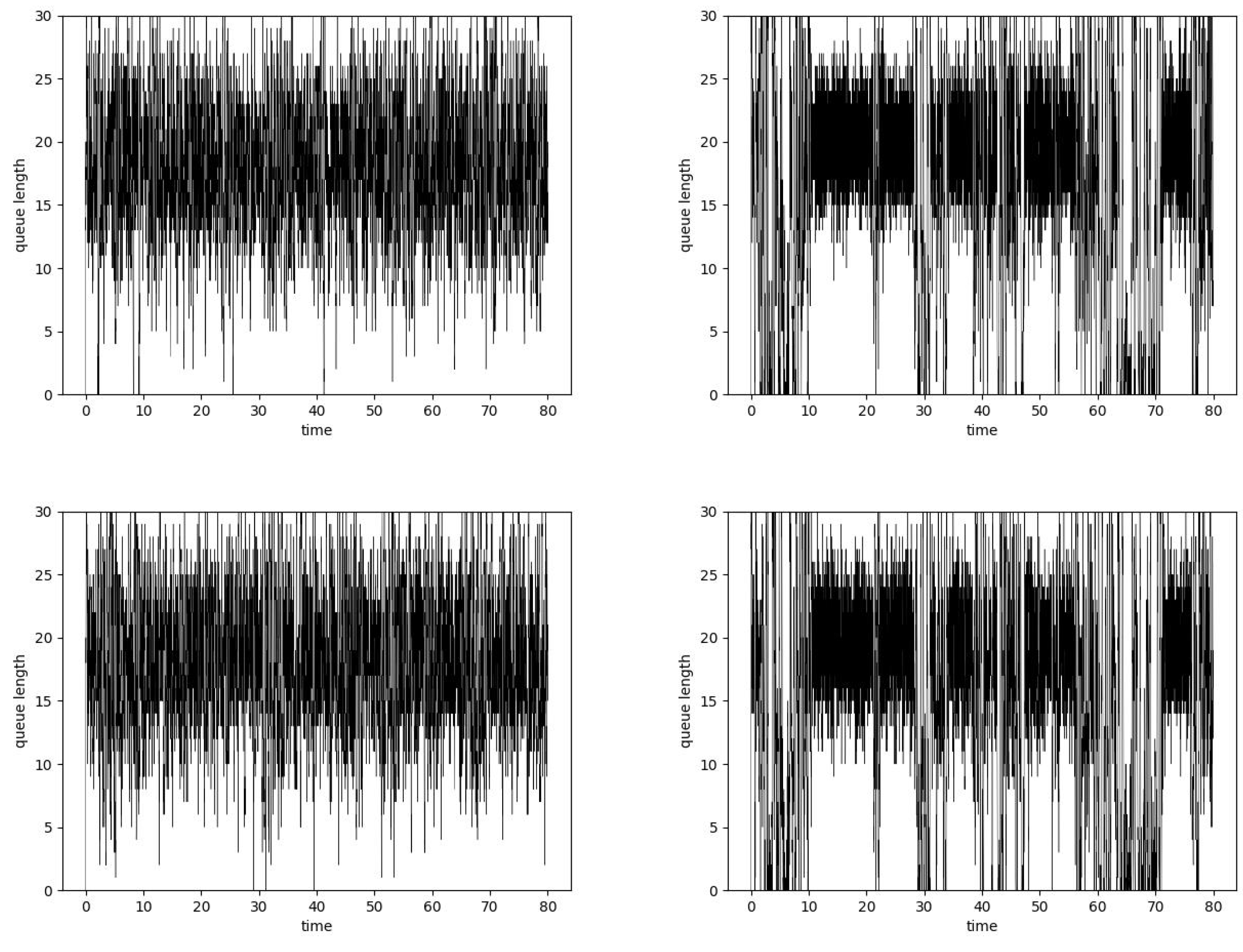
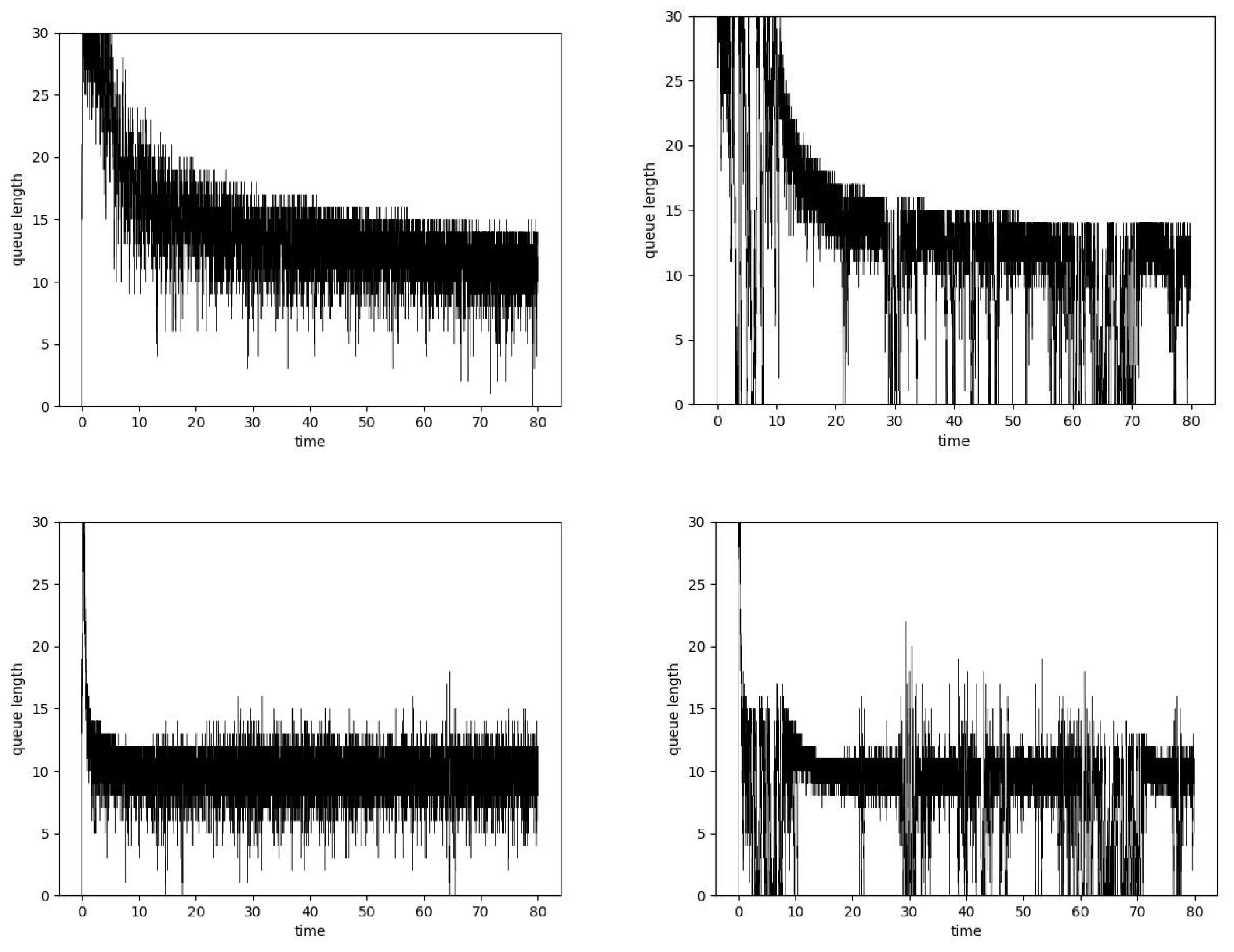
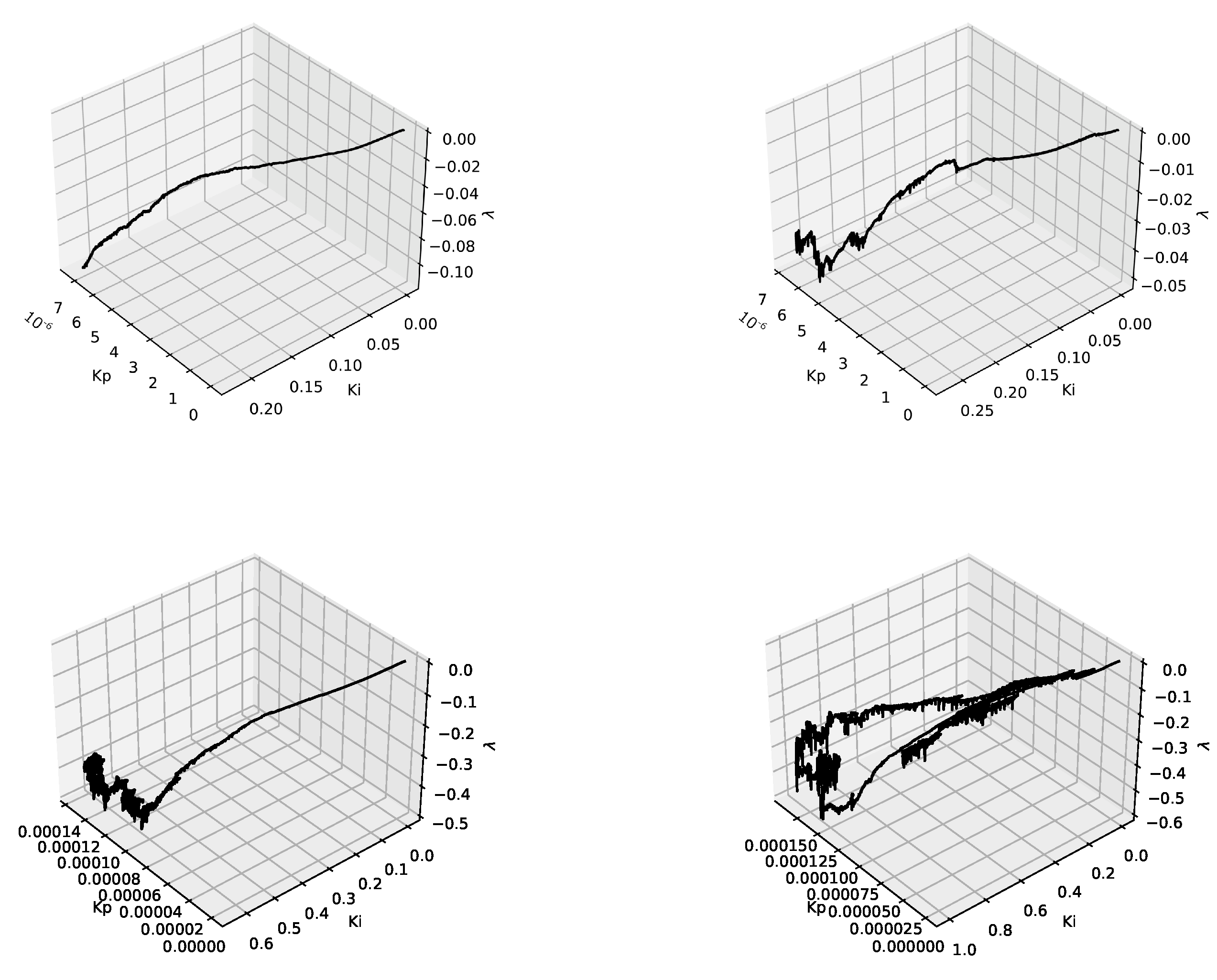
6.2. Simulation
7. Conclusions
Author Contributions
Funding
Institutional Review Board Statement
Informed Consent Statement
Data Availability Statement
Conflicts of Interest
References
- Larionov, A.; Vishnevsky, V.; Semenova, O.; Dudin, A. A multiphase queueing model for performance analysis of a multi-hop IEEE 802.11 wireless network with DCF channel access. In Proceedings of the International Conference on Information Technologies and Mathematical Modelling, Saratov, Russia, 26–30 June 2019; Springer: Berlin, Germany, 2019; pp. 162–176. [Google Scholar]
- Chisci, G.; ElSawy, H.; Conti, A.; Alouini, M.S.; Win, M.Z. Uncoordinated massive wireless networks: Spatiotemporal models and multiaccess strategies. IEEE/ACM Trans. Netw. 2019, 27, 918–931. [Google Scholar] [CrossRef]
- Swami, N.; Bairwa, A.; Choudhary, M. A Literature Survey of Network Simulation Tools. In IJCRT International Conference Proceeding ICCCT; Association for Computing Machinery: New York, NY, USA, 2017; Volume 5, pp. 206–208. [Google Scholar]
- Borboruah, G.; Nandi, G. A Study on Large Scale Network Simulators. Int. J. Comput. Sci. Inf. Technol. 2014, 5, 7318–7322. [Google Scholar]
- Dou, Y.; Liu, H.; Wei, L.; Chen, S. Design and simulation of self-organizing network routing algorithm based on Q-learning. In Proceedings of the 21st Asia-Pacific Network Operations and Management Symposium (APNOMS), Daegu, Korea, 22–25 September 2020; pp. 357–360. [Google Scholar] [CrossRef]
- Guo, X.; Guo, B.; Li, K.; Fan, C.; Yang, H.; Huang, S. A SDN-enabled Integrated Space-Ground Information Network Simulation Platform. In Proceedings of the 18th International Conference on Optical Communications and Networks (ICOCN), Huangshan, China, 5–8 August 2019; pp. 1–3. [Google Scholar] [CrossRef]
- Adamu, A.; Shorgin, V.; Melnikov, S.; Gaidamaka, Y. Flexible Random Early Detection Algorithm for Queue Management in Routers. In Proceedings of the International Conference on Distributed Computer and Communication Networks, Moscow, Russia, 14–18 September 2020; Springer: Berlin, Germany, 2020; pp. 196–208. [Google Scholar]
- Bisoy, S.K.; Pattnaik, P.K. A neuron-based active queue management scheme for internet congestion control. Int. J. Reason.-Based Intell. Syst. 2020, 12, 238–247. [Google Scholar]
- Floyd, S.; Jacobson, V. Random Early Detection gateways for congestion avoidance. IEEE/ACM Trans. Netw. 1993, 1, 397–413. [Google Scholar] [CrossRef]
- Tan, L.; Zhang, W.; Peng, G.; Chen, G. Stability of TCP/RED systems in AQM routers. IEEE Trans. Autom. Control 2006, 51, 1393–1398. [Google Scholar] [CrossRef]
- Unal, H.; Melchor-Aguilar, D.; Ustebay, D.; Niculescu, S.I.; Ozbay, H. Comparison of PI controllers designed for the delay model of TCP/AQM. Comput. Commun. 2013, 36, 1225–1234. [Google Scholar] [CrossRef]
- Hassan, M.; Jain, R. High Performance TCP/IP Networking—Concepts, Issues and Solutions; Pearson Education Inc.: Boston, MA, USA, 2004. [Google Scholar]
- Domańska, J.; Domański, A.; Augustyn, D.; Klamka, J. A RED modified weighted moving average for soft real-time application. Int. J. Appl. Math. Comput. Sci. 2014, 24, 697–707. [Google Scholar] [CrossRef] [Green Version]
- Zheng, B.; Atiquzzaman, M. DSRED: An active queue management scheme for next generation networks. In Proceedings of the 25th Annual IEEE Conference on Local Computer Networks, Tampa, FL, USA, 8–10 November 2000. [Google Scholar]
- Athuraliya, S.; Low, S.; Li, V.; Yin, Q. REM: Active queue management. IEEE Netw. 2001, 15, 48–53. [Google Scholar] [CrossRef] [Green Version]
- Zhou, K.; Yeung, K.; Li, V. Nonlinear RED: A simple yet efficient Active Queue Management scheme. Comput. Netw. Int. J. Comput. Telecommun. Netw. 2006, 50, 3784–3794. [Google Scholar] [CrossRef]
- Floyd, S.; Gummadi, R.; Shenker, S. Adaptive RED: An Algorithm for Increasing the Robustness of RED’s Active Queue Management. 2001. Available online: www.icir.org/floyd/papers/adaptiveRed.pdf (accessed on 25 February 2022).
- Verma, R.; Iyer, A.; Karandikar, A. Towards an Adaptive RED Algorithm for Archiving Dale-Loss Performance. Available online: https://www.ee.iitb.ac.in/~karandi/assets/attachment/verma_iyer_karandikar_IEEproc03.pdf (accessed on 25 February 2022).
- Lin, D.; Morris, R. Dynamics of Random Early Detection. In Proceedings of the ACM SIGCOMM ’97 Conference on Applications, Technologies, Architectures, and Protocols for Computer Communication. Association for Computing Machinery, Cannes, France, 14–18 September 1997; pp. 127–137. [Google Scholar] [CrossRef]
- Abdel-jaber, H.; Mahafzah, M.; Thabtah, F.; Woodward, M. Fuzzy logic controller of Random Early Detection based on average queue length and packet loss rate. In Proceedings of the 2008 International Symposium on Performance Evaluation of Computer and Telecommunication Systems, Edinburgh, UK, 16–18 June 2008; pp. 428–432. [Google Scholar]
- de Morais, W.; Santos, C.; Pedroso, C. Application of active queue management for real-time adaptive video streaming. Telecommun. Syst. 2021, 79, 260–270. [Google Scholar] [CrossRef]
- Stallings, W. High-Speed Networks: TCP/IP and ATM Design Principles; Prentice-Hall: New York, NY, USA, 1998. [Google Scholar]
- Domańska, J.; Augustyn, D.; Domański, A. The choice of optimal 3-rd order polynomial packet dropping function for NLRED in the presence of self-similar traffic. Bull. Pol. Acad. Sci. Tech. Sci. 2012, 60, 779–786. [Google Scholar] [CrossRef]
- Chydzinski, A. On the structure of data losses induced by an overflowed buffer. Appl. Math. Comput. 2022, 415, 126724. [Google Scholar] [CrossRef]
- Domański, A.; Domańska, J.; Czachórski, T. The Impact of the Degree of Self-Similarity on the NLREDwM Mechanism with Drop from Front Strategy. In Proceedings of the CN: International Conference on Computer Networks, Brunów, Poland, 14–17 June 2016; pp. 192–203. [Google Scholar] [CrossRef]
- Misra, V.; Gong, W.; Towsley, D. Fluid-based analysis of network of AQM routers supporting TCP flows with an application to RED. Comput. Commun. Rev. 2000, 30, 151–160. [Google Scholar] [CrossRef]
- Hollot, C.V.; Misra, V.; Towsley, D. Analysis and design of controllers for AQM routers supporting TCP flows. IEEE Trans. Autom. Control. 2002, 47, 945–959. [Google Scholar] [CrossRef] [Green Version]
- Hong, Y.; Yang, O.W.W. Adaptive AQM controllers for IP routers with a heuristic monitor on TCP flows. Int. J. Commun. Syst. 2006, 19, 17–38. [Google Scholar] [CrossRef]
- Sun, J.; Ko, K.-T.; Chen, G.; Chan, S.; Zukerman, M. PD-RED: To improve the performance of RED. IEEE Commun. Lett. 2003, 7, 406–408. [Google Scholar]
- Fan, Y.; Ren, F.; Lin, C. Design a PID controller for Active Queue Management. In Proceedings of the Eighth IEEE Symposium on Computers and Communications (ISCC 2003), Kemer-Antalya, Turkey, 3 July 2003; Volume 2, pp. 985–990. [Google Scholar]
- Kahe, G.; Jahangir, A.H. A self-tuning controller for queuing delay regulation in TCP/AQM networks. Telecommun. Syst. 2019, 71, 215–229. [Google Scholar] [CrossRef]
- Bingi, K.; Ibrahim, R.; Karsiti, M.; Hassan, S. Frequency Response Based Curve Fitting Approximation of Fractional–Order PID Controllers. Int. J. Appl. Math. Comput. Sci. 2019, 29, 311–326. [Google Scholar] [CrossRef] [Green Version]
- Zhang, W.; Jing, Y. Active Queue Management Algorithm Based on RBF Neural Network Controller. In Proceedings of the 2020 Chinese Control And Decision Conference (CCDC), Hefei, China, 22–24 August 2020; pp. 2289–2293. [Google Scholar] [CrossRef]
- AlWahab, D.A.; Gombos, G.; Laki, S. On a Deep Q-Network-based Approach for Active Queue Management. In Proceedings of the 2021 Joint European Conference on Networks and Communications 6G Summit (EuCNC/6G Summit), Porto, Portugal, 8–11 June 2021; pp. 371–376. [Google Scholar] [CrossRef]
- Hotchi, R.; Chibana, H.; Iwai, T.; Kubo, R. Active Queue Management Supporting TCP Flows Using Disturbance Observer and Smith Predictor. IEEE Access. 2020, 8, 173401–173413. [Google Scholar] [CrossRef]
- Jung, S.; Kim, J.; Kim, J.H. Intelligent Active Queue Management for Stabilized QoS Guarantees in 5G Mobile Networks. IEEE Syst. J. 2021, 15, 4293–4302. [Google Scholar] [CrossRef]
- Kaur, G.; Saxena, V.; Gupta, J. Detection of TCP targeted high bandwidth attacks using self-similarity. J. King Saud Univ. Comput. Inf. Sci. 2020, 32, 35–49. [Google Scholar] [CrossRef]
- Deka, R.K.; Bhattacharyya, D.K. Self-similarity based DDoS attack detection using Hurst parameter. Secur. Commun. Netw. 2016, 9, 4468–4481. [Google Scholar] [CrossRef]
- Park, C.; Hernández-Campos, F.; Le, L.; Marron, J.S.; Park, J.; Pipiras, V.; Smith, F.D.; Smith, R.L.; Trovero, M.; Zhu, Z. Long-range dependence analysis of Internet traffic. J. Appl. Stat. 2011, 38, 1407–1433. [Google Scholar] [CrossRef] [Green Version]
- Pramanik, S.; Datta, R. Self-Similarity of Data Traffic in a Delay Tolerant Network. In 2017 Wireless Days; IEEE: Porto, Portugal, 2017. [Google Scholar]
- Xu, Y.; Li, Q.; Meng, S. Self-similarity Analysis and Application of Network Traffic. In Proceedings of the International Conference on Mobile Computing, Applications, and Services, Hangzhou, China, 14–15 June 2019; pp. 112–125. [Google Scholar] [CrossRef]
- Kim, Y.; Min, P. On the prediction of average queueing delay with self-similar traffic. In Proceedings of the IEEE Global Telecommunications Conference GLOBECOM ’03, San Francisco, CA, USA, 1–5 December 2003; Volume 5, pp. 2987–2991. [Google Scholar] [CrossRef]
- Gorrasi, A.; Restaino, R. Experimental comparison of some scheduling disciplines fed by self-similar traffic. In Proceedings of the IEEE International Conference on Communications (ICC ’03), Anchorage, AK, USA, 11–15 May 2003; Volume 1, pp. 163–167. [Google Scholar] [CrossRef]
- Domański, A.; Domańska, J.; Czachórski, T.; Klamka, J.; Szyguła, J.; Marek, D. The IoT gateway with active queue management. Int. J. Appl. Math. Comput. Sci. 2021, 31, 165–178. [Google Scholar] [CrossRef]
- Szyguła, J.; Domański, A.; Domańska, J.; Marek, D.; Filus, K.; Mendla, S. Supervised Learning of Neural Networks for Active Queue Management in the Internet. Sensors 2021, 21, 4979. [Google Scholar] [CrossRef]
- Domański, A.; Domańska, J.; Czachórski, T.; Klamka, J.; Marek, D.; Szyguła, J. The Influence of the Traffic Self-similarity on the Choice of the Non-integer Order PIα Controller Parameters. In Proceedings of the 32nd International Symposium, ISCIS 2018, Poznan, Poland, 20–21 September 2018; Volume 935, pp. 76–83. [Google Scholar] [CrossRef]
- Mandelbrot, B. How Long Is the Coast of Britain? Statistical Self-Similarity and Fractional Dimension. Science 1967, 156, 636–638. [Google Scholar] [CrossRef] [Green Version]
- Beran, J. Statistics for Long-Memory Processes, 1st ed.; Chapman Hall/Routledge: Boston, MA, USA, 1994; Volume 61. [Google Scholar] [CrossRef]
- Czachórski, T.; Domańska, J.; Pagano, M. On stochastic models of internet traffic. In Proceedings of the International Conference on Information Technologies and Mathematical Modelling, Anzhero-Sudzhensk, Russia, 18–22 November 2015; pp. 289–303. [Google Scholar]
- Cox, D. Long-range dependance: A review. In Statistics: An Appraisal; Iowa State University Press: Ames, IA, USA, 1984; pp. 55–74. [Google Scholar]
- Domańska, J.; Domański, A.; Czachórski, T. Estimating the Intensity of Long-Range Dependence in Real and Synthetic Traffic Traces. Commun. Comput. Inf. Sci. 2015, 522, 11–22. [Google Scholar]
- Li, Q.; Wang, S.; Liu, Y.; Long, H.; Jiang, J. Traffic self-similarity analysis and application of industrial internet. Wirel. Netw. 2020, 1–15. [Google Scholar] [CrossRef]
- Barsukov, I.S.; Bobreshov, A.M.; Riapolov, M.P. Fractal Analysis based Detection of DoS/LDoS Network Attacks. In Proceedings of the 2019 International Russian Automation Conference (RusAutoCon), Sochi, Russia, 8–14 September 2019; pp. 1–5. [Google Scholar]
- Floyd, S. Discussions of Setting Parameters. 1997. Available online: http://www.icir.org/floyd/REDparameters.txt (accessed on 20 December 2021).
- Xu, Y.D.; Wang, Z.Y.; Wang, H. ARED: A novel adaptive congestion controller. In Proceedings of the 2005 International Conference on Machine Learning and Cybernetics, Guangzhou, China, 18–21 August 2005; Volume 2, pp. 708–714. [Google Scholar] [CrossRef]
- Podlubny, I. Fractional order systems and PIλDμ controllers. IEEE Trans. Autom. Control. 1999, 44, 208–214. [Google Scholar] [CrossRef]
- Domańska, J.; Domański, A.; Czachórski, T.; Klamka, J. Self-similarity Traffic and AQM Mechanism Based on Non-integer Order PIαDβ Controller. Commun. Comput. Inf. Sci. 2017, 718, 336–350. [Google Scholar] [CrossRef]
- Domańska, J.; Domański, A.; Czachórski, T.; Klamka, J. The use of a non-integer order PI controller with an Active Queue Management Mechanism. Int. J. Appl. Math. Comput. Sci. 2016, 26, 777–789. [Google Scholar] [CrossRef] [Green Version]
- Domańska, J.; Domański, A.; Czachórski, T.; Klamka, J.; Szyguła, J. The AQM Dropping Packet Probability Function Based on Non-integer Order PIαDβ Controller. In Non-Integer Order Calculus and Its Applications; Lecture Notes in Electrical Engineering; Springer International Publishing: Cham, Switzerland, 2019; Volume 496, pp. 36–48. [Google Scholar] [CrossRef]
- Domański, A.; Domańska, J.; Czachórski, T.; Klamka, J.; Marek, D.; Szyguła, J. GPU Accelerated Non-integer Order PIαDβ Controller Used as AQM Mechanism. In Computer Networks Information Science; Springer: Berlin, Germany, 2018; Volume 860, pp. 286–299. [Google Scholar] [CrossRef]
- Podlubny, I. Fractional Differential Equations; Academic Press: San Diego, CA, USA, 1999; Volume 198. [Google Scholar]
- Ciesielski, M.; Leszczynski, J. A Numerical Method for Solution of Ordinary Differential Equations of Fractional Order. In Proceedings of the Parallel Process. Appl. Mathematics; Springer: Berlin/Heidelberg, Germany, 2002; Volume 2328, pp. 695–702. [Google Scholar] [CrossRef]
- Sun, J.; Zukerman, M. An Adaptive Neuron AQM for a Stable Internet. In Proceedings of the NETWORKING. Ad Hoc and Sensor Networks, Wireless Networks, Next Generation Internet, 6th International IFIP-TC6 Networking Conference, Atlanta, GA, USA, 14–18 May 2007; Springer: Berlin, Germany, 2007; Volume 4479, pp. 844–854. [Google Scholar] [CrossRef] [Green Version]
- Ping, Y.; Wang, N. A PID controller with neuron tuning parameters for multi-model plants. In Proceedings of the 2004 International Conference on Machine Learning and Cybernetics (IEEE Cat. No.04EX826), Shanghai, China, 26–29 August 2004; Volume 6, pp. 3408–3411. [Google Scholar] [CrossRef]
- Ning, W.; Shuqing, W. Neuro-intelligent coordination control for a unit power plant. In Proceedings of the IEEE International Conference on Intelligent Processing Systems (Cat. No.97TH8335), Beijing, China, 28–31 October 1997; Volume 1, pp. 750–753. [Google Scholar] [CrossRef]
- Szyguła, J.; Domański, A.; Domańska, J.; Czachórski, T.; Marek, D.; Klamka, J. AQM Mechanism with Neuron Tuning Parameters. In Intelligent Information and Database Systems; Springer International Publishing: Cham, Switzerland, 2020; pp. 299–311. [Google Scholar] [CrossRef]
- Domańska, J.; Domański, A.; Czachórski, T.; Klamka, J. Fluid flow approximation of time-limited TCP/UDP/XCP streams. Bull. Pol. Acad. Sci. Tech. Sci. 2014, 62, 217–225. [Google Scholar] [CrossRef] [Green Version]
- Hollot, C.; Misra, V.; Towsley, D. A control theoretic analysis of RED. In Proceedings of the IEEE/INFOCOM 2001, Anchorage, AK, USA, 22–26 April 2001; pp. 1510–1519. [Google Scholar]
- Domańska, J.; Domański, A.; Czachórski, T. Comparison of AQM Control Systems with the Use of Fluid Flow Approximation. Commun. Comput. Inf. Sci. 2012, 291, 82–90. [Google Scholar] [CrossRef]
- Domański, A.; Domańska, J.; Czachórski, T.; Klamka, J.; Szyguła, J.; Marek, D. Diffusion Approximation Model of TCP NewReno Congestion Control Mechanism. Springer Nat. Comput. Sci. 2020, 1, 43. [Google Scholar] [CrossRef] [Green Version]
- SimPy Documentation. Available online: https://simpy.readthedocs.io/en/latest/ (accessed on 23 December 2021).
- Tinini, R.I.; dos Santos, M.R.P.; Figueiredo, G.B.; Batista, D.M. 5GPy: A SimPy-based simulator for performance evaluations in 5G hybrid Cloud-Fog RAN architectures. Simul. Model. Pract. Theory 2020, 101, 102030. [Google Scholar] [CrossRef]
- Karanjkar, N.; Tejasvi, P.C.; Amrutur, B. A simpy-based simulation testbed for smart-city IoT applications. In Proceedings of the International Conference on Internet of Things Design and Implementation, Montreal, QC, Canada, 15–18 April 2019; pp. 273–274. [Google Scholar]


| H | Method 1 | Method 2 |
|---|---|---|
| 0.5 | 0.4975 | 0.4975 |
| 0.6 | 0.5918 | 0.5918 |
| 0.7 | 0.7124 | 0.7124 |
| 0.8 | 0.8098 | 0.8098 |
| 0.9 | 0.9108 | 0.9108 |
| n | Method 1 | Method 2 (ver. 1) | Method 2 (ver. 2) |
|---|---|---|---|
| 0.000992 | 0.000995 | 0.000009 | |
| 0.003968 | 0.004454 | 0.000010 | |
| 0.015376 | 0.018848 | 0.000011 | |
| 0.062462 | 0.076383 | 0.000013 | |
| 0.262380 | 0.311451 | 0.000014 |
| Hurst | Mean | Lost | No. of Dropped Packets | Delay | ||
|---|---|---|---|---|---|---|
| Queue Length | AQM | Queue | Average | Min–Max | ||
| 0.5 | 22.93 | 0.49% | 19,261 | 266 | 0.092 | 2.04 · 10–0.18 |
| 0.6 | 23.05 | 0.49% | 19,270 | 341 | 0.093 | 3.12 · 10–0.19 |
| 0.7 | 23.55 | 0.54% | 22,950 | 605 | 0.089 | 3.14 · 10–0.18 |
| 0.8 | 23.31 | 0.57% | 25,943 | 919 | 0.086 | 1.80 · 10–0.20 |
| 0.9 | 22.56 | 0.65% | 34,040 | 717 | 0.081 | 1.46 · 10–0.18 |
| Hurst | Mean | Lost | No. of Dropped Packets | Delay | ||
|---|---|---|---|---|---|---|
| Queue Length | AQM | Queue | Average | Min–Max | ||
| 0.5 | 22.30 | 0.49% | 19,391 | 290 | 0.091 | 6.94 · 10–0.18 |
| 0.6 | 20.99 | 0.50% | 19,306 | 359 | 0.082 | 5.49 · 10–0.18 |
| 0.7 | 19.92 | 0.54% | 23,275 | 364 | 0.073 | 3.24 · 10–0.18 |
| 0.8 | 19.17 | 0.58% | 26,873 | 268 | 0.072 | 2.21 · 10– 0.21 |
| 0.9 | 19.51 | 0.65% | 34,873 | 47 | 0.068 | 2.52 · 10–0.16 |
| Hurst | Mean | Lost | No. of Dropped Packets | Delay | ||
|---|---|---|---|---|---|---|
| Queue Length | AQM | Queue | Average | Min–Max | ||
| 0.5 | 18.24 | 0.50% | 19,498 | 297 | 0.073 | 7.47 · 10–0.16 |
| 0.6 | 18.14 | 0.50% | 19,179 | 590 | 0.073 | 9.25 · 10–0.18 |
| 0.7 | 18.55 | 0.55% | 22,865 | 944 | 0.070 | 1.33 · 10–0.18 |
| 0.8 | 18.64 | 0.58% | 25,591 | 1409 | 0.068 | 8.04 · 10–0.16 |
| 0.9 | 19.19 | 0.65% | 33,786 | 1272 | 0.067 | 2.05 · 10–0.18 |
| Hurst | Mean | Lost | No. of Dropped Packets | Delay | ||
|---|---|---|---|---|---|---|
| Queue Length | AQM | Queue | Average | Min–Max | ||
| 0.5 | 18.37 | 0.50% | 19,290 | 476 | 0.073 | 5.39 · 10–0.17 |
| 0.6 | 18.06 | 0.49% | 18,790 | 586 | 0.073 | 1.27 · 10–0.18 |
| 0.7 | 18.45 | 0.55% | 22,964 | 916 | 0.070 | 2.08 · 10–0.18 |
| 0.8 | 18.09 | 0.58% | 26,124 | 1247 | 0.069 | 1.46 · 10–0.19 |
| 0.9 | 18.49 | 0.65% | 34,195 | 934 | 0.069 | 6.22 · 10–0.19 |
| Hurst | Mean | Lost | No. of Dropped Packets | Delay | ||
|---|---|---|---|---|---|---|
| Queue Length | AQM | Queue | Average | Min–Max | ||
| 0.5 | 14.40 | 0.49% | 18942 | 655 | 0.048 | 3.77 · 10–0.12 |
| 0.6 | 14.45 | 0.49% | 18655 | 705 | 0.048 | 4.38 · 10–0.11 |
| 0.7 | 14.57 | 0.54% | 22628 | 1051 | 0.047 | 9.87 · 10–0.12 |
| 0.8 | 14.55 | 0.58% | 25867 | 1147 | 0.044 | 1.33 · 10–0.10 |
| 0.9 | 14.41 | 0.66% | 34215 | 1027 | 0.044 | 1.62 · 10–0.13 |
| Hurst | Mean | Lost | No. of Dropped Packets | Delay | ||
|---|---|---|---|---|---|---|
| Queue Length | AQM | Queue | Average | Min–Max | ||
| 0.5 | 10.26 | 0.50% | 19622 | 89 | 0.039 | 1.68 · 10–0.10 |
| 0.6 | 10.27 | 0.49% | 19417 | 81 | 0.039 | 1.26 · 10–0.10 |
| 0.7 | 10.24 | 0.54% | 23562 | 52 | 0.038 | 4.94 · 10–0.10 |
| 0.8 | 10.31 | 0.59% | 27245 | 316 | 0.037 | 1.10 · 10–0.10 |
| 0.9 | 10.27 | 0.66% | 35145 | 189 | 0.037 | 4.76 · 10–0.10 |
| Hurst | Mean | Lost | No. of Dropped Packets | Delay | ||
|---|---|---|---|---|---|---|
| Queue Length | AQM | Queue | Average | Min–Max | ||
| 0.5 | 14.48 | 0.50% | 19,163 | 772 | 0.049 | 5.29 · 10–0.13 |
| 0.6 | 14.52 | 0.50% | 18,935 | 755 | 0.049 | 1.30 · 10–0.11 |
| 0.7 | 14.59 | 0.54% | 22,590 | 1041 | 0.048 | 4.76 · 10–0.15 |
| 0.8 | 14.57 | 0.58% | 25,870 | 1196 | 0.045 | 1.11 · 10–0.11 |
| 0.9 | 14.32 | 0.65% | 34,000 | 867 | 0.043 | 2.51 · 10–0.13 |
| Hurst | Mean | Lost | No. of Dropped Packets | Delay | ||
|---|---|---|---|---|---|---|
| Queue Length | AQM | Queue | Average | Min–Max | ||
| 0.5 | 10.28 | 0.50% | 19,806 | 62 | 0.040 | 1.19 · 10–0.12 |
| 0.6 | 10.27 | 0.51% | 20,096 | 55 | 0.039 | 1.97 · 10–0.10 |
| 0.7 | 10.25 | 0.54% | 23,688 | 70 | 0.038 | 2.23 · 10–0.10 |
| 0.8 | 10.33 | 0.59% | 27,212 | 355 | 0.037 | 2.04 · 10–0.10 |
| 0.9 | 10.23 | 0.65% | 35,078 | 125 | 0.037 | 6.33 · 10–0.12 |
Publisher’s Note: MDPI stays neutral with regard to jurisdictional claims in published maps and institutional affiliations. |
© 2022 by the authors. Licensee MDPI, Basel, Switzerland. This article is an open access article distributed under the terms and conditions of the Creative Commons Attribution (CC BY) license (https://creativecommons.org/licenses/by/4.0/).
Share and Cite
Marek, D.; Szyguła, J.; Domański, A.; Domańska, J.; Filus, K.; Szczygieł, M. Adaptive Hurst-Sensitive Active Queue Management. Entropy 2022, 24, 418. https://doi.org/10.3390/e24030418
Marek D, Szyguła J, Domański A, Domańska J, Filus K, Szczygieł M. Adaptive Hurst-Sensitive Active Queue Management. Entropy. 2022; 24(3):418. https://doi.org/10.3390/e24030418
Chicago/Turabian StyleMarek, Dariusz, Jakub Szyguła, Adam Domański, Joanna Domańska, Katarzyna Filus, and Marta Szczygieł. 2022. "Adaptive Hurst-Sensitive Active Queue Management" Entropy 24, no. 3: 418. https://doi.org/10.3390/e24030418
APA StyleMarek, D., Szyguła, J., Domański, A., Domańska, J., Filus, K., & Szczygieł, M. (2022). Adaptive Hurst-Sensitive Active Queue Management. Entropy, 24(3), 418. https://doi.org/10.3390/e24030418