
A Hybrid Method Using HAVOK Analysis and Machine Learning for Predicting Chaotic Time Series


Abstract
:1. Introduction
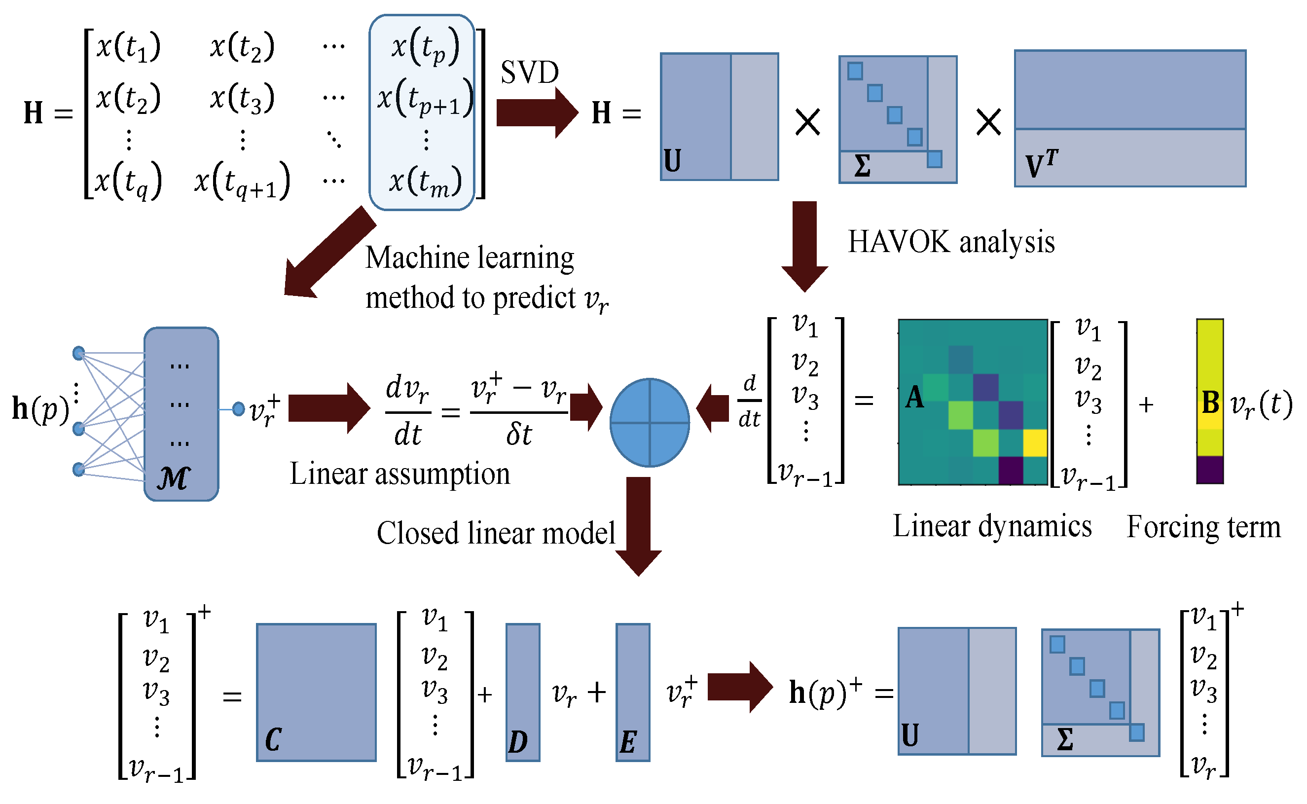
2. HAVOK-ML Method
3. Numerical Experiments
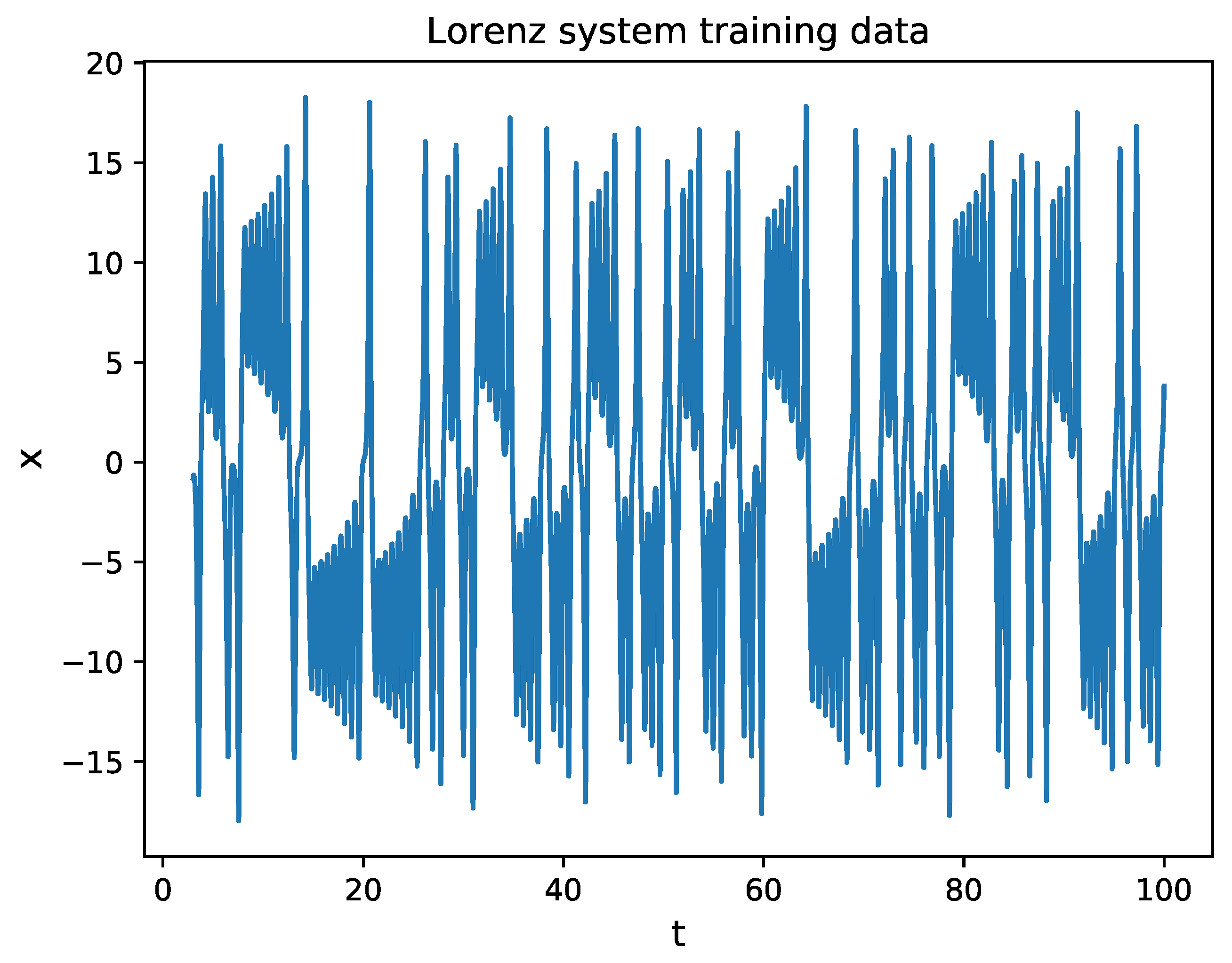
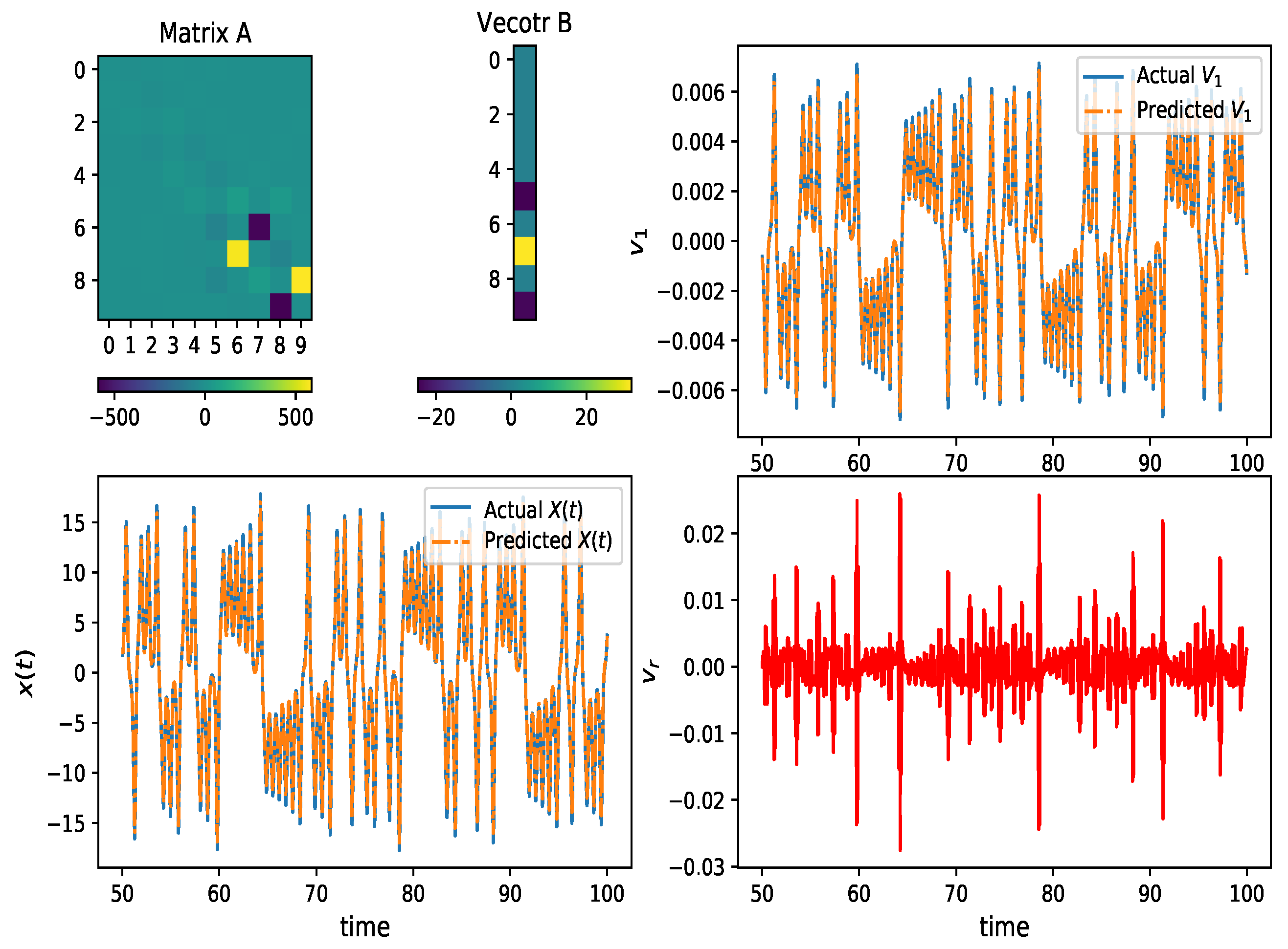
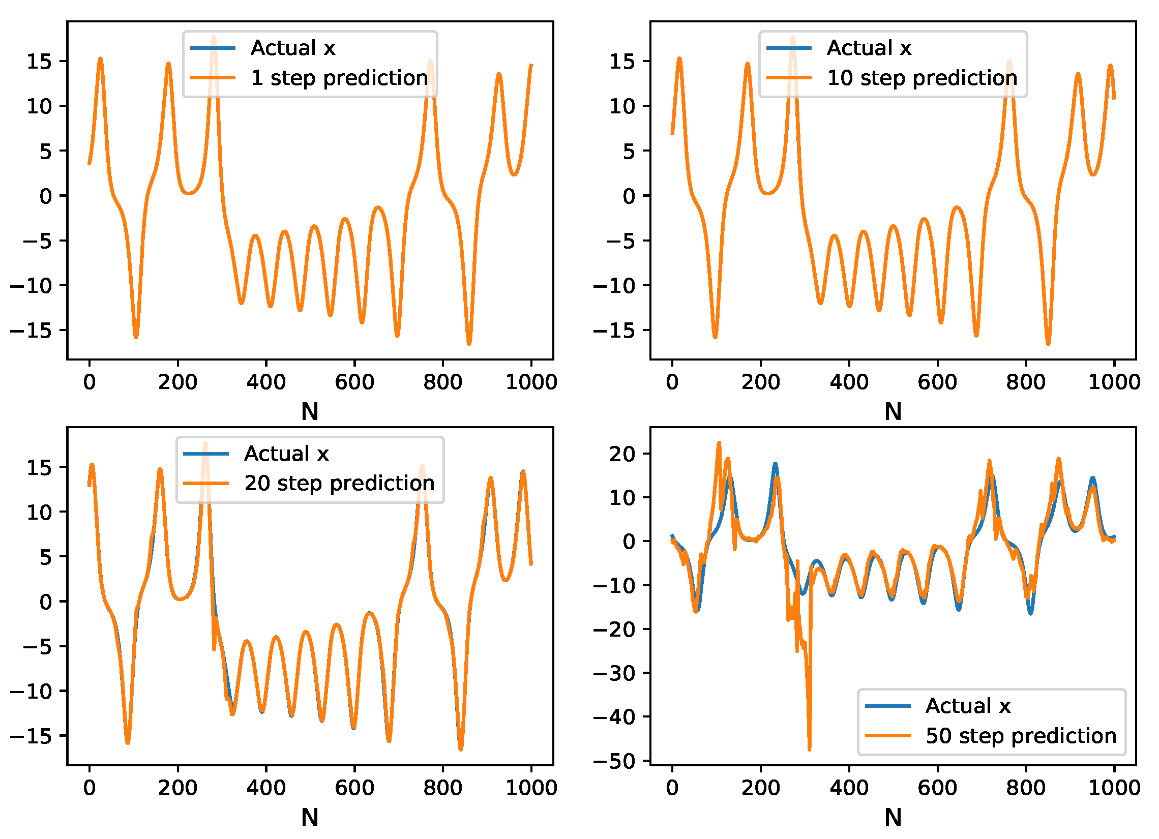
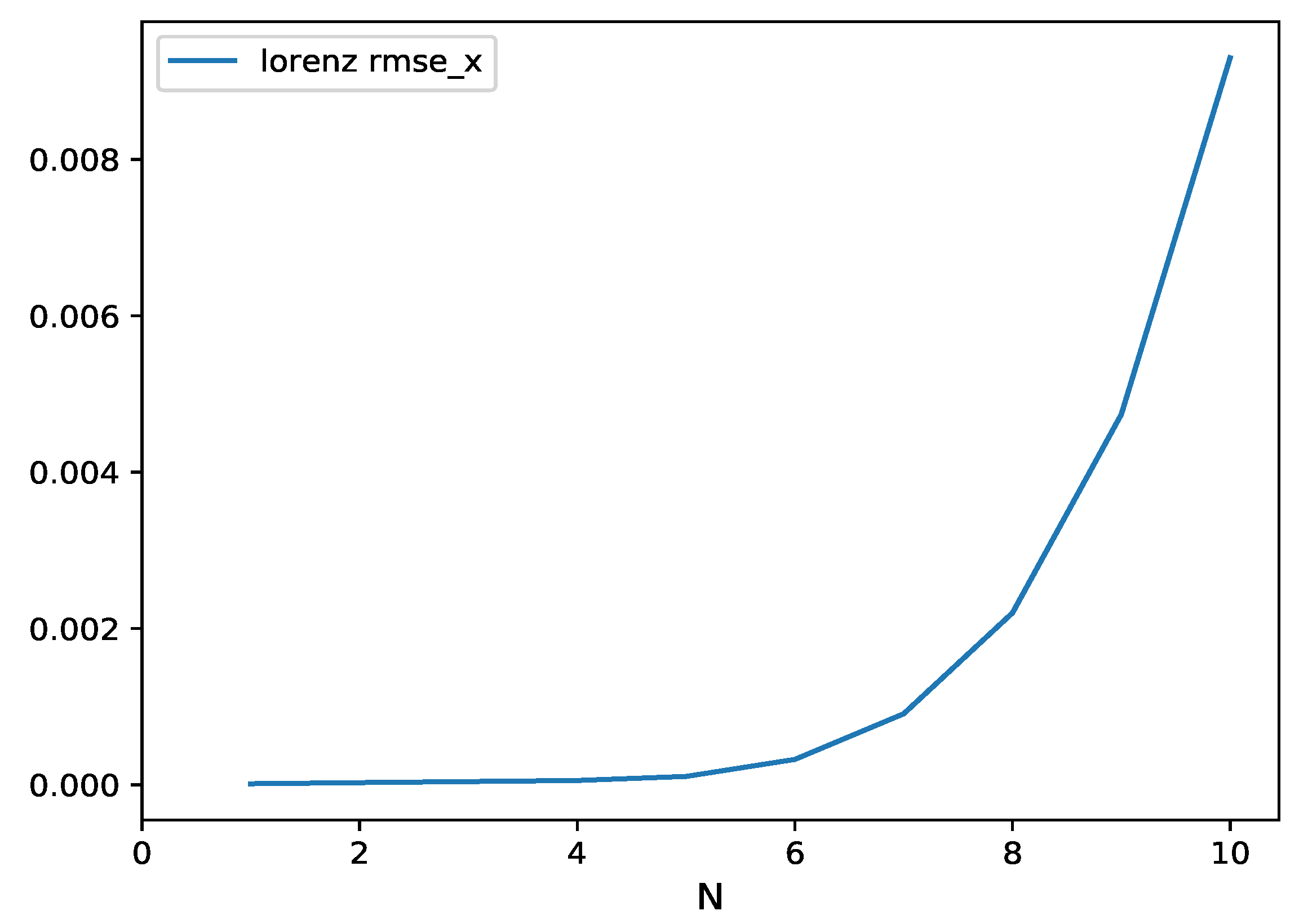
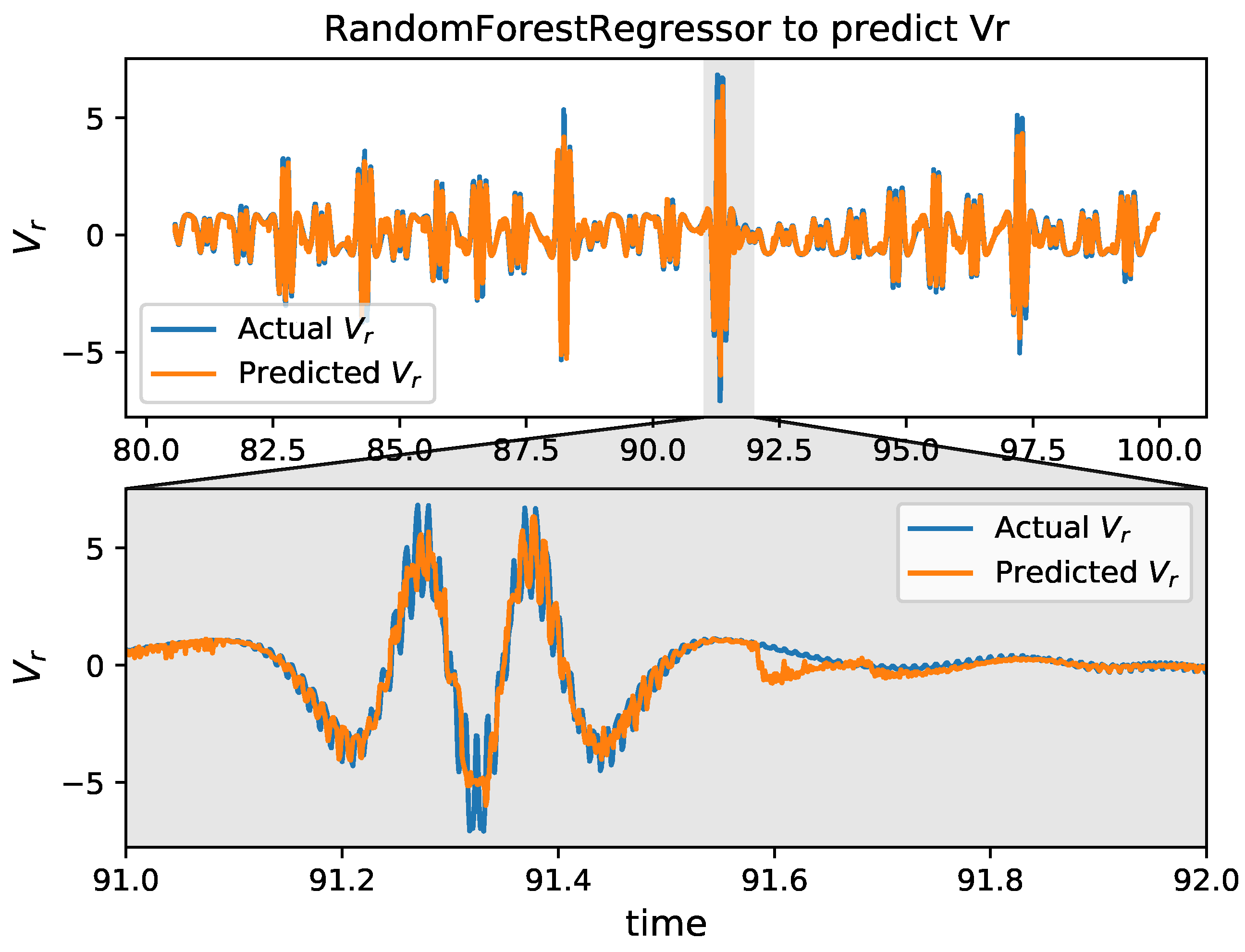
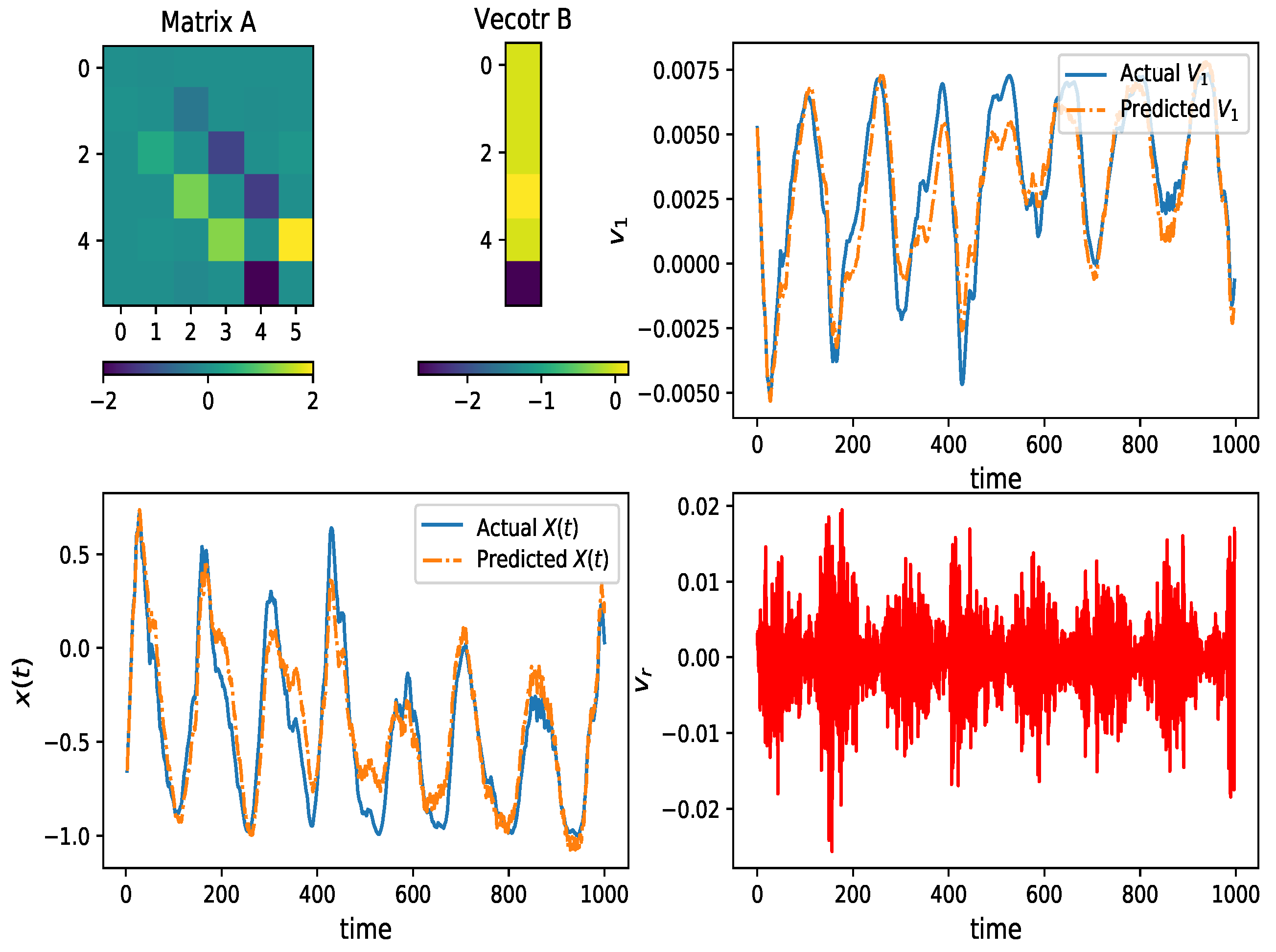
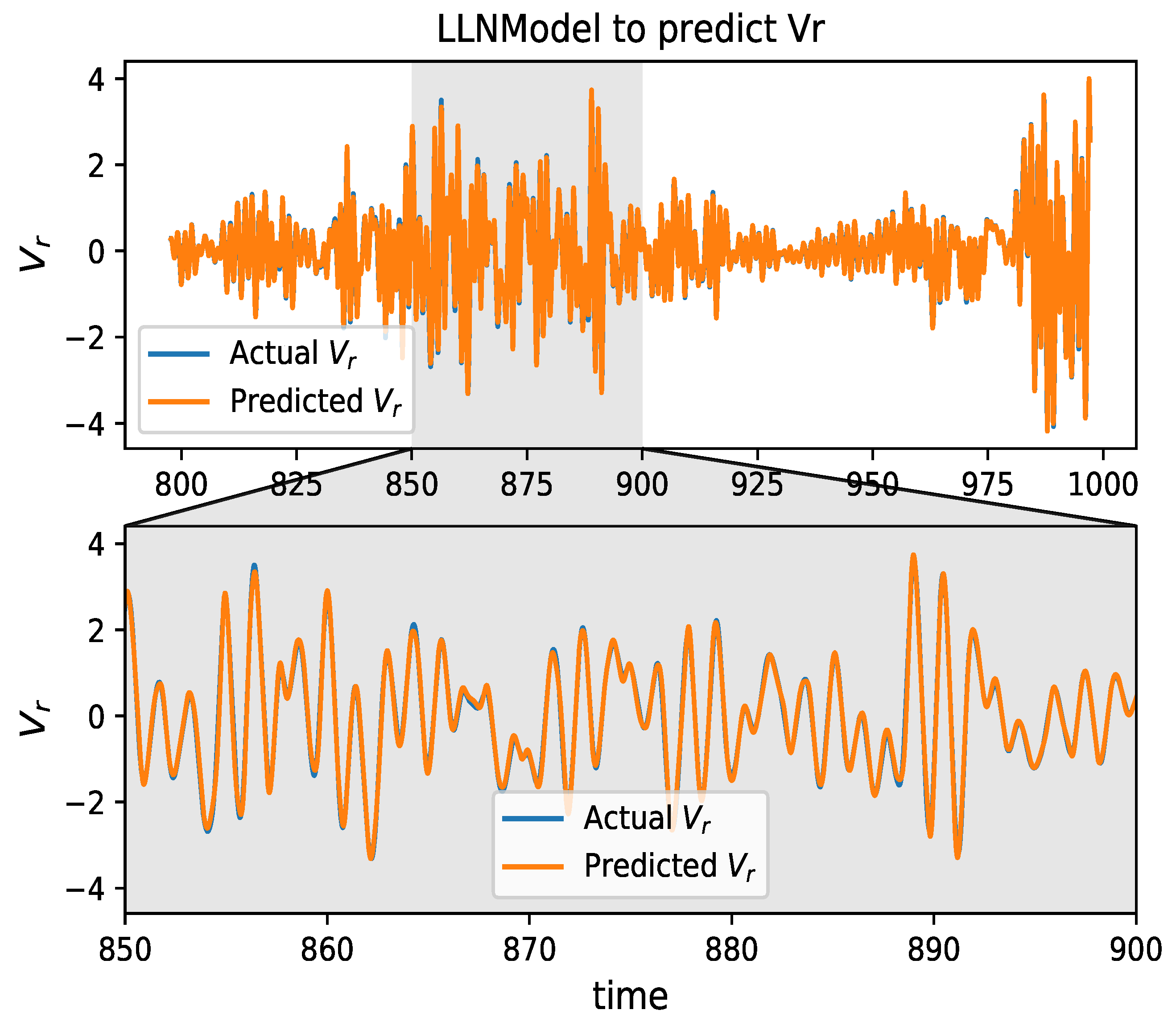
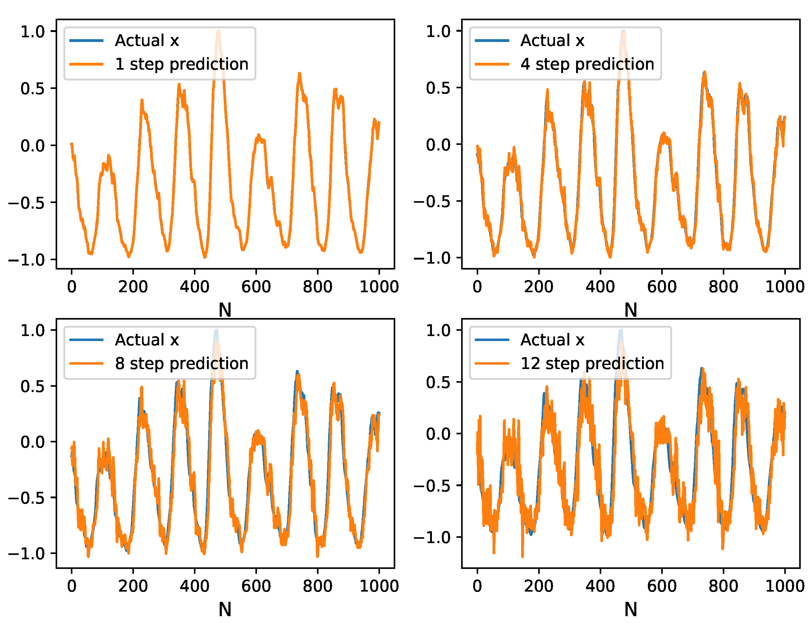
3.1. Lorenz Time Series
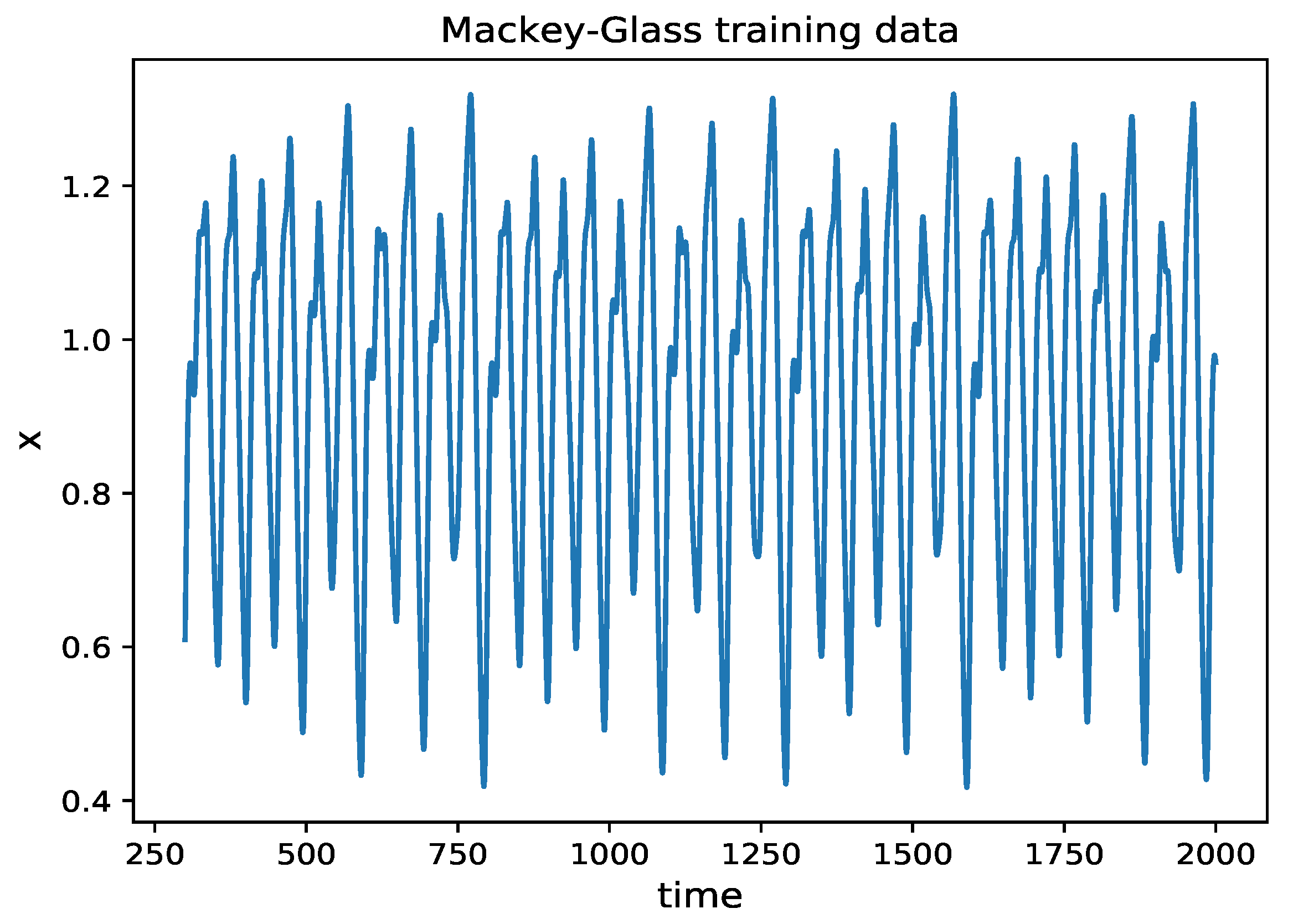
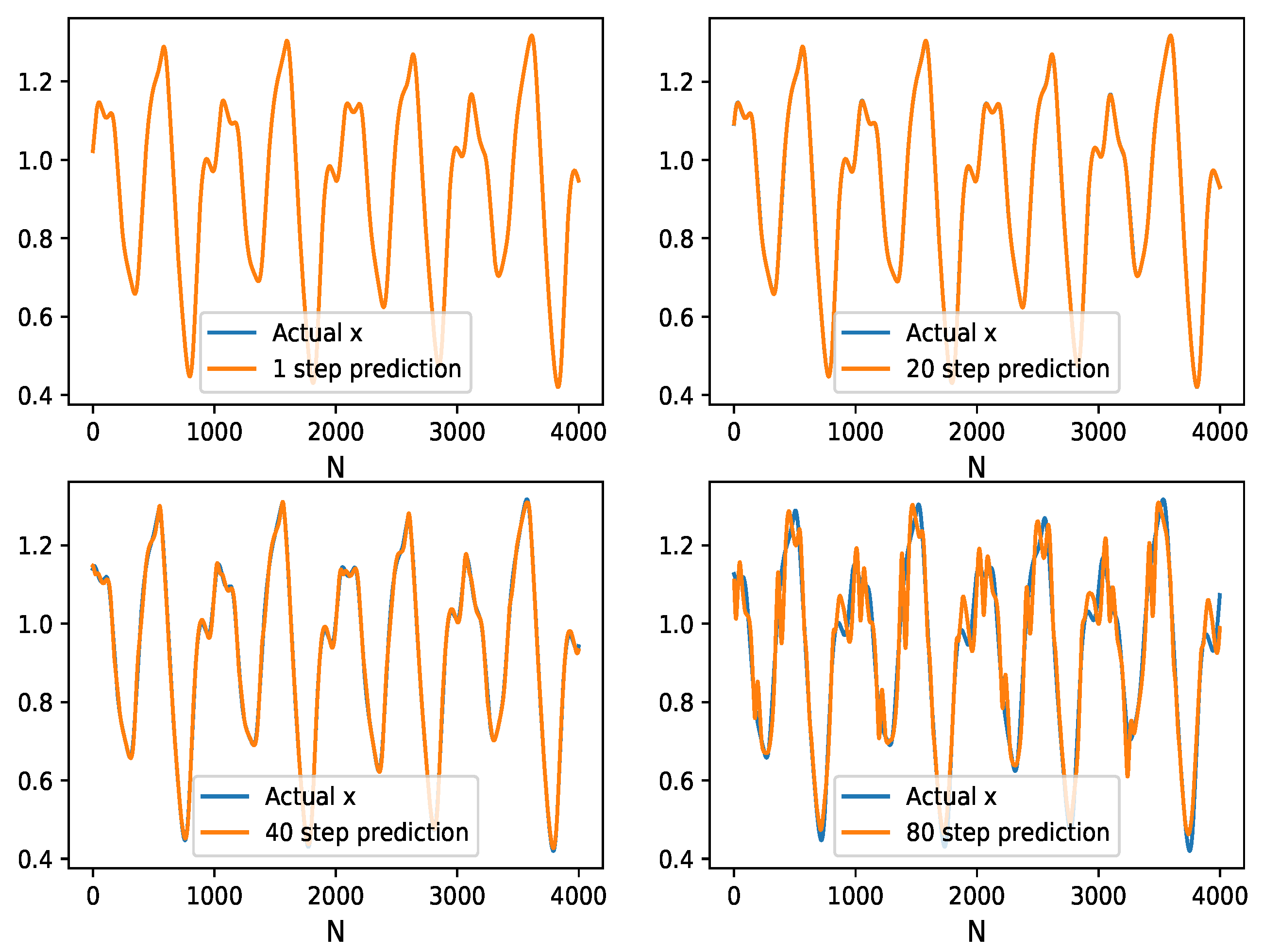
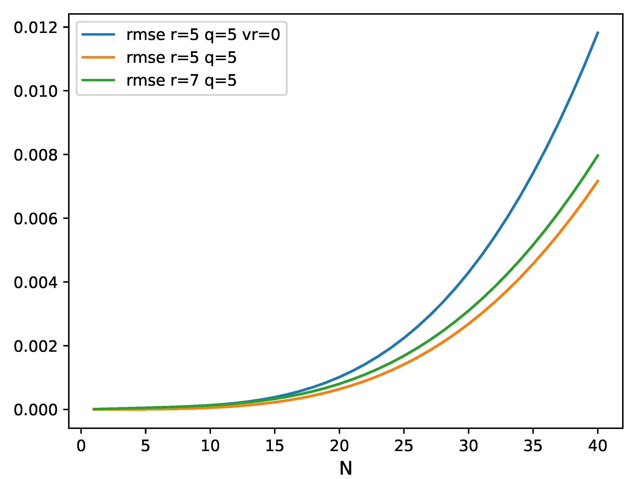
3.2. Mackey–Glass Time Series
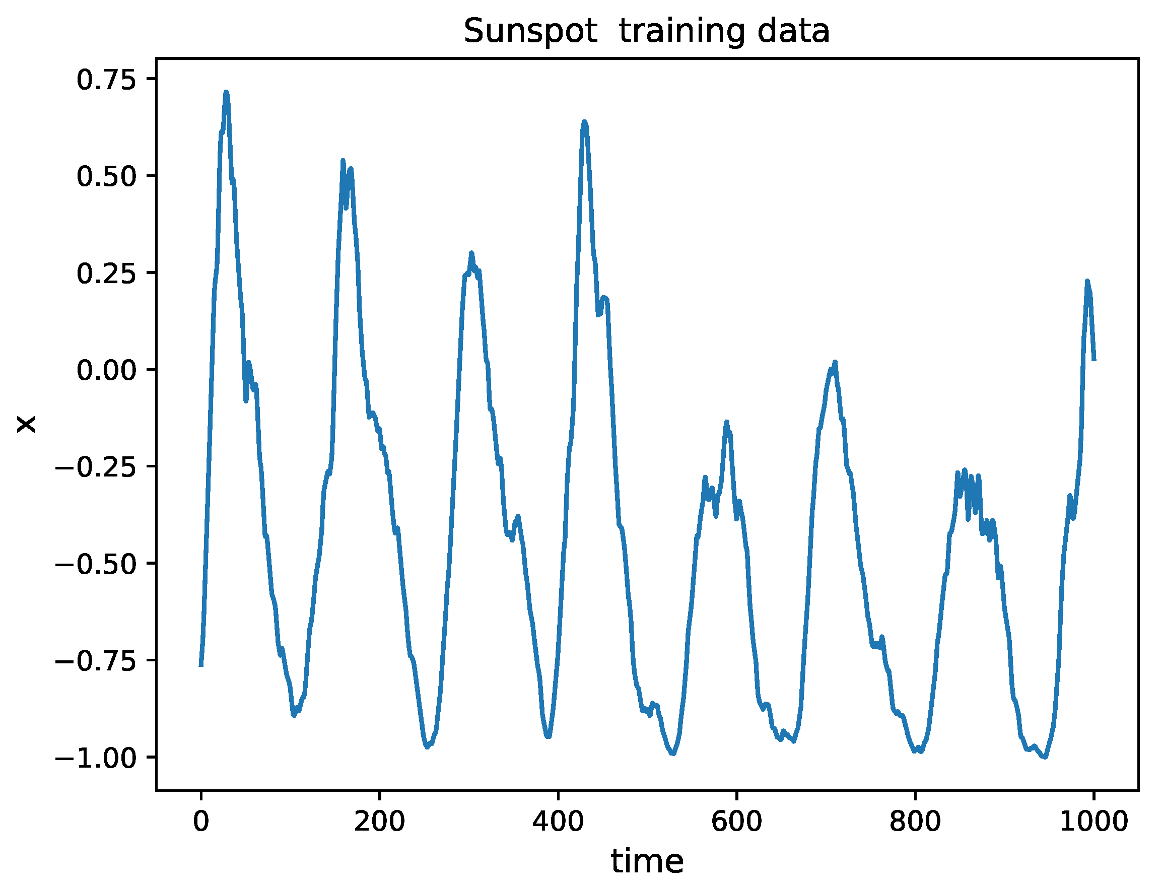
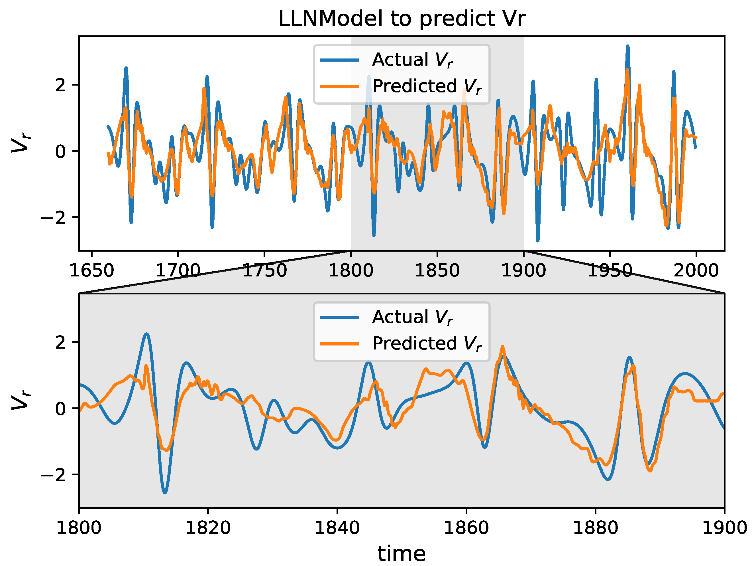
3.3. Sunspot Time Series
4. Discussion and Conclusions
Author Contributions
Funding
Data Availability Statement
Conflicts of Interest
Appendix A. Figures of Mackey–Glass Time Series and Sunspot Time Series


References
- Lorenz, E.N. Deterministic nonperiodic flow. J. Atoms. 1963, 20, 130–141. [Google Scholar] [CrossRef] [Green Version]
- Bjørnstad, O.N.; Grenfell, B.T. Noisy Clockwork: Time Series Analysis of Population Fluctuations in Animals. Science 2001, 293, 638–643. [Google Scholar] [CrossRef] [Green Version]
- Sugihara, G.; May, R.; Ye, H.; Hsieh, C.H.; Deyle, E.; Fogarty, M.; Munch, S. Detecting Causality in Complex Ecosystems. Science 2012, 338, 496–500. [Google Scholar] [CrossRef]
- Ye, H.; Beamish, R.J.; Glaser, S.M.; Grant, S.; Hsieh, C.H.; Richards, L.J.; Schnute, J.T.; Sugihara, G. Equation-free mechanistic ecosystem forecasting using empirical dynamic modeling. Proc. Natl. Acad. Sci. USA 2015, 112, E1569. [Google Scholar] [CrossRef] [Green Version]
- Sugihara, G.; May, R.M. Nonlinear forecasting as a way of distinguishing chaos from measurement error in time series. Nature 1990, 344, 734–741. [Google Scholar] [CrossRef]
- Chen, S.; Cowan, C.; Grant, P. Orthogonal least squares learning algorithm for radial basis function networks. IEEE Trans. Neural Netw. 1991, 2, 302–309. [Google Scholar] [CrossRef] [Green Version]
- Predicting Chaotic time series using neural and neurofuzzy models: A comparative study. Neural Process. Lett. 2006, 24, 217–239. [CrossRef]
- Chen, Y.; Yang, B.; Dong, J.; Abraham, A. Time-series forecasting using flexible neural tree model. Inf. Sci. 2005, 174, 219–235. [Google Scholar] [CrossRef]
- Chandra, R.; Zhang, M. Cooperative coevolution of Elman recurrent neural networks for chaotic time series prediction. Neurocomputing 2012, 86, 116–123. [Google Scholar] [CrossRef]
- Ma, Q.L.; Zheng, Q.L.; Peng, H.; Zhong, T.W.; Xu, L.Q. Chaotic Time Series Prediction Based on Evolving Recurrent Neural Networks. In Proceedings of the 2007 International Conference on Machine Learning and Cybernetics, Hong Kong, China, 19–22 August 2007; Volume 6, pp. 3496–3500. [Google Scholar] [CrossRef]
- Koskela, T.; Lehtokangas, M.; Saarinen, J.; Kaski, K. Time Series Prediction with Multilayer Perceptron, FIR and Elman Neural Networks. In Proceedings of the World Congress on Neural Networks; INNS Press: San Diego, CA, USA, 1996; pp. 491–496. [Google Scholar]
- Kuremoto, T.; Kimura, S.; Kobayashi, K.; Obayashi, M. Time series forecasting using a deep belief network with restricted Boltzmann machines. Neurocomputing 2014, 137, 47–56. [Google Scholar] [CrossRef]
- Ardalani-Farsa, M.; Zolfaghari, S. Chaotic time series prediction with residual analysis method using hybrid Elman–NARX neural networks. Neurocomputing 2010, 73, 2540–2553. [Google Scholar] [CrossRef]
- Brunton, S.L.; Brunton, B.W.; Proctor, J.L.; Kaiser, E.; Kutz, J.N. Chaos as an Intermittently Forced Linear System. Nat. Commun. 2016, 8, 19. [Google Scholar] [CrossRef]
- Inoussa, G.; Peng, H.; Wu, J. Nonlinear time series modeling and prediction using functional weights wavelet neural network-based state-dependent AR model. Neurocomputing 2012, 86, 59–74. [Google Scholar] [CrossRef]
- Zhu, L.; Wang, Y.; Fan, Q. MODWT-ARMA model for time series prediction. Appl. Math. Model. 2014, 38, 1859–1865. [Google Scholar] [CrossRef]
- Ong, P.; Zainuddin, Z. Optimizing wavelet neural networks using modified cuckoo search for multi-step ahead chaotic time series prediction. Appl. Soft Comput. J. 2019, 80, 374–386. [Google Scholar] [CrossRef]
- Wang, X.; Ma, L.; Wang, B.; Wang, T. A hybrid optimization-based recurrent neural network for real-time data prediction. Neurocomputing 2013, 120, 547–559. [Google Scholar] [CrossRef]
- Bhardwaj, S.; Srivastava, S.; Gupta, J.R.P. Pattern-Similarity-Based Model for Time Series Prediction. Comput. Intell. 2015, 31, 106–131. [Google Scholar] [CrossRef]
- Smith, C.; Jin, Y. Evolutionary multi-objective generation of recurrent neural network ensembles for time series prediction. Neurocomputing 2014, 143, 302–311. [Google Scholar] [CrossRef] [Green Version]
- Ho, D.T.; Garibaldi, J.M. Context-Dependent Fuzzy Systems With Application to Time-Series Prediction. IEEE Trans. Fuzzy Syst. Publ. IEEE Neural Netw. Counc. 2014, 22, 778–790. [Google Scholar] [CrossRef]
- Takens, F. Detecting strange attractors in turbulence. In Dynamical Systems and Turbulence, Warwick 1980; Rand, D., Young, L.S., Eds.; Springer: Berlin/Heidelberg, Germany, 1981; pp. 366–381. [Google Scholar]
- Tu, J.H.; Rowley, C.W.; Luchtenburg, D.M.; Brunton, S.L.; Kutz, J.N. On dynamic mode decomposition: Theory and applications. J. Comput. Dyn. 2014, 1, 391–421. [Google Scholar] [CrossRef] [Green Version]
- Brunton, S.L.; Proctor, J.L.; Kutz, J.N. Discovering governing equations from data: Sparse identification of nonlinear dynamical systems. Proc. Natl. Acad. Sci. USA 2015, 113, 3932. [Google Scholar] [CrossRef] [Green Version]
- Ao, Y.; Li, H.; Zhu, L.; Ali, S.; Yang, Z. The linear random forest algorithm and its advantages in machine learning assisted logging regression modeling. J. Pet. Sci. Eng. 2019, 174, 776–789. [Google Scholar] [CrossRef]
- Mackey, M.C.; Glass, L. Oscillation and Chaos in Physiological Control Systems. Science 1977, 197, 287–289. [Google Scholar] [CrossRef]
- Gan, M.; Peng, H.; Peng, X.; Chen, X.; Inoussa, G. A locally linear RBF network-based state-dependent AR model for nonlinear time series modeling. Inf. Sci. 2010, 180, 4370–4383. [Google Scholar] [CrossRef]
- Ganjefar, S.; Tofighi, M. Optimization of quantum-inspired neural network using memetic algorithm for function approximation and chaotic time series prediction. Neurocomputing 2018, 291, 175–186. [Google Scholar] [CrossRef]
- Woolley, J.W.; Agarwal, P.K.; Baker, J. Modeling and prediction of chaotic systems with artificial neural networks. Int. J. Numer. Methods Fluids 2010, 63, 989–1004. [Google Scholar] [CrossRef]


| System | Samples | dt | q | Rank (r) | Regressor for | |
|---|---|---|---|---|---|---|
| Lorenz | 20,000 | 0.01 s | 0.001 s | 40 | 11 | RandomForest |
| Mackey-Glass | 50,000 | 0.1 s | / | 5 | 5 | LoLiMoT |
| Sunspot | 2000 | 1 month | 0.02 month | 140 | 7 | LoLiMoT |
| Model | RMSE | NMSE | Reference |
|---|---|---|---|
| Deep Belief Network | 1.02 × 10 | / | [12] |
| Elman–NARX neural networks | 1.08 × 10 | 1.98 × 10 | [13] |
| WNN | / | 9.84 × 10 | [15] |
| Fuzzy Inference System | 3.1 × 10 | / | [19] |
| Local Linear Neural Fuzzy | / | 9.80 × 10 | [7] |
| Local Linear Radial Basis Function Networks | / | 4.53 × 10 | [27] |
| WNNs with MCSA | 8.20 × 10 | 1.22 × 10 | [17] |
| HAVOK_ML(RFR) | 1.43 × 10 | 3.23 × 10 |
| Model | RMSE | NMSE | Reference |
|---|---|---|---|
| ARMA with Maximal Overlap Discrete Wavelet Transform | / | 5.3373 × 10 | [16] |
| Ensembles of Recurrent Neural Network | 7.533 × 10 | 8.29 × 10 | [20] |
| Quantum-Inspired Neural Network | 9.70 × 10 | / | [28] |
| Recurrent Neural Network | 6.25 × 10 | / | [18] |
| Type-1 Fuzzy System | 4.8 × 10 | / | [21] |
| Fuzzy Inference System | 7.1 × 10 | / | [19] |
| WNNs with MCSA | 5.60 × 10 | 6.25 × 10 | [17] |
| HAVOK_ML(RFR) | 9.92 × 10 | 1.86 × 10 |
| Model | RMSE | NMSE | Reference |
|---|---|---|---|
| Elman-NARX Neural Networks | 1.19 × 10 | 5.90 × 10 | [13] |
| Elman Recurrent Neural Networks | 5.58 × 10 | 1.92 × 10 | [29] |
| Ensembles of Recurrent Neural Network | 1.52 × 10 | 9.64 × 10 | [20] |
| Fuzzy Inference System | 1.18 × 10 | 5.32 × 10 | [19] |
| Functional Weights WNNs State Dependent Autoregressive Model | 1.12 × 10 | 5.24 × 10 | [21] |
| WNNs with MCSA | 1.13 × 10 | 5.30 × 10 | [17] |
| HAVOK_ML(RFR) | 4.25 × 10 | 7.40 × 10 |
Publisher’s Note: MDPI stays neutral with regard to jurisdictional claims in published maps and institutional affiliations. |
© 2022 by the authors. Licensee MDPI, Basel, Switzerland. This article is an open access article distributed under the terms and conditions of the Creative Commons Attribution (CC BY) license (https://creativecommons.org/licenses/by/4.0/).
Share and Cite
Yang, J.; Zhao, J.; Song, J.; Wu, J.; Zhao, C.; Leng, H. A Hybrid Method Using HAVOK Analysis and Machine Learning for Predicting Chaotic Time Series. Entropy 2022, 24, 408. https://doi.org/10.3390/e24030408
Yang J, Zhao J, Song J, Wu J, Zhao C, Leng H. A Hybrid Method Using HAVOK Analysis and Machine Learning for Predicting Chaotic Time Series. Entropy. 2022; 24(3):408. https://doi.org/10.3390/e24030408
Chicago/Turabian StyleYang, Jinhui, Juan Zhao, Junqiang Song, Jianping Wu, Chengwu Zhao, and Hongze Leng. 2022. "A Hybrid Method Using HAVOK Analysis and Machine Learning for Predicting Chaotic Time Series" Entropy 24, no. 3: 408. https://doi.org/10.3390/e24030408
APA StyleYang, J., Zhao, J., Song, J., Wu, J., Zhao, C., & Leng, H. (2022). A Hybrid Method Using HAVOK Analysis and Machine Learning for Predicting Chaotic Time Series. Entropy, 24(3), 408. https://doi.org/10.3390/e24030408