1. Introduction
Cryptocurrencies challenge the validity of modern monetary theory, which says that the legal ordinances supported by a government are necessary to gain the acceptance and trust of a currency by the people [
1]. Bitcoin does not rely on the support of a government, but on its algorithmic design, together with voluntary human users. Bitcoin’s design has shaped both its success and usage. The security of bitcoin stems from voluntary miners maintaining the integrity of the ledger-blockchain [
2]. For extending the blockchain, miners are rewarded with new bitcoins.
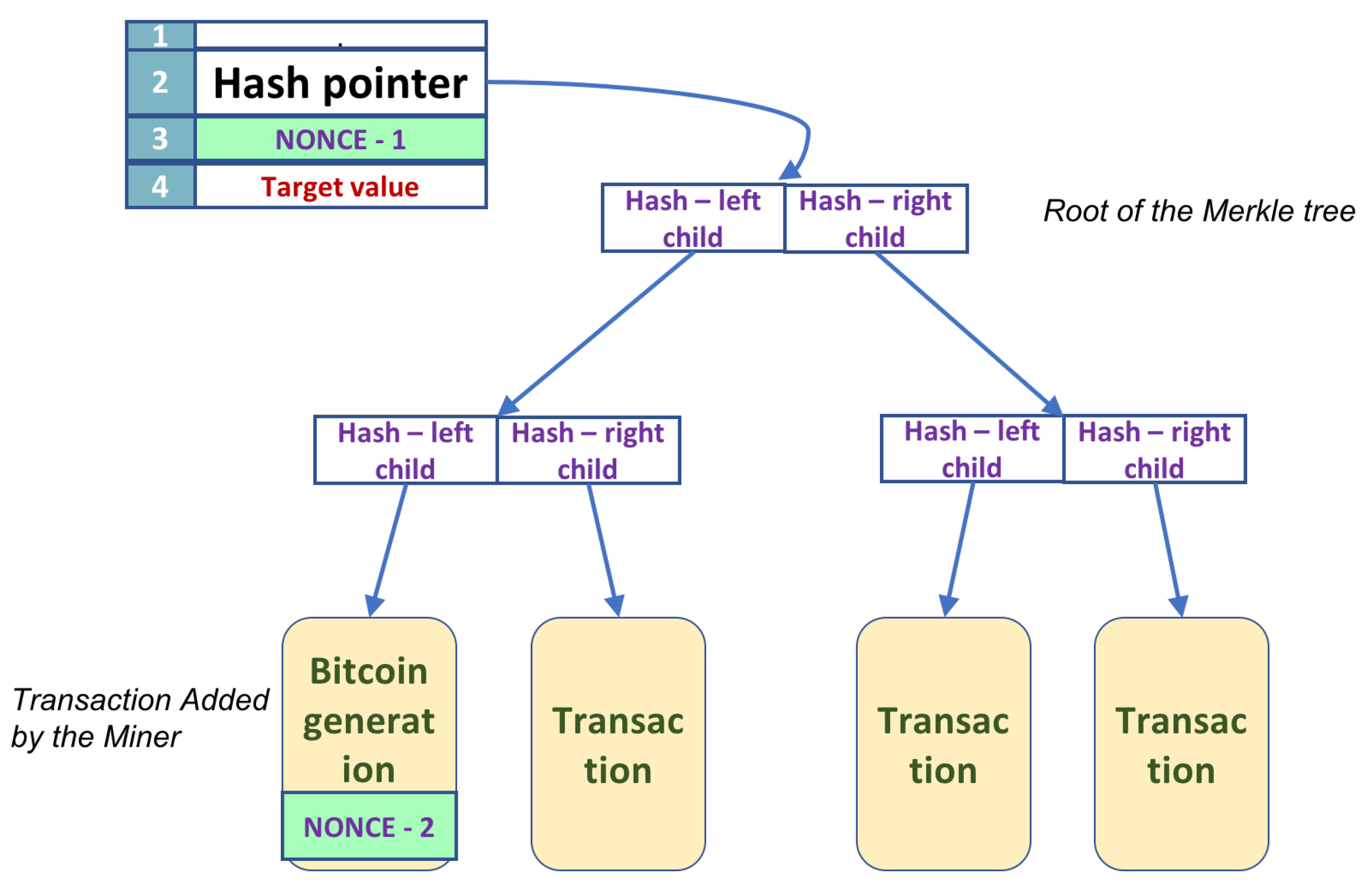
Mining in Bitcoin entails the search of bit strings, called nonces. There are two possible nonces in a block. For a description of the block, consisting of the block header and a Merkle tree data structure, see
Section 3.1. Nonces appear in the block header and in a leaf of the Merkle tree. Golden nonces, or successful nonces, have to satisfy a condition; namely, the hash value of the block header has to fall within a range. Any change to either of the two nonce values affects the value of the overall hash. When the primary nonce in the block header changes, the hash is easily recomputed. In contrast, changes to the extra nonce, in the leaf of the tree, require the recalculation of parts of the Merkle tree, and thus the recalculation of the hash requires a time complexity dependent on the height of the tree.
Bitcoin mining is a lucrative business. There are large companies that specialize in Bitcoin mining operations. The basic algorithmic approach for mining nonces remains the same: search the nonce values space by trying out possible nonces, either in a predetermined order or in some randomized order. By assumption, there is no bias on golden nonces, and therefore all nonce values are equally likely to be successful. A randomized search is, therefore, the best algorithmic strategy available on a classical computer. To speed up the nonces’ search, significant hardware has been developed. There are four generations of Bitcoin mining hardware: the CPUs, collection of GPUs, FPGAs, and ASICs.
The advantage of using a quantum computer for nonce mining has not been studied exhaustively. Previous studies have assumed that the difficulty of re-hashing remains the same even when the nonce in the Merkle tree is updated [
3]. This paper contributes to this direction with a quantum algorithm that uses quantum parallelism to check all possible nonces in superposition at once. The algorithm improves the previous work by utilizing quantum unstructured search to search for the extra nonce, which is more costly. Therefore, the size of the extra nonce and the size of the search space is the miner’s decision. In the quantum algorithm proposed here, the Merkle tree is walked through only once. Additionally, the use of Grover’s search algorithm adds to the search’s complexity, a term on the order of
, where
N is the size of the search space. This is a theoretical, algorithmic change that speeds up the nonce’s search by a quadratic factor. Present-day quantum computers are far from a physical realization of the algorithm presented here; the restrictions are as follows:
The number of qubits is low.
The gates and transformations implemented is restricted to the number of inputs and outputs.
The circuit size is limited in depth and breadth.
Nevertheless, well-sized quantum computers would consistently outperform classical hardware in search of golden nonces.
The rest of the paper is organized as follows.
Section 2 shows previous connections between Bitcoin and quantum cryptography/computation, both as a threat and also some solutions.
Section 3 briefly describes the necessary data structures and mining procedures for Bitcoin.
The quantum mining algorithm is described in
Section 4. The algorithm has five steps that follow the logical flow of the mining process. Most of these steps rely on both classical and quantum information. The quantum computer’s size and the algorithm’s time cost are analyzed in
Section 5. A comparative discussion on the implication of quantum mining in Bitcoin, i.e., quantum supremacy, is discussed in
Section 5. Quantum computers are considered to bring about the end of current security systems and solve the problem of security better with quantum security systems.
Section 6 concludes the paper.
4. Quantum Algorithm for Bitcoin Mining
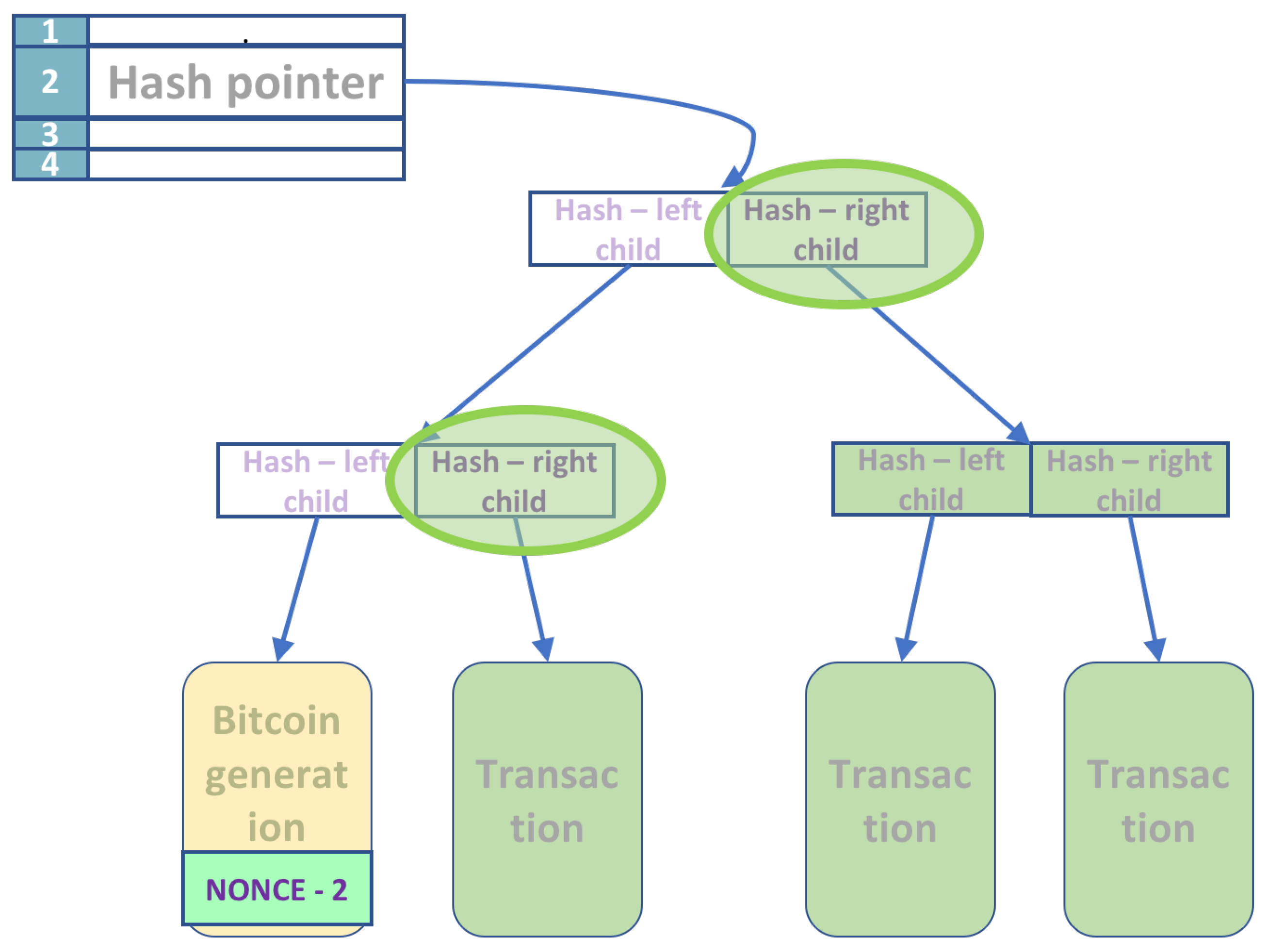
The only possibility to generate new bitcoins is by participating in the maintenance of the Blockchain, the history of all transactions, which keeps the currency alive. Mining involves searching for the two nonces (header and the extra nonce), such that the Hash of the block header is below the target specified. (
Figure 3)
We suppose that we have a quantum computer with sufficient qubits to perform all the operations. We will separate the classical part of the circuit needed to compute the permanent part of the Merkle tree and for the application of SHA-256. This separation yields a hybrid solution; the quantum computer needs fewer qubits and works together with a classical computer. There are five stages, and the circuit description for each stage is next.
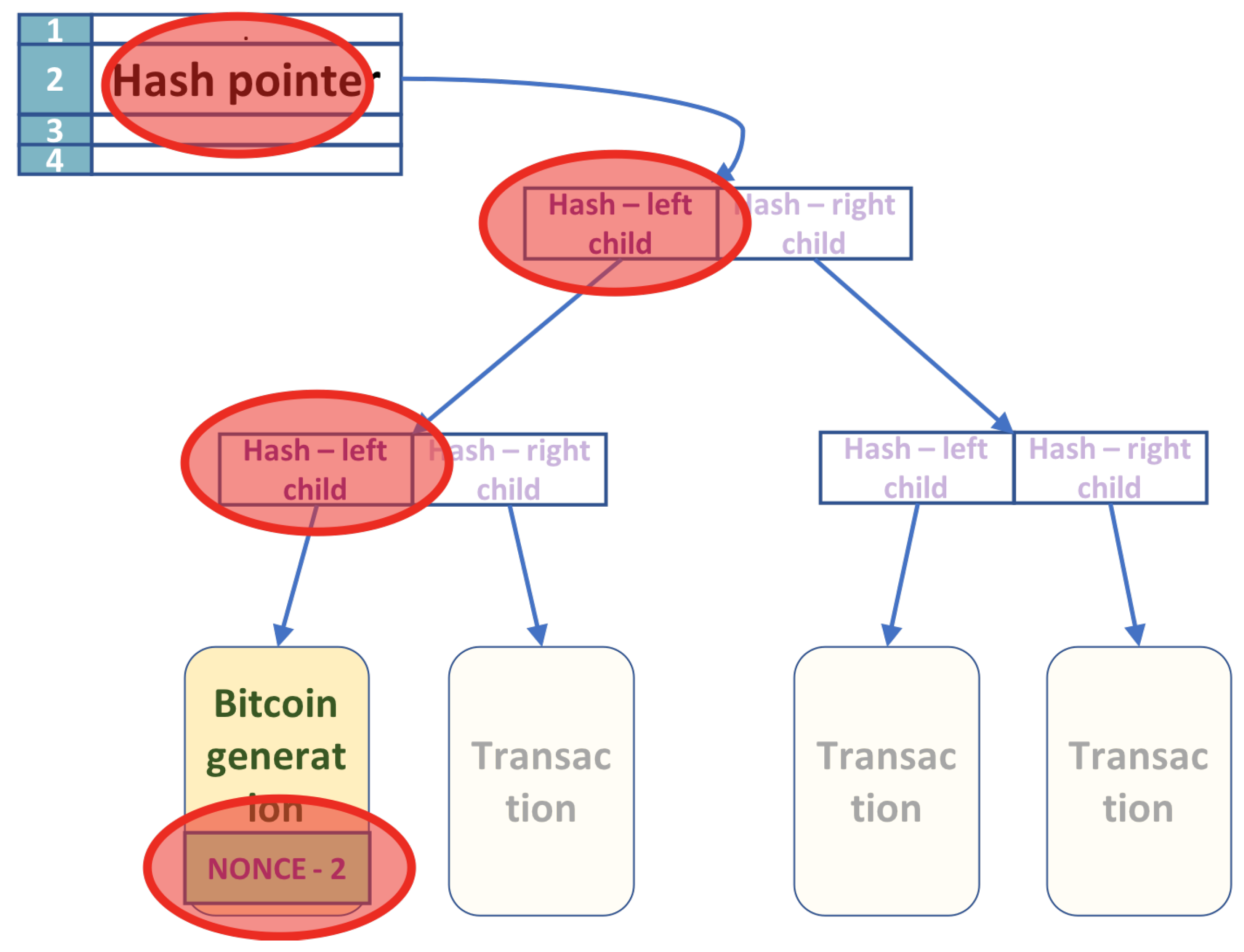
The algorithm computes all the permanent values at the start and only once. As shown in
Section 3.1, whenever the nonces change values, only a few nodes in the Merkle tree change. Consider the tree shown in
Figure 2. The tree has
n leaves, with transactions in leaves ordered from left to right
,
, …,
. The first leaf
contains the nonce, but the other transactions are permanent. The fields affected by the change of the nonces are marked with a red circle.
Given the transactions in the tree, we compute classically, using post-order traversal, all the hashes at intermediate nodes that they determine. The result of this step is an array of size at most n that contains all the right hashes in the Merkle tree, including the ones on the leftmost path. The left-hashes on the Merkle tree’s leftmost path are computed using a quantum algorithm that will be described later.
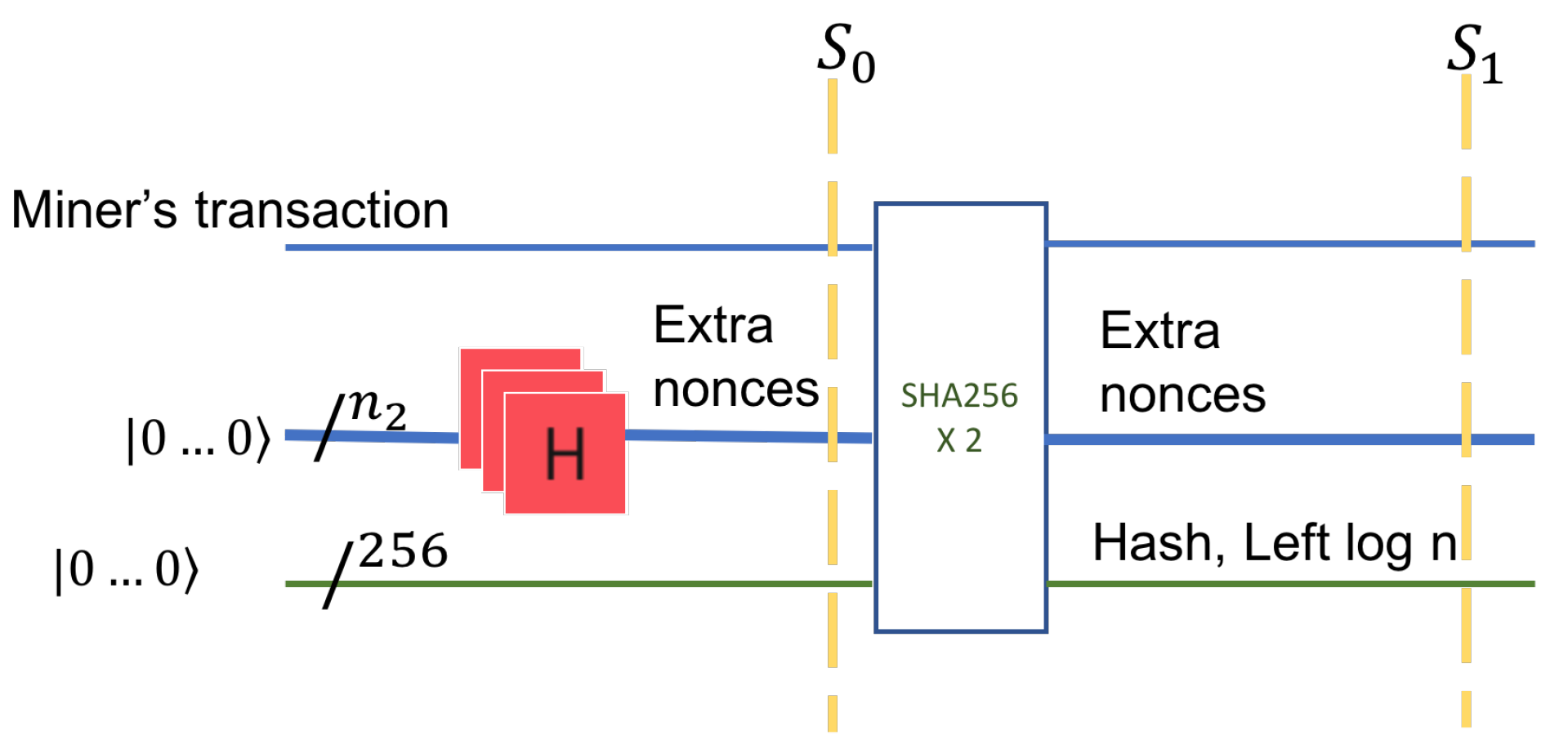
The hash function used by Bitcoin (HASH) is the double application of SHA-256. Each non-leaf node stores the concatenated Hash of its children. All the hash values computed as above are used in Step 3. We know the left and the right hash for every non-leaf node that does not lie on the leftmost path. For nodes that are on the leftmost path, we know only the value of the right hash. The hash values are computed using a post-order traversal, and the time it takes is proportional to the size of the Merkle tree ().
The next step is to compute the hash values at the parent of the leaf , containing the nonce. This hash value is computed using a sequence of quantum circuits, as shown next.
In the first stage, we prepare the input to the quantum circuit. We treat each state as equally likely and consider a superposition of all the states. The number of bits in extra nonce is
. A quantum register of size
, that is a uniform superposition of all possible binary values, is prepared. This is accomplished with an application of
Hadamard gates applied to a register with value zero, as shown in
Figure 4, on the first horizontal line.
In the second stage, we consider the data in leaf
. The nonce register is concatenated to a possibly classical register (
) that holds the miner’s transaction data. The miner’s data refers to the miner’s Bitcoin identity, the address, and the value in bitcoins rewarded for the block creation. This data is classical yet inputs into a quantum circuit. After concatenation of two registers, the set of all possible states is shown by tensor product, denoted by ⊗. The circuit in
Figure 4 has 256 additional input qubits. These inputs have the value
on the left (input) side of the circuit and will carry the value of the HASH on the right side of the circuit, the output.
The input remains unchanged in the output. HASH itself has a quantum implementation [
22]; however, in our later analysis, we consider a classical circuit for HASH.
The third stage is the application of the function HASH. HASH allows input of an arbitrary size but always outputs 256 bits. This circuit has constant depth [
20].
The input after the application of the Hadamard gates is
The output (
) of this state is an entanglement of the extra nonces, the miner’s transaction in
, and the hashes of all nonces. If we denote by
the hash value at the parent of
, then the state of the quantum system after the application of HASH is
The next step computes the remaining hashes on the leftmost path in the Merkle tree.
The hash values are computed sequentially in a bottom-up fashion. Instead of computing the hash values at each node for every nonce input sequentially, we again rely on quantum parallelism. With a single application of a quantum circuit, we compute in parallel all the hash values for all possible nonce inputs at a given node. The number of such stages is proportional to the number of nodes in the leftmost path.
The initial input is part of the entangled superposition
, which is concatenated with the right-hash of the internal node at level
. This right-hash is already computed in Step 1. HASH is applied to this input. A 256 qubit register (initialized to 0) is used for the output. This circuit is again guaranteed to exist, as discussed in
Section 3.2.
Figure 5 shows the operation in the first stage on the left. From here on, the hash output of the previous level is the input to the HASH circuit of the next level (as the Hash of the left child). Each sequential circuit has the same three inputs: the hash of the previous level, the hash of the right child, and a register of 256 zeroes to hold the result. After
levels, the hash of the Merkle tree root is the output. The output is in a superposition state, and for every state (nonce value)
s, we have HASH(
s). Note that at each level, some qubits are discarded.
The useful part of the output is the initial superposition of all nonces and the superposition of all HASH(s) at the root of the Merkle tree, shown in green in
Figure 5. We denote this useful output by
. After this state, the complete state of the system,
, is an entanglement of all useful and non-useful qubits.
can be described only by a density matrix, obtained from
after tracing out the unused qubits. Using the notation in [
18] for a subsystem, we have
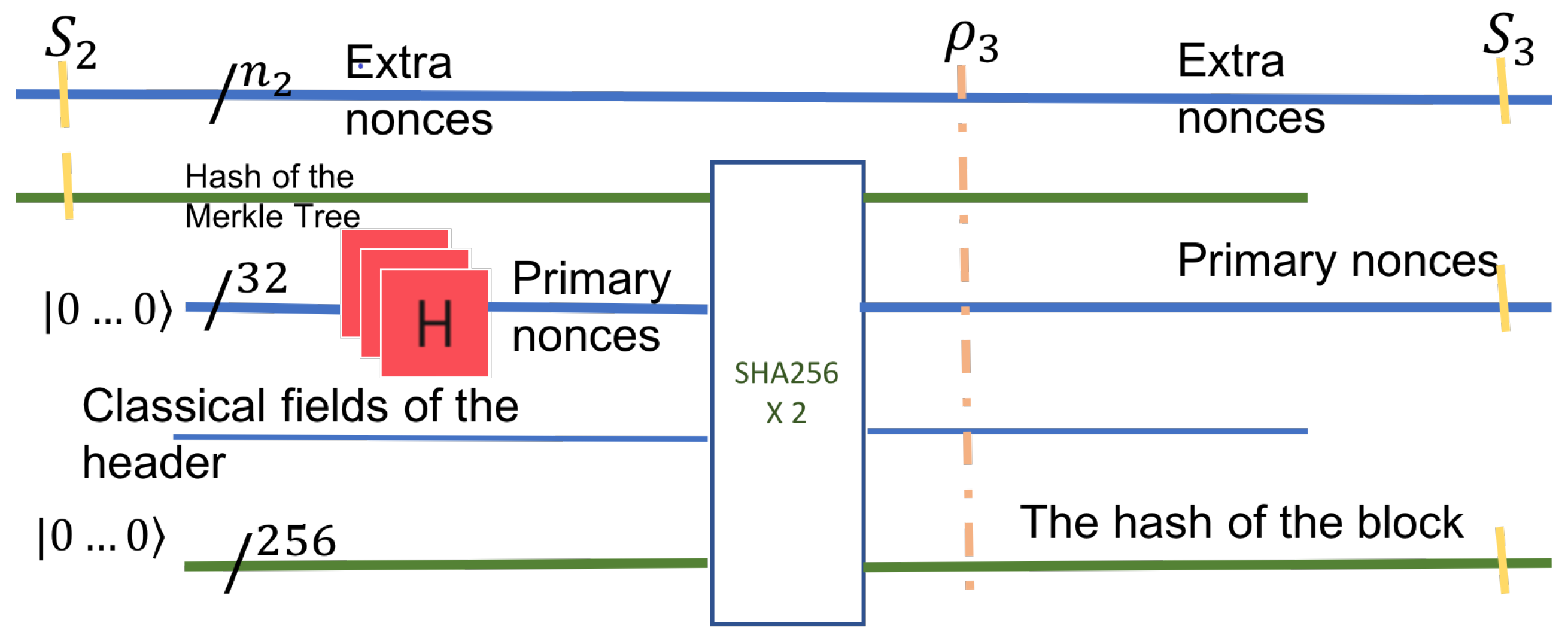
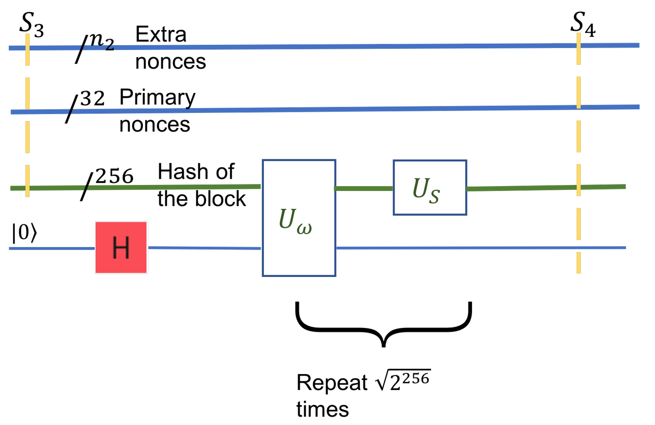
The next step computes the hash of the 4-tuple, given the nonce in the block header. The subsequent step is the use of Grover’s algorithm. The final step is the measurement, which identifies the two nonce values with sufficiently high probability (
Figure 6).
This step deals only with information from the block header. It works with two quantum registers in superposition. The first quantum register is the output of the previous step, . The second quantum register is the superposition of all header nonces. The header nonce is of fixed size, 32 bits. Therefore, it can be represented as a 32 qubit register holding all primary nonce values in superposition. The superposition is generated in the usual way with Hadamard gates.
The hash computed in Step 3 is fed into a HASH (SHA-256x2) circuit and the rest of the header fields. This step is a milestone of the quantum computation as it now has all the possible hash values in a single 256 qubit quantum register. This step’s useful output is an entangled superposition of three quantum registers: all possible hashes, together with the primary nonces of the header, and the extra nonces from the leaf of the Merkle tree. This state can be described as a mixed state of the entire system. If the system at this stage is denoted
, then the useful output
is the mixed state of the three quantum registers after the unused qubits have been traced out.
The input to this step is the hashes’ entire search space in the block header. In , every pair of the primary nonce with the secondary nonce is entangled with the block’s hash.
In particular, the size of the search space is given by the three registers: the header-nonce is of size 32, the size of the extra nonce, , and the block-hash is of size 256. The hash’s size does not contribute to the search space, as it is dependent on the nonces. The two types of nonces are independent and thus define the search space’s size, which is . The state given by these three registers is mixed but describes the system as seen by the Grover circuit in this step,
Most of the components in the state
do not contain the golden nonce. However, there is at least one golden nonce among them, extracted by Grover’s algorithm, with a sufficiently large probability. Grover’s algorithm enhances the probability of the solution. Otherwise, from a uniform superposition of the entire search space, the solutions’ coefficients become arbitrarily larger than those of the non-solutions. We define a conditional NOT inversion operator
that inverts only components that represent a solution. This operator acts on the block hash
, together with an ancilla qubit. The ancilla qubit is a boolean value that will hold a superposition, one for a solution, and zero otherwise, see
Figure 7. The transformation
, the reflection operator, acts as a definite increase to the solution’s amplitude and reduces the amplitude of the non-solution components. These two transformations are applied iteratively for
times, where
is the number of solutions combined and is the probability of all solutions to approach 1.
The state after this step, the resulting state of the system, is . It is similar to in structure, and the amplitudes of the solutions are larger in magnitude (arbitrarily close to 1).
The final step is to measure the qubit registers to determine the header nonce’s value and the extra nonce. The measurement collapses the state, and we get classical information back. As Grover’s algorithm has amplified the states’ amplitudes that correspond to a solution, a measurement will collapse the system to a solution with high probability. As in all quantum algorithms, only one solution can be extracted. The others will be forever forgotten after the collapse. Several repetitions of the quantum algorithm can be performed to boost the classical probability of success. The state after this step will be
where + denotes concatenation of strings. Note that the last 1 denotes the success of the findings. In the unlikely case where the last bit is 0, it means that the nonces in the result are actually not solutions.
The resulting nonce values can now be tested classically, and they should be good. The header nonce and the leaf nonce are inserted in the new block, and the block is ready for broadcasting to the network peers. This ends the general description of the quantum algorithm for finding the header and the leaf nonce. Let us apply the steps on a small example.
A Small Example
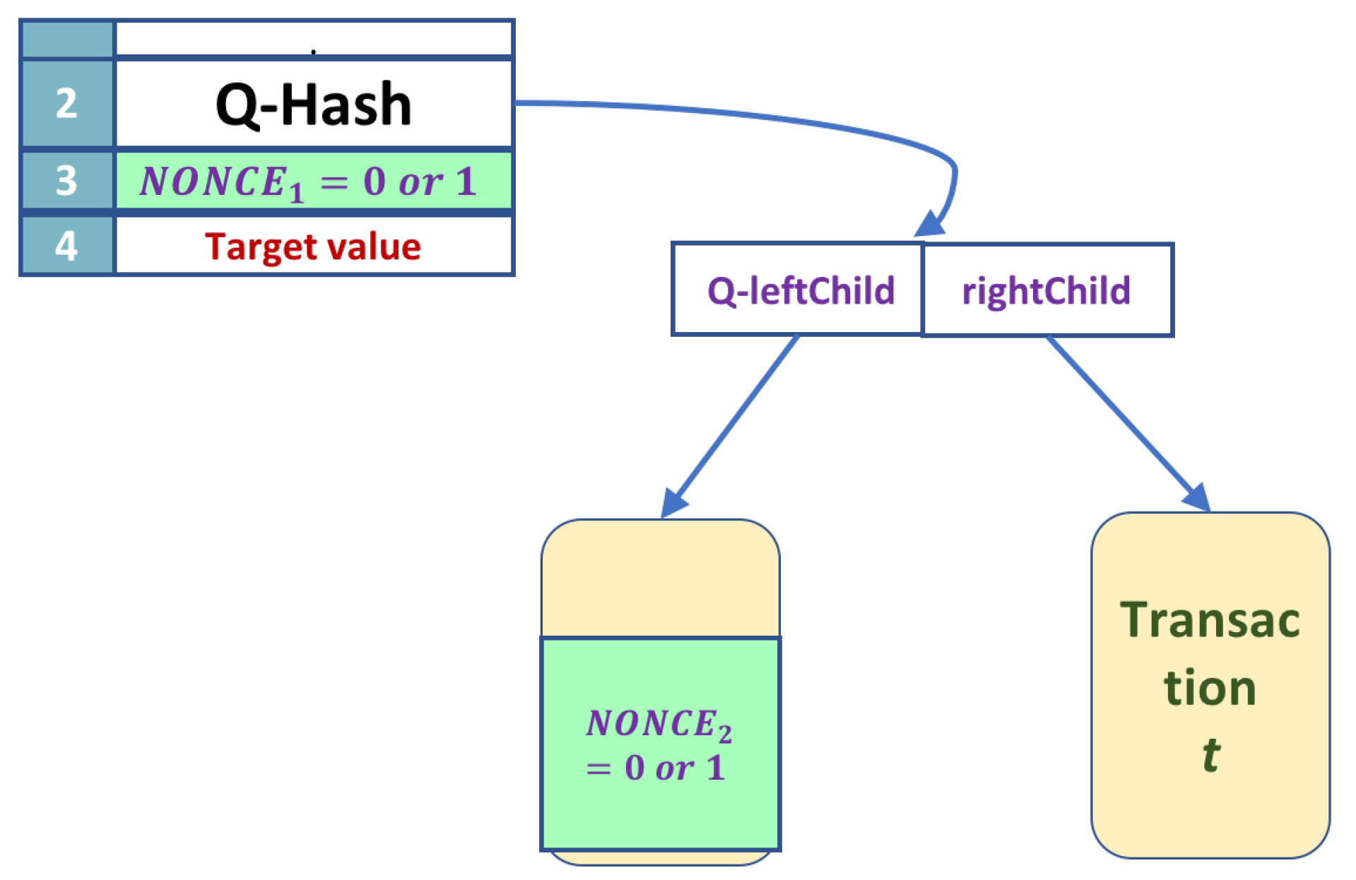
To see how the algorithm is applied, let us consider a small, degenerate example. We will consider the smallest possible Merkle tree and the smallest nonces; see
Figure 8. Let the Merkle tree have two leaves only and let both nonces be of size 1; one qubit. In this case, the nonce search space is of size
, namely
. For definiteness, let us consider that the golden nonce is 01. This value is chosen as a proof of concept and not resulting from any calculation.
The target value in the header is the size of a SHA-256 output, namely 256 bits.
The following transformations show a simplified application of the algorithm’s steps.
The tree has only one transaction
t. This transaction is hashed twice with SHA-256. For simplicity of notation, we will denote
. The computation in this step is
The extra nonce is now prepared in a superposition of all possible values. In our case, with nonces of size one, this is a simple superposition of 0 and 1.
For simplicity, ignore the miner’s transaction. Then, the state
can be written as
In this step, the hash of this leaf is computed:
where
is the quantum transformation that implements SHA-256 twice.
For our example, this step is degenerate, as the height of our tiny tree is one. The new state is the simple concatenation of the output of the previous two steps.
This step computes the final hash. The final hash is applied on the header. The header consists of
The quantum hash of the Merkle tree,
The primary nonce, in superposition of all possible values. This is similar to the initial superposition of the leaf nonce.
Some additional classical information: the target value and some identification information for the block. For simplicity, we denote this information with , and though classical, it needs to be fed into the circuit as quantum values, .
The input to step 4 also contains the qubits for the value of the hash
. The result of this step is obtained as follows:
To get a term by term formula, we rearrange the terms of the superposition.
After applying
, we get:
In the above formula,
represents the application of
on the first term:
, , have similar meanings.
Step 5 applies a standard Grover transformation on
. In order to do this, we need to concatenate
with an ancilla qubit
and then apply Grover transformation, to be denoted here as
G. The result is an amplification of the coefficient of golden nonces.
As the coefficients are probabilities, they obey the condition . Notice that, for the second term, the ancilla qubit is , showing that 01 is the golden nonce. According to Grover, the respective probability coefficient is large, .
In the final step, the state is simply measured and will collapse to one of the terms of the superposition. Because the second term has a large probability coefficient, the state of the system will most likely collapse to
The golden nonce is visible in the first two qubits of the state. Additionally, the ancilla qubit works as a check for the correctness of the nonce.
The question remains: what is the gain in speed or time complexity, realized by this quantum algorithm over the classical algorithm?
5. Size and Cost of the Quantum Solution
The algorithm described in the previous section is a hybrid one. It uses both classical and quantum information. Information such as the customers’ transactions and hash values at the nodes other than the Merkle tree’s leftmost path is all classical information. Nevertheless, the right-hash values (which are classical) along the leftmost path in the Merkle tree do participate in the computation of the hash’s quantum superposition at the root of the tree. Thus, this information has to be fed into a quantum circuit.
Quantum circuits in quantum computers so far explicitly expect qubits as inputs and provide qubits on the output. The output qubits are measured to provide an answer as a binary string. Our analysis will suppose that we have sufficient qubits in the quantum computer to hold the complete input (including the classical information) to quantum circuits.
The primary purpose of developing the quantum algorithm is to outperform classical miners. The search space of the nonces is
. The mining process on a classical computer is memoryless, so the exhaustive randomized search is performed by the miners [
17]. The mining difficulty is a measure of the time that miners need to find a nonce, which, on average, is about 10 min for the Bitcoin Blockchain.
The situation with the quantum algorithm is very different because of quantum parallelism. For the classical part of the algorithm, we use the worst-case running time as a measure. For the quantum part, we use the depth of the quantum circuit as a measure of complexity.
- 1.
Step 1. This step is a classical computation on the Merkle tree. Each node is traversed a constant number of times. The nodes on the leftmost leg of the tree are processed in the next steps. The number of leaves is n. Thus, the computation of this step is a classical .
- 2.
Step 2. This step works on one single leaf node (transaction node) with a quantum superposition. It takes constant time, .
- 3.
Step 3. This step computes the superposition of the hash values along the leftmost path of the tree. The tree has levels, and each level takes constant time. The overall execution time for this step is .
- 4.
Step 4. This step computes the superposition of the hash values in the header. The overall execution time for this step is constant, .
- 5.
Step 5. This step is an application of Grover’s algorithm on the superposition of all hashes of the block. As the hash is of length 256 and there are t solutions, this steps takes .
- 6.
Step 6. This step performs a constant time measurement. Additionally, but not necessarily, the step may check the Hash with a classical algorithm. The execution time is a constant, .
The most costly steps in the above algorithm are step 3 and step 5. We can say that the overall complexity of the quantum algorithm is , where n is the number of transactions, 256 is the size of the output of HASH, and t is the number of golden nonces. We may reasonably consider that , the number of transactions, is significantly smaller than the search space of the nonces. Thus, the time complexity becomes . This is a quadratic improvement over the classical complexity discussed next.
A crude estimate of the search space is given by the total size of two nonces,
. If we assume that the header nonce alone is sufficient to provide a right hash, then, as SHA-256 returns a 256-bit output under the standard cryptographic assumptions, the expected number of hashes to be tried is
, where
t is the target or the number of solutions. The difficulty of finding a header nonce classically can be computed from the target value described in
Section 3. If the extra nonce field is also used to determine the nonce values, then the overhead associated with the computation of hash values at the intermediate nodes in the Merkle tree has to be taken into account.
To the best of our knowledge, no analysis of difficulty (either classically or quantumly) addresses this. Ours is the first study investigating the difficulty of computing the intermediate hashes in the Merkle tree in a hybrid algorithm. Compared to Grover’s algorithm’s straightforward application (discussed above), the algorithm in this paper exhibits a quadratic improvement.
Quantum Supremacy
For the moment, the results above have to be categorized as theoretically posing a challenge to Bitcoin but not really feasible in practice. The reason for this is the modest size of quantum computers available right now. Currently, quantum computers freely available to researchers have 5–15–50 qubits. Up to 100–150 qubits are expected to be available soon, meaning in 2 years approximately [
23].
The size of the quantum computer necessary for implementing our algorithm is theoretically two orders of magnitude larger. The size of the combined nonce is . The most space consuming registers are the registers that hold the 256-bit hash values. As quantum circuits are information preserving, all intermediate quantum hash values, that is, the left leg’s values, are preserved throughout the quantum computation. The total size of all these hashes is . Additionally, there is the classical information that needs to be fed into the quantum circuit as qubits. These are:
- 1.
The hash values for the right children of the left leg, the result of step 1, which has a size of .
- 2.
Some additional classical information from the miner’s transaction and the header of the tree. These are of constant size; let us denote this constant with k.
The total number of qubits necessary is therefore:
We upper bound all parameters in the formula above. The value of any hash is 256 bits long. Therefore, the golden nonce need not be any longer than qubits. For a maximum of −, the expected probability to find one unique solution is 1. We upper bound n by the maximum number of transactions a block can hold. The allowed size of the block defines this number. The block’s size has a rather dramatic history, as the initial size of 1 MB proved to be insufficient in the long run. As the size could not be altered except by a hard fork, since 2018, Bitcoin has had two rival chains: one with a block size of up to 32 MB, the other size up to 2 GB. Overall, we may consider a block to hold anywhere between 1500 to 3000 transactions. Thus, and .
Parameter k is the size of the header plus the size of the transaction from the miner. The size of the header, which is an element of the ledger, is insignificant. The size of the miner’s transaction is also generally small. For now, we consider k as insignificant in comparison to the other values. The problem arises when, to overturn the quantum computer’s power, the miner’s transaction is made large artificially. In this case, there may be a race between the size of the quantum computer and the transaction size. Nevertheless, as Bitcoin is working in reality, we may consider k as small to the point of insignificant.
Thus, the overall size of the quantum memory has to be approximately
The number of bits needed is large for a quantum computer but small for a regular computer. Under the assumption that quantum computers may exhibit a growth comparable with classical computers, this number may not be so far in sight.
An open problem is the depth of the circuit necessary in the algorithm. Here, the evaluation is unclear, as the depth of the transformation and the SHA-256 circuit is not easy to evaluate.
The above analysis is based on ideal qubits within deep depth circuits. In the presence of noisy qubits, the evaluation of the number of qubits necessary must necessarily increase. Zhou et al. [
24] give a theoretical evaluation for six types of noises: bit flipping noise, phase flipping noise, bit-phase flipping noise, depolarizing noise, and amplitude damping noise. In all these analyses, the probability of a noise event to occur is a parameter of the calculation. This probability depends on the implementation of qubits, is also in rapid technological progress, and is therefore not easy to evaluate within our algorithm. In addition to the influence of noise, there is also a small probability of failure in the Grover algorithm itself, which can be solved by replacing the phase inversions with some special phase rotations given in Long [
25]. The detailed performance of the quantum search algorithm has been extensively studied in Toyama et al. [
26].


