
TOLOMEO, a Novel Machine Learning Algorithm to Measure Information and Order in Correlated Networks and Predict Their State


Abstract
:1. Introduction
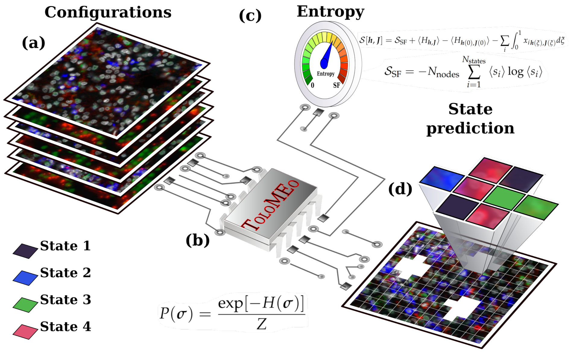
2. Method Overview
3. Materials and Methods
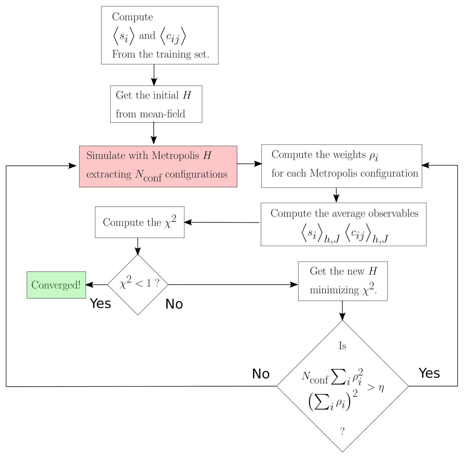
Dynamical Maximum Entropy
4. Results and Discussion
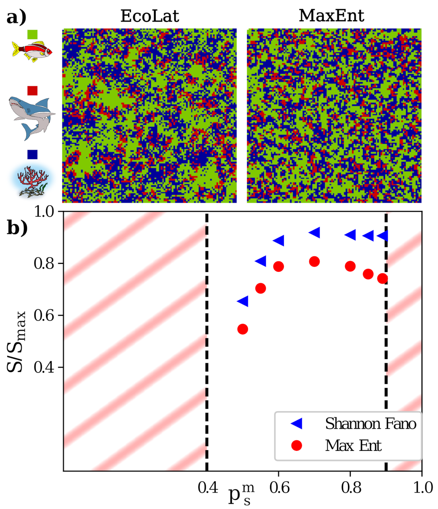
4.1. Agent Based Model on 2D Lattice: The EcoLat Model
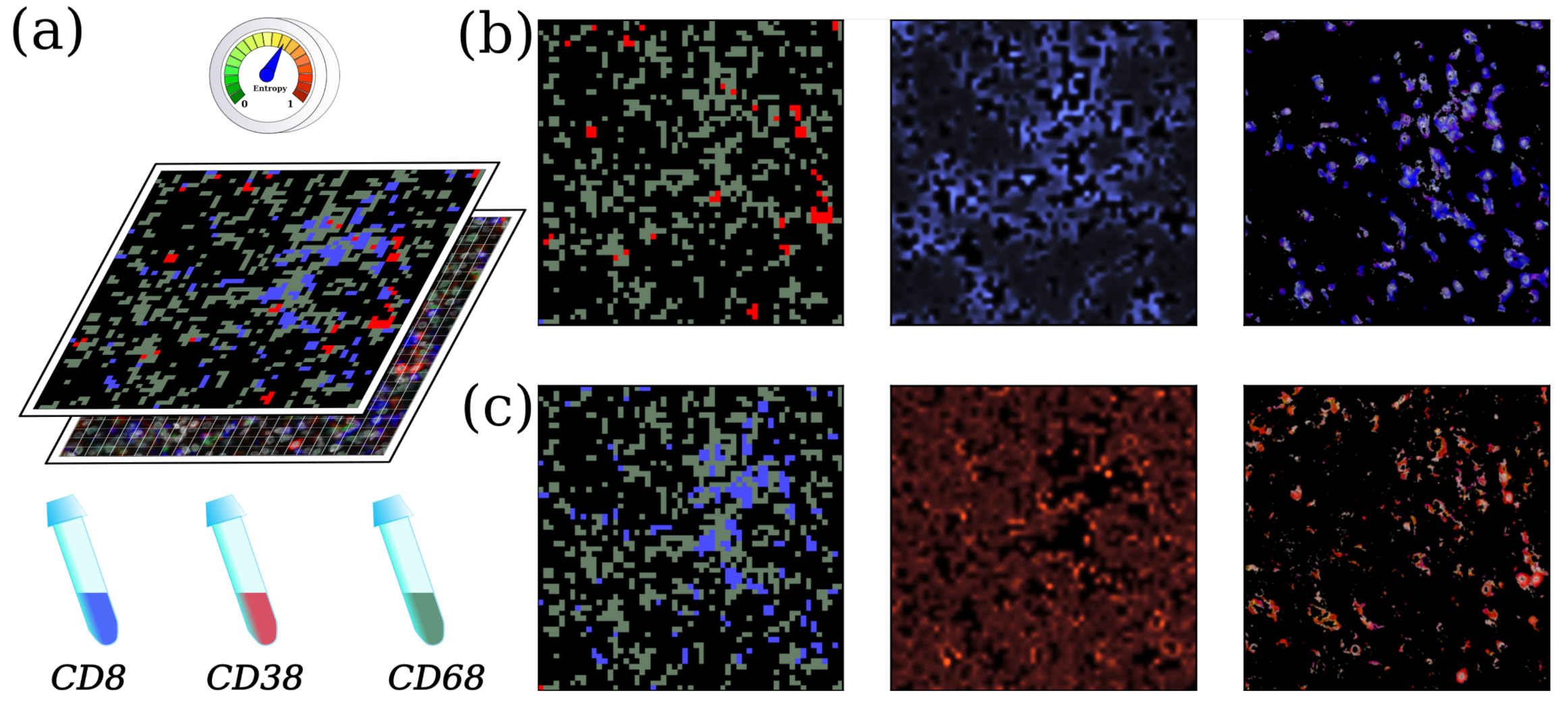
4.2. Biological Image Processing
4.3. General Network Models: The Hopfield Neural Network
5. Conclusions
Author Contributions
Funding
Data Availability Statement
Acknowledgments
Conflicts of Interest
Abbreviations
| SF | Shannon–Fano |
| MaxEnt | Maximum Entropy |
| ToloMEo | TOpoLogical netwOrk Maximum Entropy Optimiziation |
| NESS | Non-Equilibrium Steady-State |
| RNN | Recurrent Neural Networks |
References
- Bialek, W. Biophysics: Searching for Principles; Princeton University Press: Princeton, NJ, USA, 2012. [Google Scholar]
- Kleeman, R. Information Theory and Dynamical System Predictability. Entropy 2011, 13, 612–649. [Google Scholar] [CrossRef] [Green Version]
- De Martino, A.; De Martino, D. An introduction to the maximum entropy approach and its application to inference problems in biology. Heliyon 2018, 4, e00596. [Google Scholar] [CrossRef] [Green Version]
- Jakimowicz, A. The Role of Entropy in the Development of Economics. Entropy 2020, 22, 452. [Google Scholar] [CrossRef] [PubMed]
- Pressé, S.; Ghosh, K.; Lee, J.; Dill, K.A. Principles of maximum entropy and maximum caliber in statistical physics. Rev. Mod. Phys. 2013, 85, 1115. [Google Scholar] [CrossRef] [Green Version]
- Kelly, J.L. A New Interpretation of Information Rate. Bell Syst. Tech. J. 1956, 35, 917–926. [Google Scholar] [CrossRef]
- Kussell, E. Phenotypic Diversity, Population Growth, and Information in Fluctuating Environments. Science 2005, 309, 2075–2078. [Google Scholar] [CrossRef] [Green Version]
- Bialek, W.; Nemenman, I.; Tishby, N. Predictability, Complexity, and Learning. Neural Comput. 2001, 13, 2409–2463. [Google Scholar] [CrossRef]
- Bialek, W.; Cavagna, A.; Giardina, I.; Mora, T.; Silvestri, E.; Viale, M.; Walczak, A.M. Statistical mechanics for natural flocks of birds. Proc. Natl. Acad. Sci. USA 2012, 109, 4786–4791. [Google Scholar] [CrossRef] [Green Version]
- Stein, R.R.; Marks, D.S.; Sander, C. Inferring Pairwise Interactions from Biological Data Using Maximum-Entropy Probability Models. PLoS Comput. Biol. 2015, 11, e1004182. [Google Scholar] [CrossRef] [Green Version]
- De Martino, D.; Capuani, F.; De Martino, A. Quantifying the entropic cost of cellular growth control. Phys. Rev. E 2017, 96, 010401. [Google Scholar] [CrossRef] [Green Version]
- Cocco, S.; Leibler, S.; Monasson, R. Neuronal couplings between retinal ganglion cells inferred by efficient inverse statistical physics methods. Proc. Natl. Acad. Sci. USA 2009, 106, 14058–14062. [Google Scholar] [CrossRef] [Green Version]
- Ohiorhenuan, I.E.; Mechler, F.; Purpura, K.P.; Schmid, A.M.; Hu, Q.; Victor, J.D. Sparse coding and high-order correlations in fine-scale cortical networks. Nature 2010, 466, 617–621. [Google Scholar] [CrossRef]
- Schneidman, E.; Berry, M.J.; Segev, R.; Bialek, W. Weak pairwise correlations imply strongly correlated network states in a neural population. Nature 2006, 440, 1007–1012. [Google Scholar] [CrossRef] [Green Version]
- Weigt, M.; White, R.A.; Szurmant, H.; Hoch, J.A.; Hwa, T. Identification of direct residue contacts in protein-protein interaction by message passing. Proc. Natl. Acad. Sci. USA 2008, 106, 67–72. [Google Scholar] [CrossRef] [Green Version]
- Graeber, T.G.; Heath, J.R.; Skaggs, B.J.; Phelps, M.E.; Remacle, F.; Levine, R.D. Maximal entropy inference of oncogenicity from phosphorylation signaling. Proc. Natl. Acad. Sci. USA 2010, 107, 6112–6117. [Google Scholar] [CrossRef] [PubMed] [Green Version]
- Morcos, F.; Pagnani, A.; Lunt, B.; Bertolino, A.; Marks, D.S.; Sander, C.; Zecchina, R.; Onuchic, J.N.; Hwa, T.; Weigt, M. Direct-coupling analysis of residue coevolution captures native contacts across many protein families. Proc. Natl. Acad. Sci. USA 2011, 108, E1293–E1301. [Google Scholar] [CrossRef] [Green Version]
- Santolini, M.; Mora, T.; Hakim, V. A General Pairwise Interaction Model Provides an Accurate Description of In Vivo Transcription Factor Binding Sites. PLoS ONE 2014, 9, e99015. [Google Scholar] [CrossRef] [Green Version]
- Mora, T.; Walczak, A.M.; Bialek, W.; Callan, C.G. Maximum entropy models for antibody diversity. Proc. Natl. Acad. Sci. USA 2010, 107, 5405–5410. [Google Scholar] [CrossRef] [Green Version]
- Cavagna, A.; Giardina, I.; Ginelli, F.; Mora, T.; Piovani, D.; Tavarone, R.; Walczak, A.M. Dynamical maximum entropy approach to flocking. Phys. Rev. E 2014, 89, 042707. [Google Scholar] [CrossRef] [Green Version]
- Miotto, M.; Monacelli, L. Entropy evaluation sheds light on ecosystem complexity. Phys. Rev. E 2018, 98, 042402. [Google Scholar] [CrossRef] [Green Version]
- Volkov, I.; Banavar, J.R.; Hubbell, S.P.; Maritan, A. Inferring species interactions in tropical forests. Proc. Natl. Acad. Sci. USA 2009, 106, 13854–13859. [Google Scholar] [CrossRef] [PubMed] [Green Version]
- Folli, V.; Gosti, G.; Leonetti, M.; Ruocco, G. Effect of dilution in asymmetric recurrent neural networks. Neural Netw. 2018, 104, 50–59. [Google Scholar] [CrossRef] [PubMed]
- Gosti, G.; Folli, V.; Leonetti, M.; Ruocco, G. Beyond the Maximum Storage Capacity Limit in Hopfield Recurrent Neural Networks. Entropy 2019, 21, 726. [Google Scholar] [CrossRef] [Green Version]
- Shore, J.; Johnson, R. Axiomatic derivation of the principle of maximum entropy and the principle of minimum cross-entropy. IEEE Trans. Inf. Theory 1980, 26, 26–37. [Google Scholar] [CrossRef] [Green Version]
- Miotto, M.; Monacelli, L. Genome heterogeneity drives the evolution of species. Phys. Rev. Res. 2020, 2, 043026. [Google Scholar] [CrossRef]
- Monacelli, L.; Errea, I.; Calandra, M.; Mauri, F. Pressure and stress tensor of complex anharmonic crystals within the stochastic self-consistent harmonic approximation. Phys. Rev. B 2018, 98. [Google Scholar] [CrossRef] [Green Version]
- Monacelli, L.; Bianco, R.; Cherubini, M.; Calandra, M.; Errea, I.; Mauri, F. The Stochastic Self-Consistent Harmonic Approximation: Calculating Vibrational Properties of Materials with Full Quantum and Anharmonic Effects. J. Phys. Condens. Matter 2021. [Google Scholar] [CrossRef]
- Castellana, M.; Bialek, W.; Cavagna, A.; Giardina, I. Entropic effects in a nonequilibrium system: Flocks of birds. Phys. Rev. E 2016, 93, 052416. [Google Scholar] [CrossRef] [Green Version]
- Chopard, B.; Dupuis, A.; Masselot, A.; Luthi, P. Cellular automata and lattice Boltzmann techniques: An approach to model and simulate complex systems. Adv. Complex Syst. 2002, 05, 103–246. [Google Scholar] [CrossRef]
- Chevrier, S.; Levine, J.H.; Zanotelli, V.R.T.; Silina, K.; Schulz, D.; Bacac, M.; Ries, C.H.; Ailles, L.; Jewett, M.A.S.; Moch, H.; et al. An Immune Atlas of Clear Cell Renal Cell Carcinoma. Cell 2017, 169, 736–749.e18. [Google Scholar] [CrossRef] [Green Version]
- Schulz, D.; Zanotelli, V.R.T.; Fischer, J.R.; Schapiro, D.; Engler, S.; Lun, X.K.; Jackson, H.W.; Bodenmiller, B. Simultaneous Multiplexed Imaging of mRNA and Proteins with Subcellular Resolution in Breast Cancer Tissue Samples by Mass Cytometry. Cell Syst. 2018, 6, 25–36.e5. [Google Scholar] [CrossRef] [Green Version]
- Chiang, C.W.; Chuang, E.Y. Biofunctional core-shell polypyrrole and polyethylenimine nanocomplex for a locally sustained photothermal with reactive oxygen species enhanced therapeutic effect against lung cancer. Int. J. Nanomed. 2019, 14, 1575–1585. [Google Scholar] [CrossRef] [PubMed] [Green Version]
- Enrico Bena, C.; Del Giudice, M.; Grob, A.; Gueudré, T.; Miotto, M.; Gialama, D.; Osella, M.; Turco, E.; Ceroni, F.; De Martino, A.; et al. Initial cell density encodes proliferative potential in cancer cell populations. Sci. Rep. 2021, 11, 6101. [Google Scholar] [CrossRef]
- Grecco, H.E.; Imtiaz, S.; Zamir, E. Multiplexed imaging of intracellular protein networks. Cytometry Part A 2016, 89, 761–775. [Google Scholar] [CrossRef]
- Peruzzi, G.; Miotto, M.; Maggio, R.; Ruocco, G.; Gosti, G. Asymmetric binomial statistics explains organelle partitioning variance in cancer cell proliferation. Commun. Phys. 2021, 4. [Google Scholar] [CrossRef]
- Klauschen, F.; Ishii, M.; Qi, H.; Bajénoff, M.; Egen, J.G.; Germain, R.N.; Meier-Schellersheim, M. Quantifying cellular interaction dynamics in 3D fluorescence microscopy data. Nat. Protoc. 2009, 4, 1305–1311. [Google Scholar] [CrossRef] [PubMed] [Green Version]
- Hopfield, J.J. Neural networks and physical systems with emergent collective computational abilities. Proc. Natl. Acad. Sci. USA 1982, 79, 2554–2558. [Google Scholar] [CrossRef] [Green Version]
- Marullo, C.; Agliari, E. Boltzmann Machines as Generalized Hopfield Networks: A Review of Recent Results and Outlooks. Entropy 2020, 23, 34. [Google Scholar] [CrossRef]
- Bastolla, U.; Parisi, G. Relaxation, closing probabilities and transition from oscillatory to chaotic attractors in asymmetric neural networks. J. Phys. Math. Gen. 1998, 31, 4583. [Google Scholar] [CrossRef] [Green Version]
- Gutfreund, H.; Reger, J.; Young, A. The nature of attractors in an asymmetric spin glass with deterministic dynamics. J. Phys. Math. Gen. 1988, 21, 2775. [Google Scholar] [CrossRef]
- Tang, G.; Gudsnuk, K.; Kuo, S.H.; Cotrina, M.L.; Rosoklija, G.; Sosunov, A.; Sonders, M.S.; Kanter, E.; Castagna, C.; Yamamoto, A.; et al. Loss of mTOR-dependent macroautophagy causes autistic-like synaptic pruning deficits. Neuron 2014, 83, 1131–1143. [Google Scholar] [CrossRef] [Green Version]
- Perin, R.; Berger, T.K.; Markram, H. A synaptic organizing principle for cortical neuronal groups. Proc. Natl. Acad. Sci. USA 2011, 108, 5419–5424. [Google Scholar] [CrossRef] [Green Version]
- Witter, M.P. Connectivity of the Hippocampus; Springer: New York, NY, USA, 2010; pp. 5–26. [Google Scholar]
- Leonetti, M.; Folli, V.; Milanetti, E.; Ruocco, G.; Gosti, G. Network dilution and asymmetry in an efficient brain. Philos. Mag. 2020, 100, 2544–2555. [Google Scholar] [CrossRef] [Green Version]


Publisher’s Note: MDPI stays neutral with regard to jurisdictional claims in published maps and institutional affiliations. |
© 2021 by the authors. Licensee MDPI, Basel, Switzerland. This article is an open access article distributed under the terms and conditions of the Creative Commons Attribution (CC BY) license (https://creativecommons.org/licenses/by/4.0/).
Share and Cite
Miotto, M.; Monacelli, L. TOLOMEO, a Novel Machine Learning Algorithm to Measure Information and Order in Correlated Networks and Predict Their State. Entropy 2021, 23, 1138. https://doi.org/10.3390/e23091138
Miotto M, Monacelli L. TOLOMEO, a Novel Machine Learning Algorithm to Measure Information and Order in Correlated Networks and Predict Their State. Entropy. 2021; 23(9):1138. https://doi.org/10.3390/e23091138
Chicago/Turabian StyleMiotto, Mattia, and Lorenzo Monacelli. 2021. "TOLOMEO, a Novel Machine Learning Algorithm to Measure Information and Order in Correlated Networks and Predict Their State" Entropy 23, no. 9: 1138. https://doi.org/10.3390/e23091138
APA StyleMiotto, M., & Monacelli, L. (2021). TOLOMEO, a Novel Machine Learning Algorithm to Measure Information and Order in Correlated Networks and Predict Their State. Entropy, 23(9), 1138. https://doi.org/10.3390/e23091138