1. Introduction
In a nonlinear dynamical system, the average rate of divergence of the trajectories in the state space is captured by the largest Lyapunov exponent [
1]. This is also the rate at which the dynamical system
loses information related to the initial condition or, equivalently, the rate at which information is
generated [
2]. Motivated by the objective of distinguishing chaotic systems from periodic and stochastic systems, early works of Grassberger and Procaccia [
3], Takens [
4], and Eckmann and Ruelle [
5] proposed practical means of estimating the Kolmogorov–Sinai entropy, using a time series.
Inspired by many inconclusive results arising from practical applications of the Kolmogorov–Sinai entropy [
6,
7], Pincus [
8] recognized that, even when only a limited amount of data is available and the system lacks stationary behavior, entropy can still be effectively employed to measure the
complexity or the degree of
repeatability of a time series and, indirectly, of the system that generated this series. Since then, the use of statistics quantifying the entropy rate of a time series has flourished, especially for biological series. However, real signals are inherently contaminated by noise. To deal with an arbitrary series of observations, Bandt and Pompe [
9] suggested avoiding the problem altogether by measuring the entropy of the probability distribution of ordinal patterns, which, in the limit, provides an upper bound for the Kolmogorov–Sinai entropy [
10].
Along this line, bubble entropy [
11] was introduced to quantify the complexity of a time series by measuring the entropy of the series of swaps necessary to (bubble) sort its portions. Thus,
complexity is intended not as a lack of similar patterns but as added diversity in the ordering of the samples across scales. As such, bubble entropy (
) does not directly quantify the entropy rate of the series, as Approximate Entropy (
) [
8] and Sample Entropy (
) [
12] do, nor the entropy of the distribution of the possible permutations, as Permutation Entropy (
) does.
measures the increase in the entropy of the series of sorting steps (swaps), necessary to order its portions of length
m, when adding an extra element.
On the bright side, is an entropy metric, with a limited dependence on parameters. This is a clear advantage over the other estimators, for which the selection of the values of the parameters is critical. The computed values, as well as the discriminating power of the estimators, depend on the parameters, and careful estimation is essential. Taking into account that this estimation can be proven to be application- or data-dependent, the minimal dependence on parameters becomes an even more important property.
Both and need to estimate two parameters: the threshold distance r and the embedding dimension m. In practice, we have accepted that the best we can do currently is to omit this step and recruit the typical values: or 2, when the length of the series permits it, and . In a more advantageous position, , similarly to , requires the estimation of only one parameter: the embedding dimension m. Not only are the degrees of freedom reduced to 1 but the remaining parameter is also an integer number, whilst the eliminated one is real.
The embedding dimension
m ranges from 1 to a small integer value, allowing a systematic estimation of all reasonable values. On the other hand, the domain of
r is an infinite set, making the consideration of all possible, or even reasonable, values impossible. For a detailed comparison of bubble entropy with other popular entropy metrics, please refer to [
11]. In general, when tested on real data (e.g., the same datasets that are going to be considered in this paper),
displayed higher discriminating power over
,
, and
, for most values of
m.
An analytical formulation of
for the autoregressive (AR) processes was recently made available [
13]. This showed that, at least for this class of processes, the relation between the first autocorrelation coefficient and
changes for odd and even values of
m. The authors also pointed out that the largest value of
did not arise for white noise but when correlations were large. While these are not issues per se, they triggered the idea that further refinements and understanding of the definition might be possible.
In this paper, we improve the comprehension of the metric, using theoretical considerations on the expected values for AR processes. We investigate a two-steps-ahead estimator of
, which considers the cost of ordering two additional samples. We also consider a new normalization factor that gives entropy values
for white Gaussian noise (WGN). The rest of the paper is structured as follows.
Section 3 investigates the examined normalization factor.
Section 4 presents theoretical issues and simulations on the examined two-steps-ahead estimator, and
Section 5 uses real HRV signals to evaluate the estimator in a real world problem. There is some discussion in
Section 6, whilst the last section concludes this work.
2. Bubble Entropy as a Measure of Complexity
embeds a given time series
of size
N into an
m dimensional space, producing a series of vectors of size
:
Each vector
is sorted using the
bubble sort algorithm, and the number of swaps (inversions) required for sorting is counted.
The probability mass function (
pmf)
of having
i swaps is used to evaluate the second-order Rényi Entropy:
while the
is estimated as the normalized difference of the entropy of the swaps required for sorting vectors of length
and
m:
Vectors
are sorted in ascending order; this is only a convention, which does not affect the time series categorization, nor the value of
. Indeed, if we refer to
as to the number of swaps required to sort the vector
in ascending order, then to sort it in descending order,
sorting steps are necessary. As such, if
is the
pmf of the swaps required for sorting all the vectors in ascending order, then sorting them in descending order will produce the
pmf , which leads to an identical value of
in Equation (
2).
In order to make the definition even more comprehensive, we give below an algorithmic description of the computation of :
step 1: Compute entropy in m dimensional space:
step 1.1: embed the signal into m dimensional space
step 1.2: for each vector, compute the number of swaps required by the bubble sort to sort it
step 1.3: construct a series with the computed number of swaps
step 1.4: use Rényi entropy (order 2) to compute entropy on this series
step 2: Compute entropy in m+1 dimensional space
step 3: Report the difference of entropy computed in steps 1 and 2
From the standard results in information theory [
14], it is possible to cast further light on
. The entropy of the sum of two variables
is always smaller or equal to their joint entropy
. Hence:
. The number of swaps
required to sort a vector of length
is a random variable, obtained by adding a random number of steps
, needed to sort a vector of length
m, plus the extra swaps
to take the new sample in its ordered position:
Setting
and
in the relation just derived, and remembering that the mutual information:
, then:
or:
is, therefore, limited from above by the entropy of the number of swaps required to add the extra element in the vector, reduced by the information already carried by the number of swaps performed before.
In the following, we will use the term , instead of simply , which has been used until now. We want to make a clear distinction between this definition and an alternative one, which will be considered later in this paper.
3. On the Investigation of the Normalization Factor
The normalization factor
in Equation (
3) is given by the difference in the maximum swaps quadratic entropy, which is
for the embedding dimension
m and
for embedding dimension
, when neglecting the term
in the logarithms. This term corresponds to the
no swaps performed state and the simplification contributes toward a more elegant definition, without significant influence on the numerical value, especially for larger values of
m.
Common definitions of entropy present maximum entropy values when WGN is given as the input. However, in our previous work [
13], we showed that
is not maximal for WGN. Signals produced by the AR model with large and positive one-step autocorrelation tended to require a broader range of swaps than WGN, and the uniform distribution had the largest entropy among all discrete probability mass functions. We will come back to this observation, after we introduce one more definition:
.
The analytical value of
for WGN can be obtained in a simpler fashion than that described in [
13]. The probability generating function of the number of inversions required to sort a random permutation of
m numbers [
15] is given by:
Indeed, according to Equation (
5), the total number of swaps required for a WGN is a random variable obtained as the sum of
m independent discrete uniform random variables with support
and
. Thus, given
k samples, which are already sorted, a new random value in position
requires any from 0 to
k inversions, each with the probability
, to be swapped into the correct position. The probability generating function for the number of additional inversions is:
. The probability generating function of the total number of inversions
is given as the product of the additional permutations and
, where
:
As the number of permutations with no inversions is 1, we can obtain Equation (
8).
Then, from the definition of the probability generating function, the
pmf , having
i swaps, is the coefficient of the
i-order term in the polynomial
, or:
The entropy of the series of swaps, for WGN, is a growing function with
m:
and the
of a WGN:
Having now the values of entropy of the series of swaps for a WGN, for any value of
m, we define, as
, the ratio:
In other words,
is the difference of the entropy in the dimensional spaces
and
m, normalized with the difference of the entropy of WGN in these spaces.
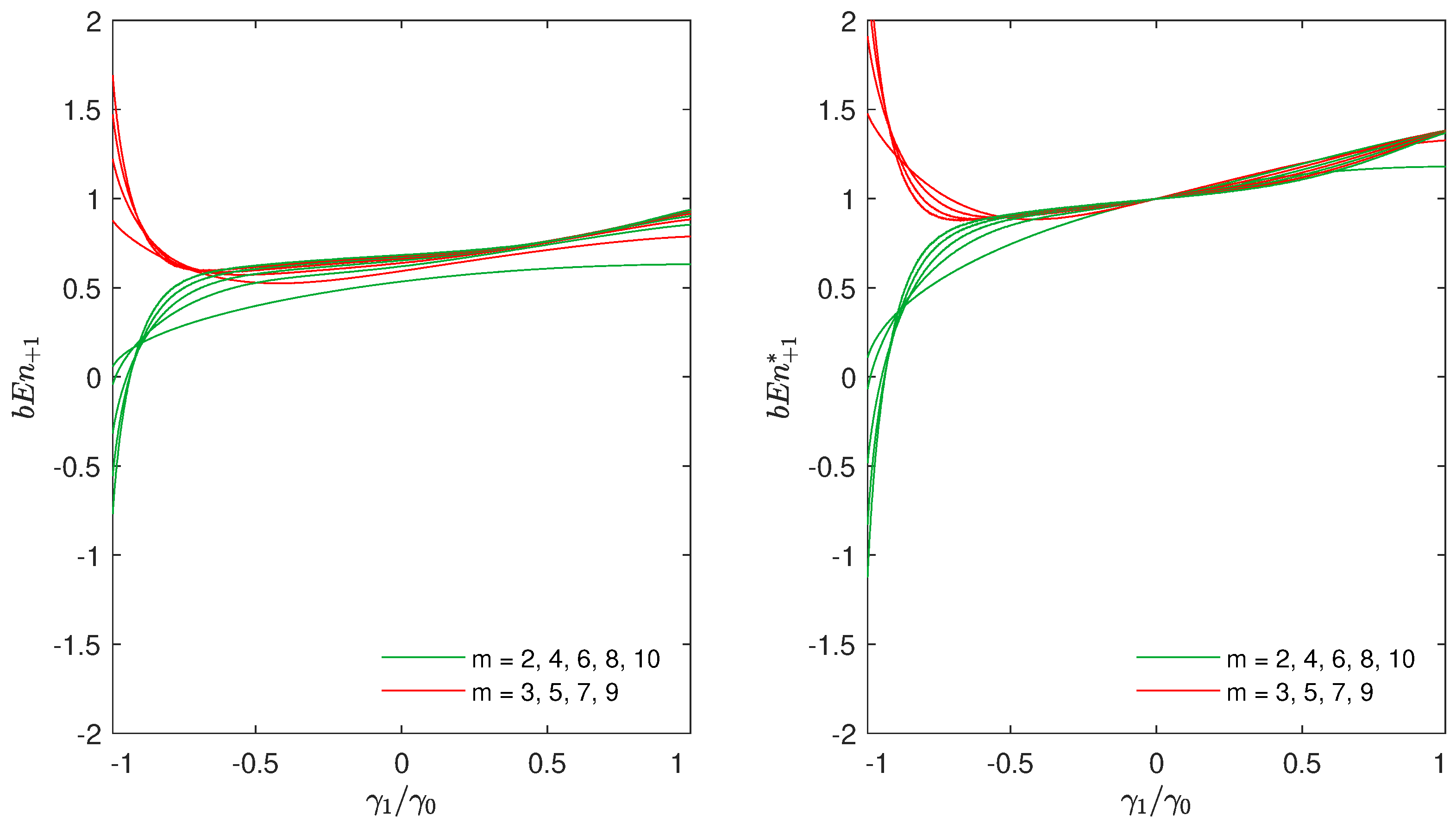
Let us cover the benefits of using this definition. In
Figure 1, we generate a series from the AR process of order 1:
where
, and
is WGN with the mean
and variance
. The correlation at lag
k is
and
. Numerical estimates of
were computed over 1000 Monte Carlo simulations with a series of
samples.
In the subfigure on the left hand side of
Figure 1, we used the definition of
, as we did in [
13]. In the subfigure on the right hand side of the figure, we can see the difference, in the same experiment, when
was used. Please note that, with the definition of
, the entropy for WGN (
) is equal to 1 for all values of
m.
Since, this is an important property, we found the normalization proposed in Equation (
13) to be more appropriate than the one in Equation (
3), which was used until now. In fact, values of bubble entropy computed with this normalization can be used to compare different processes and/or to put them in relation with WGN (a
larger than one means that the
pmf of the number of swaps becomes more “spread out” than for a WGN, when
m increases). This normalization further reduces the dependence on the residual parameter
m, as nearly identical values of
for
and
in the right panel of
Figure 1 show.
The value of
in Equation (
11) is exact; however, its computation is challenging for large values of
m, due to the growth of the factorial term. However, in this situation, when
m is large, for the central limit theorem, the discrete
pmf converges in distribution to a normal probability density function (
pdf), with the same mean and variance. Due to the symmetry of the
pmf, the mean of
is
, which can also be obtained as
. The variance can be obtained from the probability generating function:
Alternatively,
can be computed by observing that the variance of the discrete uniform distribution has the probability generating function
is
. The total number of inversions is the sum of
m independent random variables and, as a consequence,
is the sum of the single variances:
The Rényi entropy of order 2 (or quadratic entropy) of a normal
pdf is
, where
is its variance. When
m is large, we can then approximate the entropy of the series of swaps for a WGN with:
In our numerical tests, the approximation holds well for values of
, where the error is already smaller than 1
. For smaller values of
m, Equation (
11) should be employed instead.
4. On the Investigation of the Two-Step-Ahead Estimator of Bubble Entropy
Let us stay for a while at
Figure 1. In both subfigures of
Figure 1, for anti-persistent noise, i.e., when
approaches
, the values of entropy become negative for even values of
m, whilst they are largely positive for odd values of
m. This is another issue that gives us motivation for further investigation.
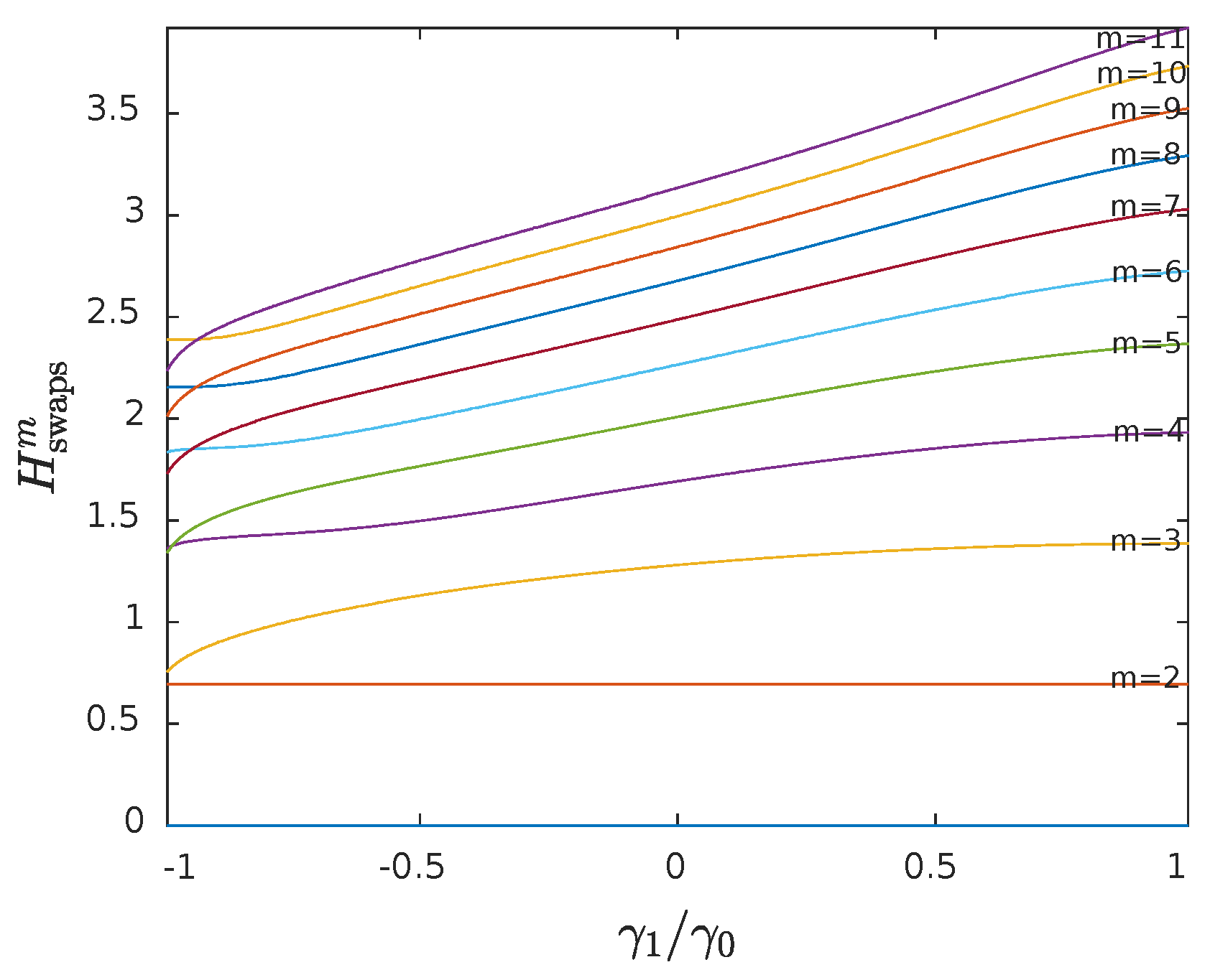
In
Figure 2, the average numerical values of
for
are presented, using the same simulations described in
Figure 1. The lines at the lower part of the figure correspond to lower values of
m. When
m is even and
is approaching to
, we can observe that
is a possible condition, something that results in negative values (
).
Even though this is not a problem per se, to further analyze this observation, we plotted the
pmfs in
Figure 3. In this figure, four
pmfs obtained from the 1st order AR model, averaging over 100 Monte Carlo runs, with the series length
, are displayed. The four
pmfs express the number of swaps necessary to sort: (a) an
long sequence with
, that is WGN; (b) an
long sequence with
, that is a random walk; (c) an
long sequence with
, that is an anti-persistent noise; and (d) an
long sequence with
depicting again anti-persistent noise.
It is interesting to note that, given the fact that WGN does not display the largest value of , its pmf is more concentrated around the average than that of the random walk. More interesting is the observation that the pmf of the anti-persistent noise is further concentrated around the mean. In the case in which , two peaks appear at .
This is something that occurs generally for even values of m. In fact, sorting the degenerate limit sequence always requires swaps more than sorting the series . On the contrary, for odd values of m, there is always only a single peak at , since sorting the series and has the same cost: . To illustrate this single peak, the pmf for and is also included in the figure. The larger spread around the mean, due to the two peaks appearing for even values of m, explains why is possible.
The above conclusions led us to define a two-steps-ahead estimator for bubble entropy by setting:
In other words, instead of computing the difference in entropy between spaces with dimensions
m and
, we consider the variation between the spaces
m and
(hence the pedix
instead of
). This consideration allows us to compare the number of swaps required to sort the vectors belonging to odd dimensional spaces (
m odd) with odd dimensional spaces (
odd) and even dimensional spaces (
m even) with even dimensional spaces (
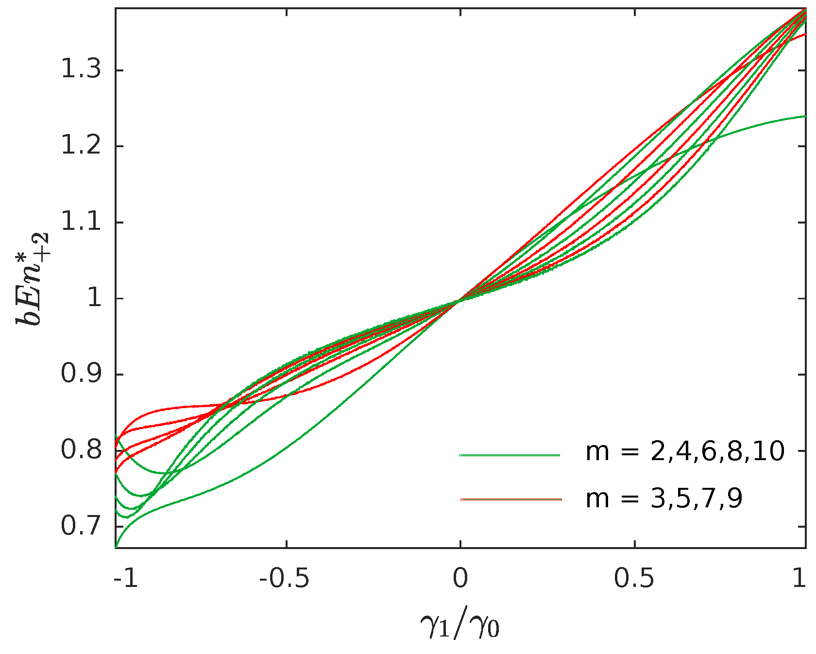
even), eliminating the asymmetry detected between odd and even spaces. It also leads to positive and growing entropy values, as shown in
Figure 4, in contrast to the behavior observed in
Figure 1.
To rationalize the relation between
and
, we notice that:
Indeed:
and, in practical applications, where empirically
is found to decrease with
m:
When
m is large, the two bracketing values approach and:
or, equivalently, for a WGN:
While Equation (
23) is exact for a stationary process in the limit
, we empirically verified that it holds sufficiently well for “practical” values of
m. For example, the difference is smaller than
when
.
Now, taking the ratio side by side of Equations (
22) and (
23), we derive that:
Therefore, the two estimators provide estimates that are quantitatively equivalent (e.g., both are 1 for a WGN).
5. Experimental Analysis
In order to support our theoretical considerations, we tested our observations on real HRV signals as well, obtained from Physionet [
16]. The first data set is the
Normal Sinus Rhythm (NSR) RR Interval Database (
nsr2db). This database includes beat annotations for 54 long-term ECG recordings of subjects in normal sinus rhythm (30 men, aged 28.5 to 76, and 24 women, aged 58 to 73). The original ECG recordings were digitized at 128 samples per second, and the beat annotations were obtained by automated analysis with manual review and correction.
The second data set is the Congestive Heart Failure (CHF) RR Interval Database (chf2db). This database includes beat annotations for 29 long-term ECG recordings of subjects aged 34 to 79 years, with congestive heart failure (NYHA classes I, II, and III). The subjects included eight men and two women; gender was not known for the remaining 21 subjects. The original ECG recordings were digitized at 128 samples per second, and the beat annotations were also obtained by automated analysis with manual review and correction.
The HRV series were obtained from the beat annotation files. Only normal-to-normal beat intervals were considered. To reduce the impact of artifacts on the estimates of the metrics, we removed all NN intervals, which differed more than 30% from the previous NN interval.
Our target was to compare the discriminating power of the two definitions of bubble entropy,
and
, to separate the two groups of subjects. We used
p-values (the Mann–Whitney U test) as a criterion. We computed the bubble entropy for
and
for values of
m ranging from
to
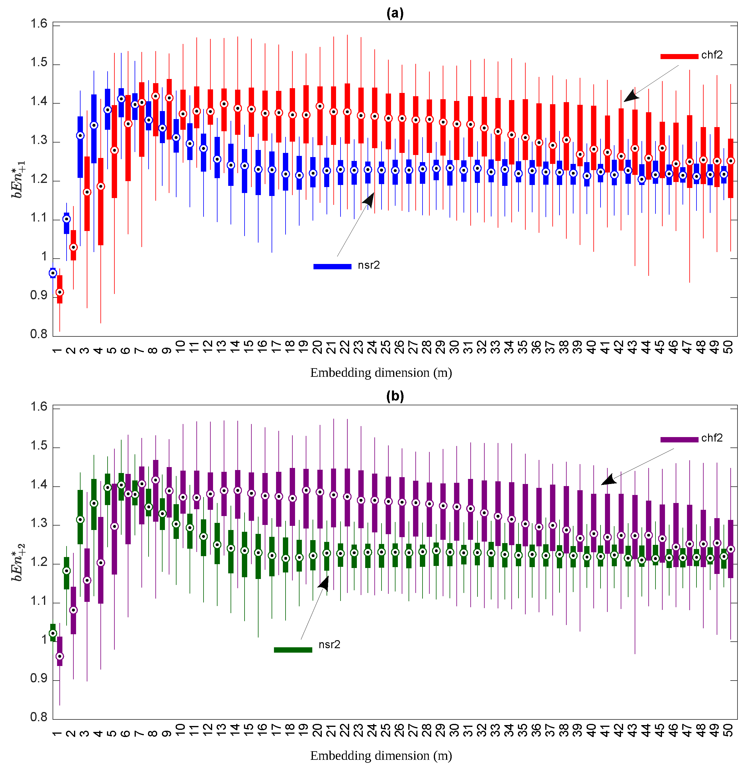
. In
Figure 5, we present the box plots for both
(the top subfigure of
Figure 5) and
(the bottom subfigure or
Figure 5).
For the simulations and as expected from the theoretical considerations, the values of
and
were similar. Normal subjects displayed a
that was larger than CHF patients for small values of
m (≤5), while it became smaller when
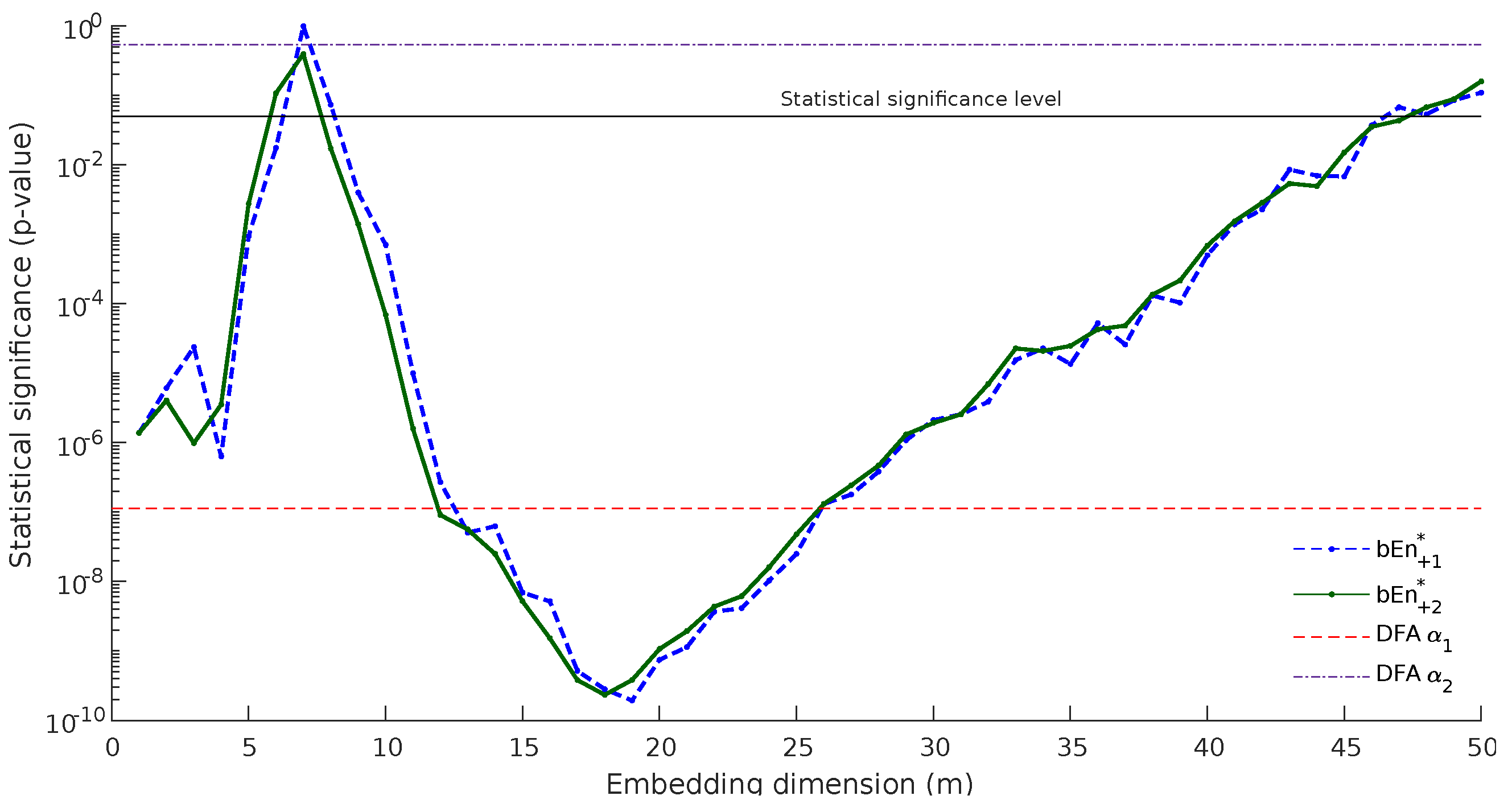
m is large. The results of the statistical test are depicted in
Figure 6. The blue dashed line represents
p-values computed with
, whilst the green line shows the corresponding
p-values for
. Please note that this is a log plot. There are two main conclusions from this graph:
The p-values computed by were smaller than those computed with , especially in the region of , where the method appeared to succeed with better classification, which improved as m increased.
presented a smoother behavior, especially in the same area: . This is in accordance with the our main hypothesis that the method behaves in a different way for odd and even values of m.
In order to have a better sense of the discriminating power of the method, we marked on
Figure 6 the statistical significance level (blue solid line at 0.05) and the
p-values computed by Detrended Fluctuation Analysis (DFA) [
17], index DFA
, and DFA
. In the context of HRV series obtained from 24-h Holter recordings, the slope DFA
is typically found to be in the range
for normal subjects, DFA
for CHF patients and DFA
for subjects who survived a myocardial infarction [
18]. Bubble entropy always presents significantly better categorization than DFA
and better categorization than DFA
for
.
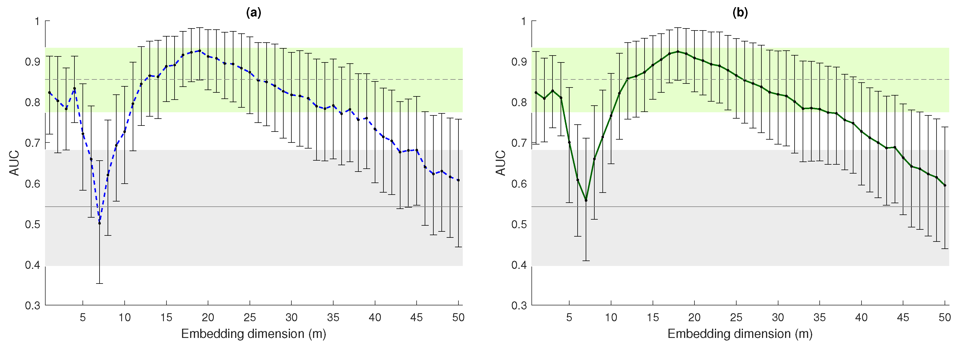
For completeness, in
Figure 7, we present the Area-Under-the-ROC-Curve (AUC) computed when using either
and
to discrimnate the two populations. We also included the 95% confidence intervals, computed using bootstrap (1000 iterations), to compensate for the low dimension of the two populations. Coherent conclusions can be drawn from these plots. The results in the figure confirm that
discriminated the HRV series of normal subjects and CHF patients when
m was small (
) with an AUC comparable to DFA
. We speculate that the characteristics of the signal they are picking up might be the same.
Then, shows a very large AUC also for about . While DFA detects the long-term memory characteristics of the series, it does not distinguish between the two populations, so the features detected by might be different. Of note, the definition of permits the exploration of ranges of m, which are not typically accessible with other entropy measures, such as ApEn or SampEn (m was rarely larger then 3, due to convergence issues) or Permutation Entropy (typical values of m are smaller than 10 as the factorial terms increase very quickly).
6. Discussion
Even though this paper examines alternatives in the definition of bubble entropy, we took the opportunity to summarize in this last section some conclusions on the comparison of bubble entropy with other popular definitions, especially in the m-dimensional space.
Definitions in the m-dimensional space extract more sensitive information compared with the more classic definitions in 1-dimensional space. They not only exploited the values of the samples but also their order. If, for example, we shuffle the samples of a time series, the values of both Shannon and Rényi entropy will be unaffected. Due to their increased sensitivity, definitions in m-dimensional space became quite popular and are valuable tools in entropy analysis.
Approximate and sample entropy are almost always used in research work involving entropy analysis, especially in biological signals. We chose to compare bubble entropy with those widely accepted estimators. We already discussed, in the introductory section, the main advantages of bubble entropy analysis against approximate and sample entropy, emphasizing the minimal dependence on parameters. We also discussed the discriminating power, not only for approximate and sample entropy but also for permutation entropy, an entropy metric that inspired bubble entropy.
As stated above, it was not the objective of this paper to make a comparison between bubble entropy and other entropy metrics. For this, we refer the interested reader to our previous work [
11]. However, to add perspective, we included into
Figure 6 and
Figure 7 the values of DFA
and
. Detrended fluctuation analysis does not quantify entropy-related metrics, but it is a “fractal” method that proved effective in distinguishing healthy subjects from CHF patients [
18]. The values of DFA
are also related to the Hurst exponent for long-term memory processes, as well as bubble entropy in [
19].
7. Conclusions
The contributions of this paper are two-fold. First, we introduced an alternative normalization factor for bubble entropy, based on the theoretical value of bubble entropy, when WGN is given as input. With the new normalization factor, the entropy of WGN is always equal to 1, for every value of m. While theoretically interesting, this consideration does not affect the discriminating power of the method, since this is only a common scalar value.
The second contribution of this paper is the investigation of a two-steps-ahead estimator for bubble entropy. Since we showed that (rarely) is there (when the series are strongly anti-correlated) an asymmetry in the cost of bubble sorting between odd and even dimensional spaces, we computed the bubble entropy to compare the entropy between embedding spaces with odd dimensions or between embedding spaces with even dimensions. The advantage of this approach was illustrated with experiments with both simulated and real HRV signals.
The simulated WGN signals showed that, for anti-persistent noise, where the asymmetry between spaces with odd and even dimensions was maximally expressed, bubble entropy presented similar values for all values of m, in contrast to the initial approach, where the entropy values for anti-persistent noise were significantly different between successive values of m. Theoretically, this consideration improves the discriminating power of the method, even though conditions similar to strongly anti-persistent noise are not often found in HRV signals.
For completeness, we performed experiments with real HRV signals, which were publicly available and are widely used. The experiments showed that both examined definitions showed comparable discriminating power between the NSR and CHF signals. However, for values of , the two-steps-ahead estimator presented slightly higher statistical significance and more regular behavior, with a smoother difference between successive values of m.
The research increased our understanding of bubble entropy, in particular in the context of HRV analysis. The two-steps-ahead estimator, while a minor refinement, should not be ignored in future research directions.


