
Adaptive Diagnosis for Fault Tolerant Data Fusion Based on α-Rényi Divergence Strategy for Vehicle Localization


Abstract
1. Introduction
- Localization: being the ability to know how to define more or less precisely, and in an absolute or relative way, its position;
- Perception: knowing how to analyze the nearby environment and act accordingly (detection of obstacles, signaling, etc.);
- Control: take control of the vehicle’s actuators (acceleration, braking, steering angle, etc.); and,
- Navigation: knowing how to plan and execute a route to a destination.
2. Problem Statement
2.1. Diagnostic as a Guarantee of Safety
2.2. Fault Tolerance as an Availability Booster
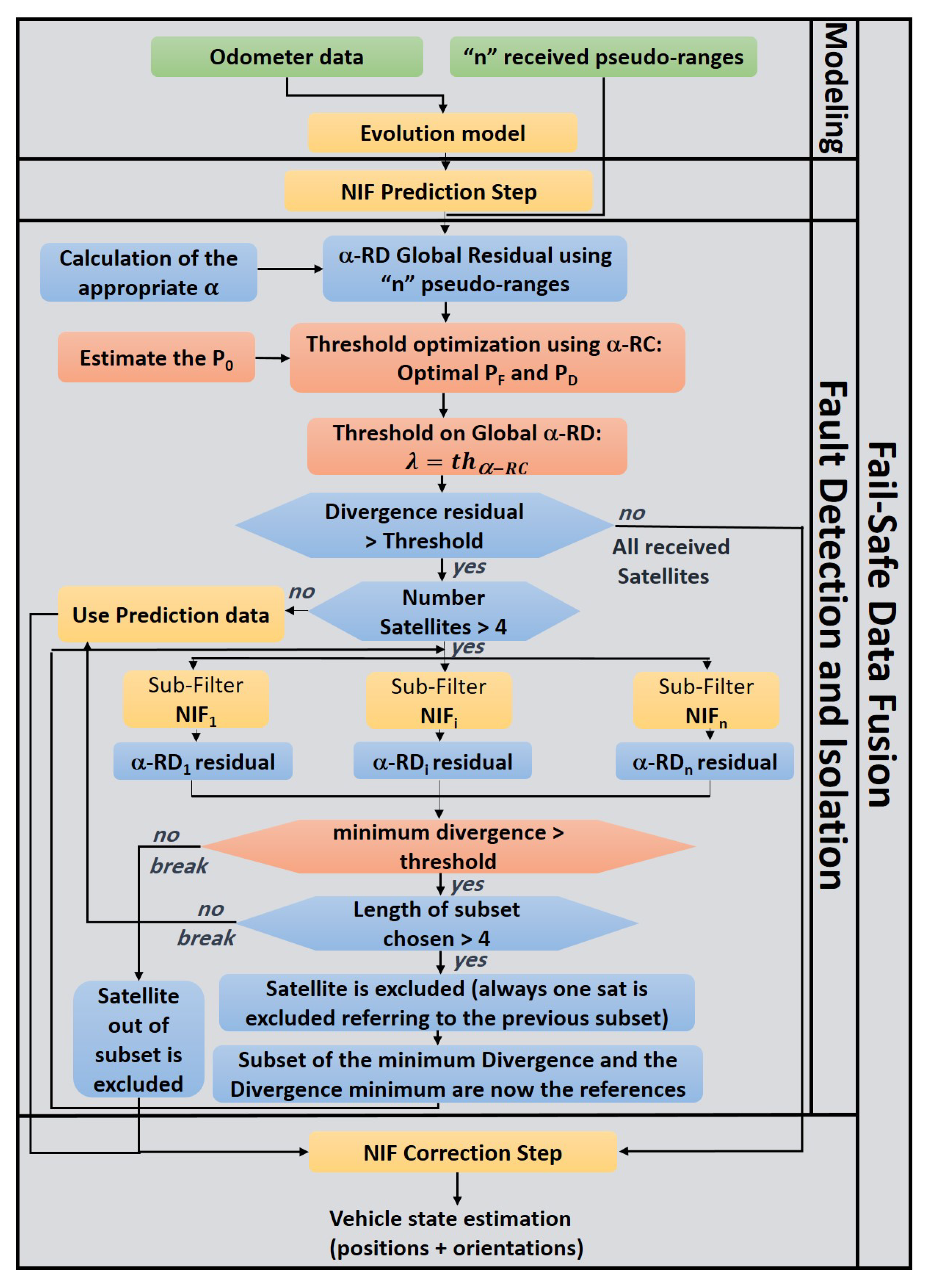
2.3. Proposed Approach Block Diagram
3. Nonlinear Information Filter
4. Adaptive Diagnostic Layer Based on -Rényi Divergence
4.1. -Rényi Divergence as a Parametric Residual
- The first test:represented by the weighted Mahalanobis distance, is to measure the distance between the means, while taking the value into consideration, which weights distance through its impact on the covariance matrices,
- The second test: , can be compared to the weighted Bregman, while taking the weight of for each covariance matrice into account,
- The third test: , represented by the weighted MI, where, in this test, the two pdfs are compared based on their weighting value related to the value of .
4.2. Establish a Residuals Parameterization Policy Based on Operational Requirements and Changes in Navigation Context
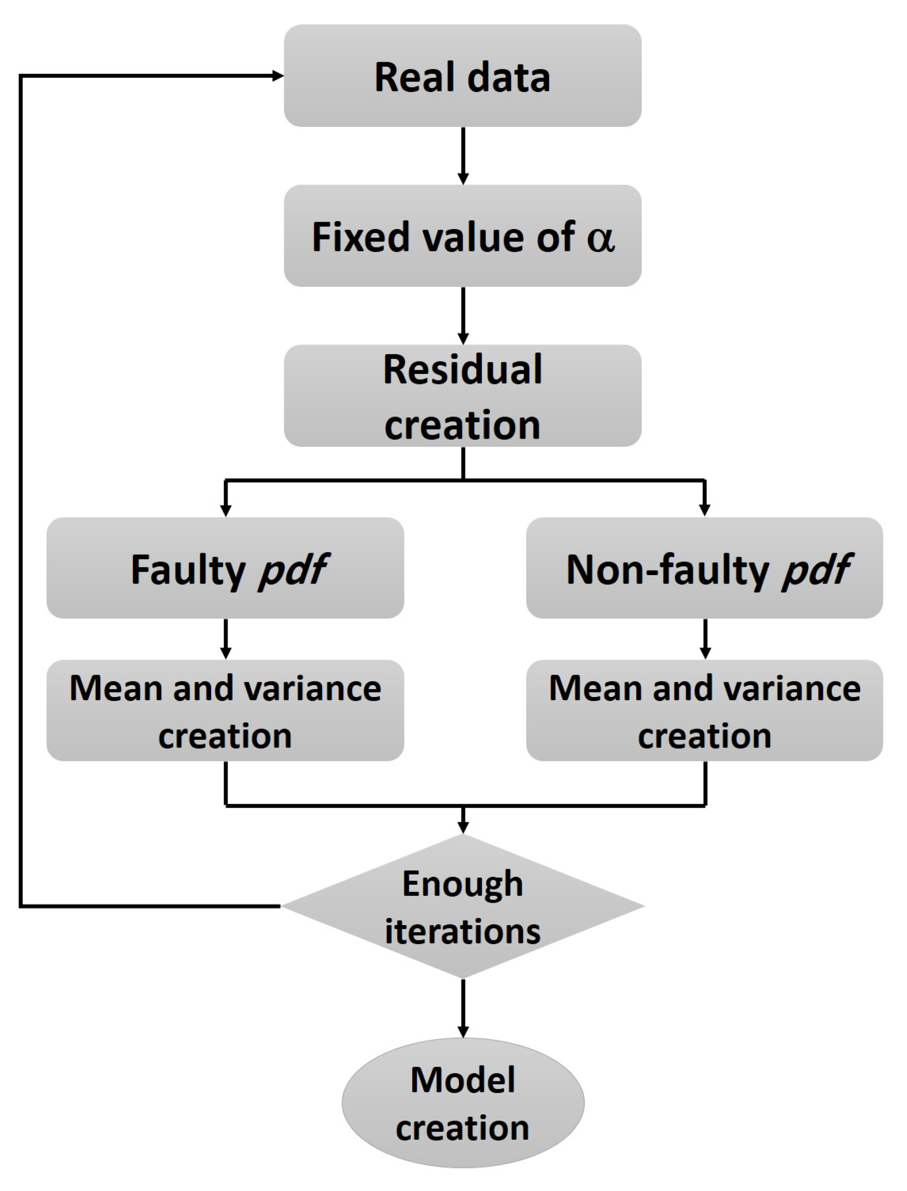
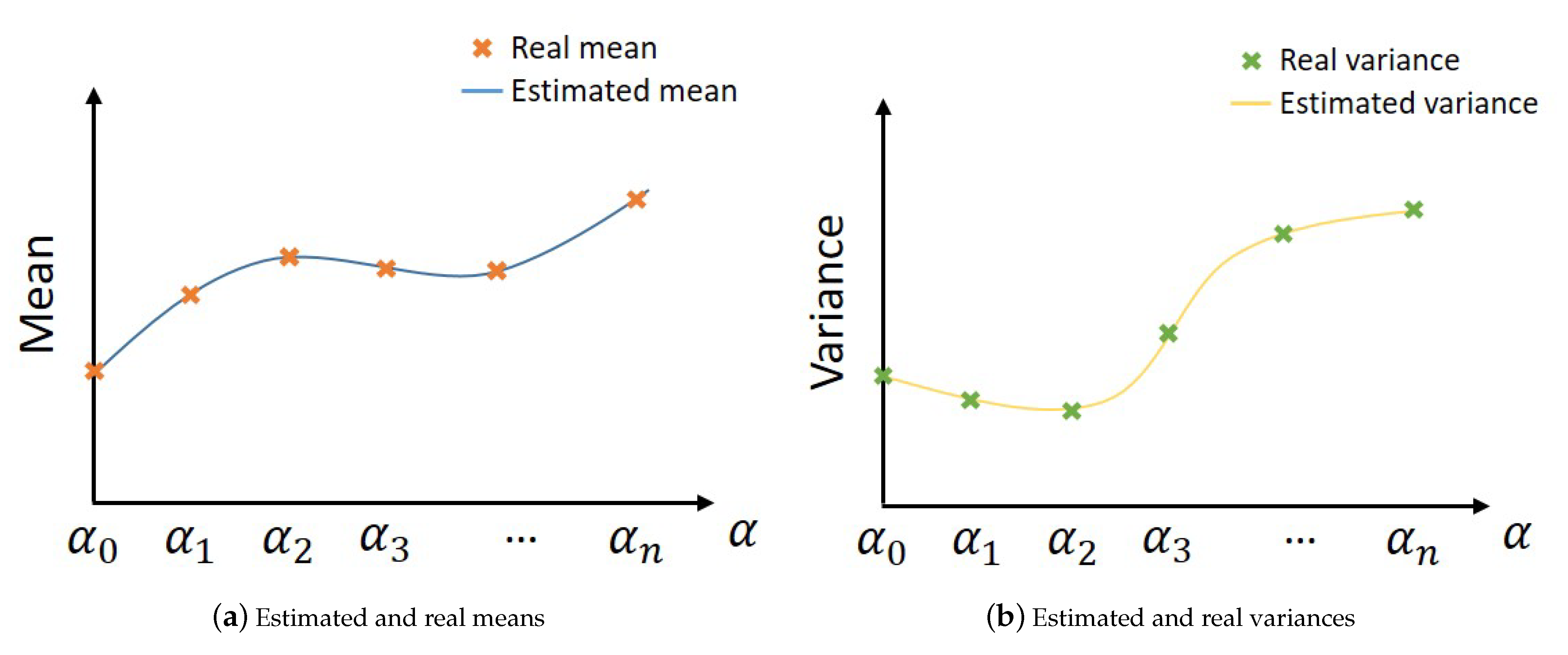
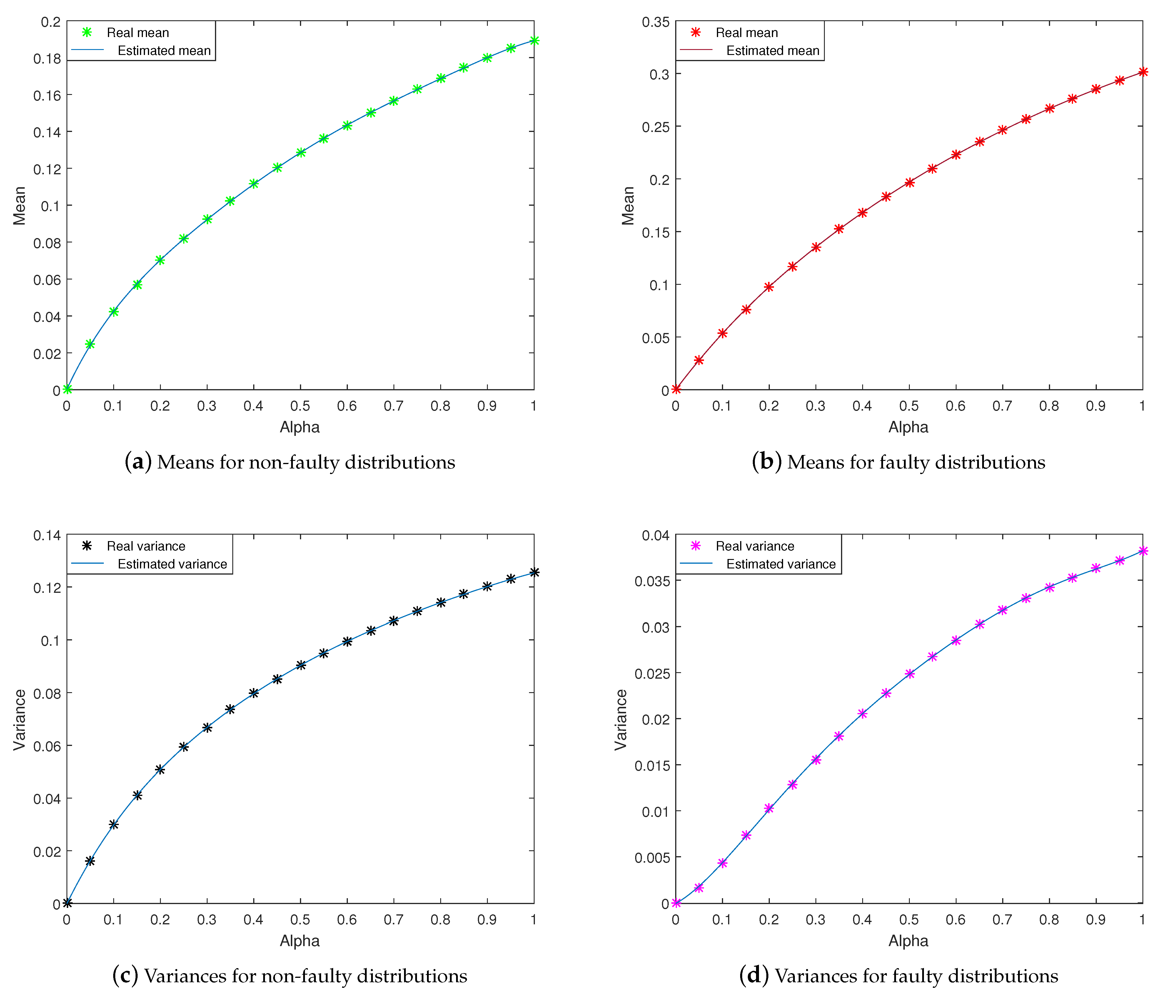
4.3. An Infinity of Residuals Implies an Infinity of Statistical Characterization … How to Solve?
- For non-faulty cases:
- For faulty cases:
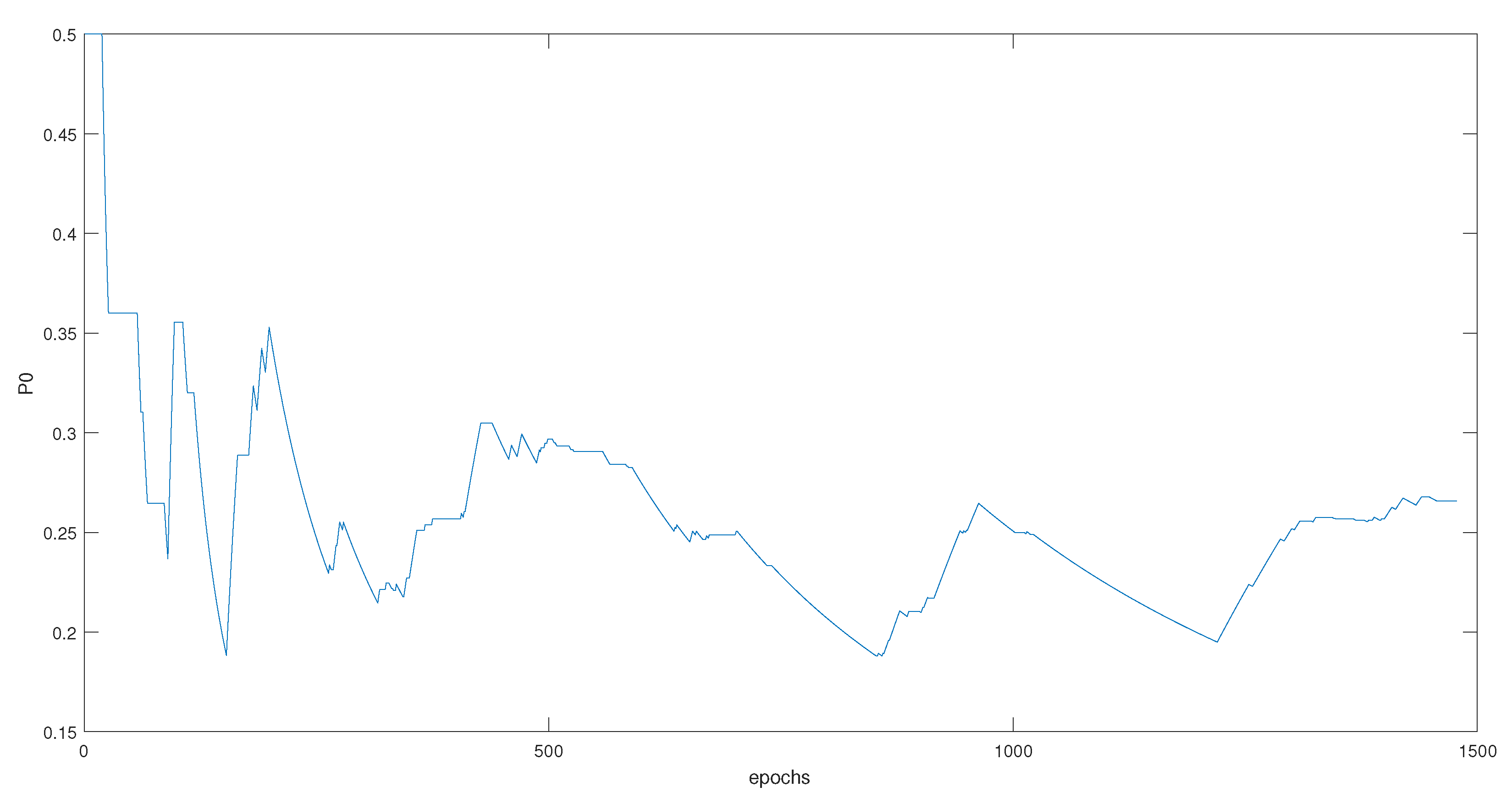
5. -Rényi Criterion Generalizing Threshold Optimization
5.1. -Rc Design
5.2. Variation of -Rc
- for , the derivative of -Rc with respect to is written as:Based on Equation (23):
- if ,
- if ,
- if .
We conclude that -Rc is a decreasing function on and an increasing function on with a minimum point reached at . Hence, by maximizing the -Rc, the is maximized when is fixed. - for , the derivative of -Rc with respect to is written as:Based on Equation (24):
- if ,
- if ,
- if .
We conclude that -Rc is a decreasing function on and an increasing function on with a minimum point reached at . Accordingly, by maximizing the -Rc, the is minimized when is fixed.As conclusion, in order to minimize the false alarm probability and maximize the detection probability, it is equivalent to maximizing the -Rc.
5.3. Threshold Optimization Algorithm
| Algorithm 1: Threshold optimization based on -Rc |
 |
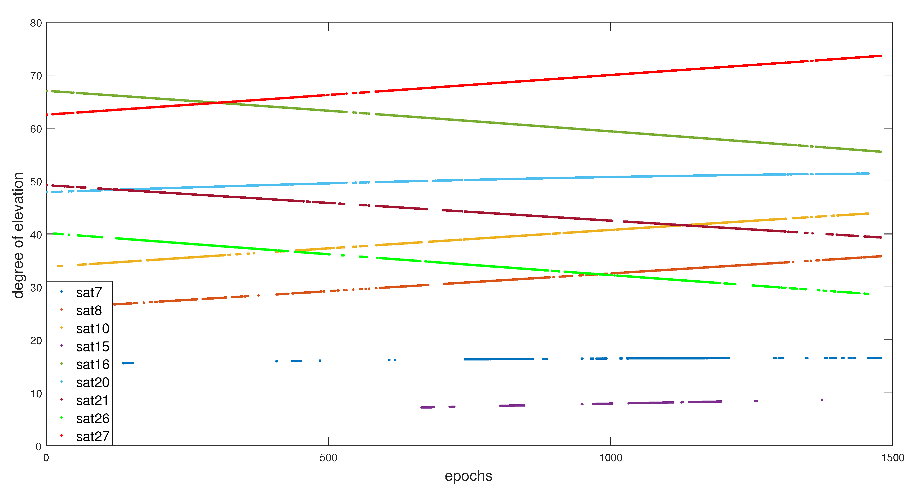
6. Experimental Results
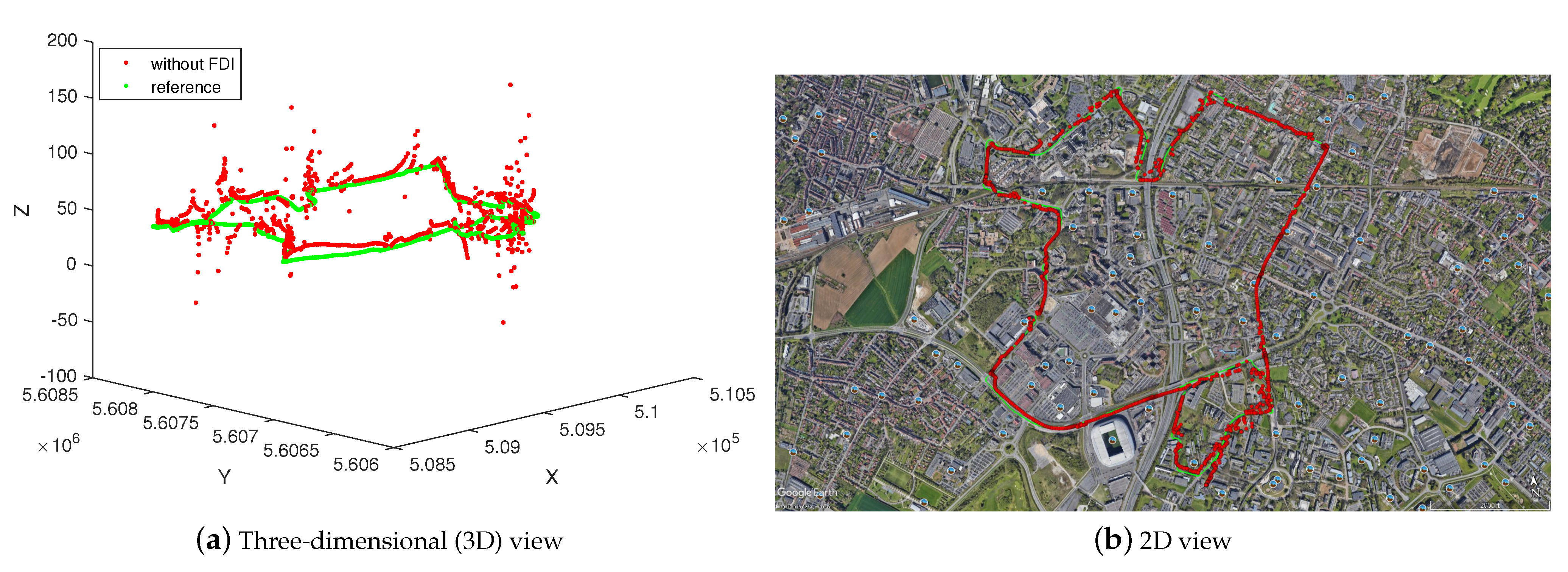
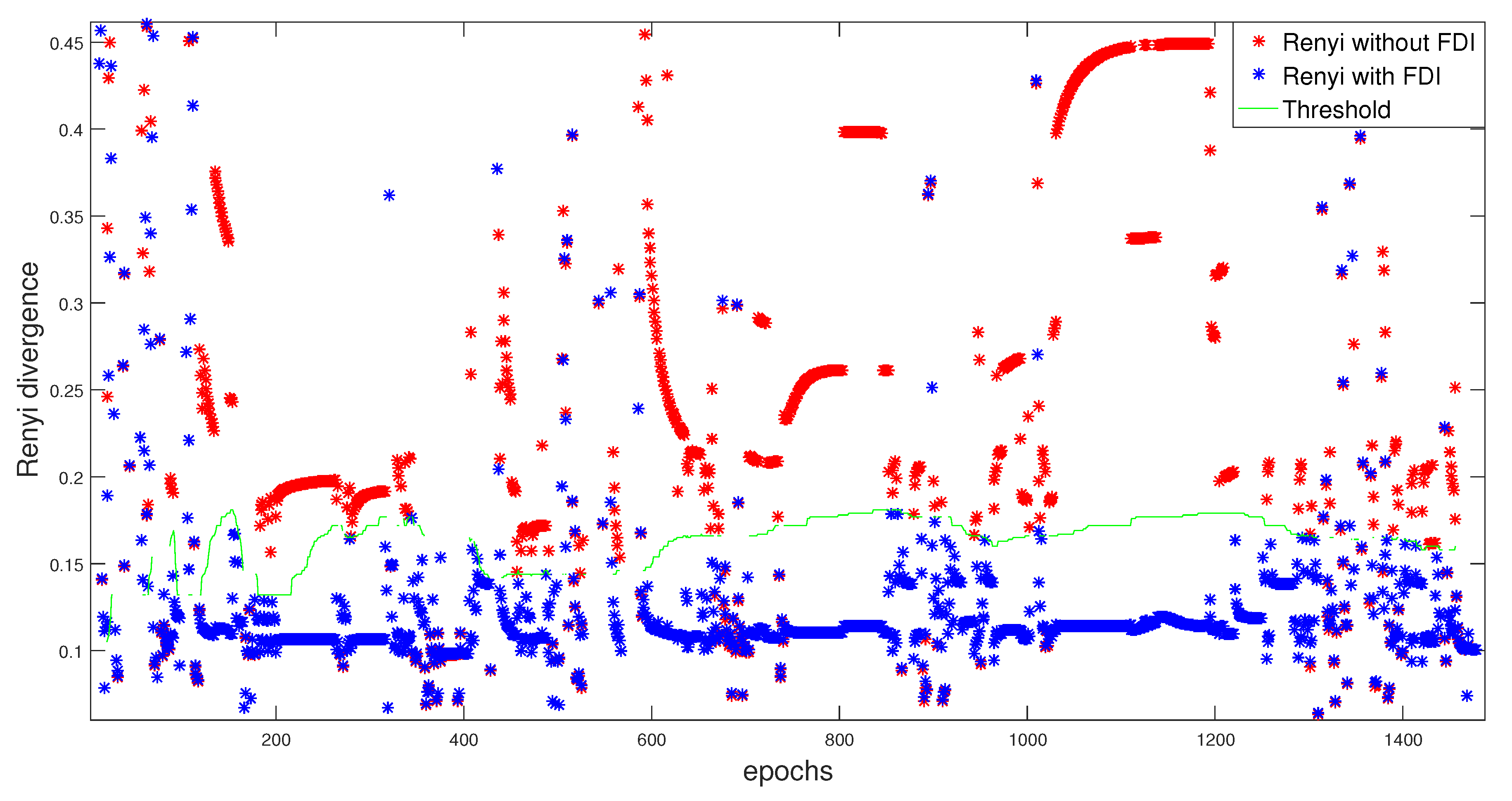
6.1. Results without FDI Approach
6.2. Results with FDI Approach
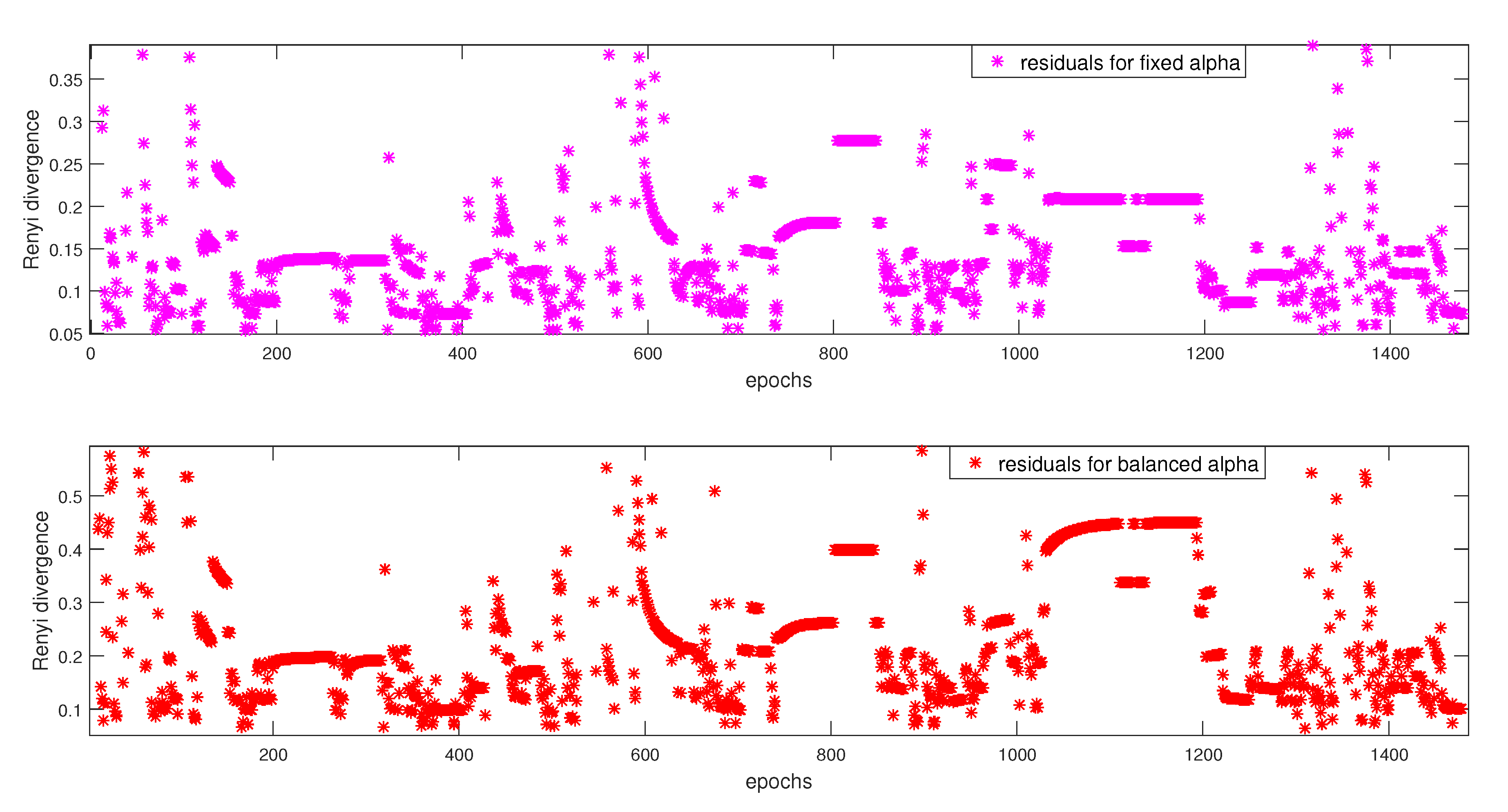
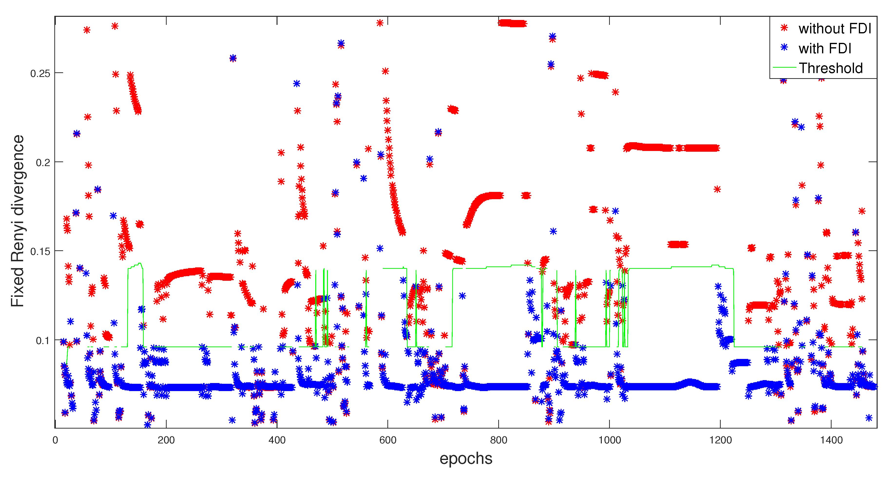
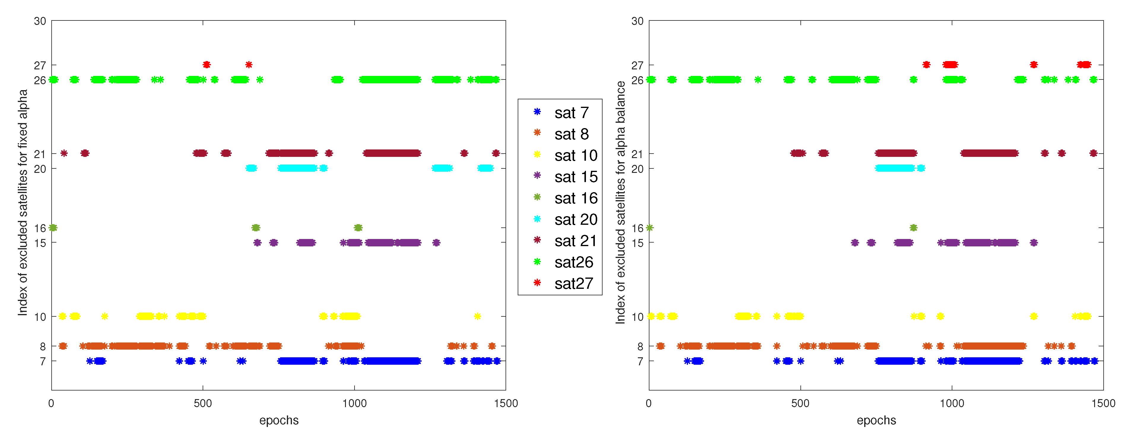
6.2.1. Residual Design Using Fixed
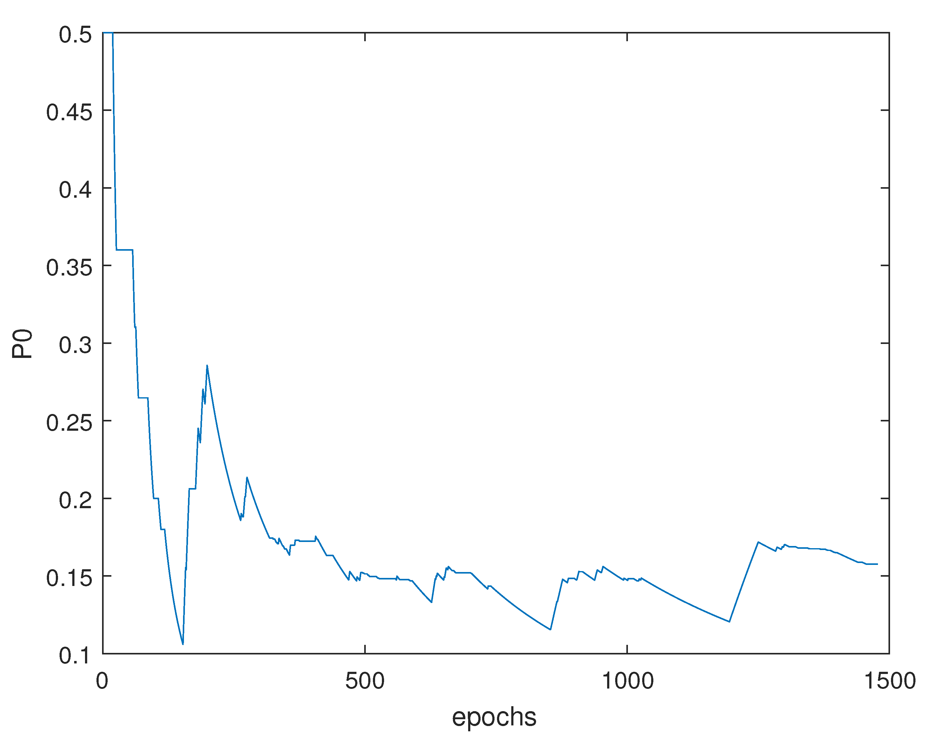
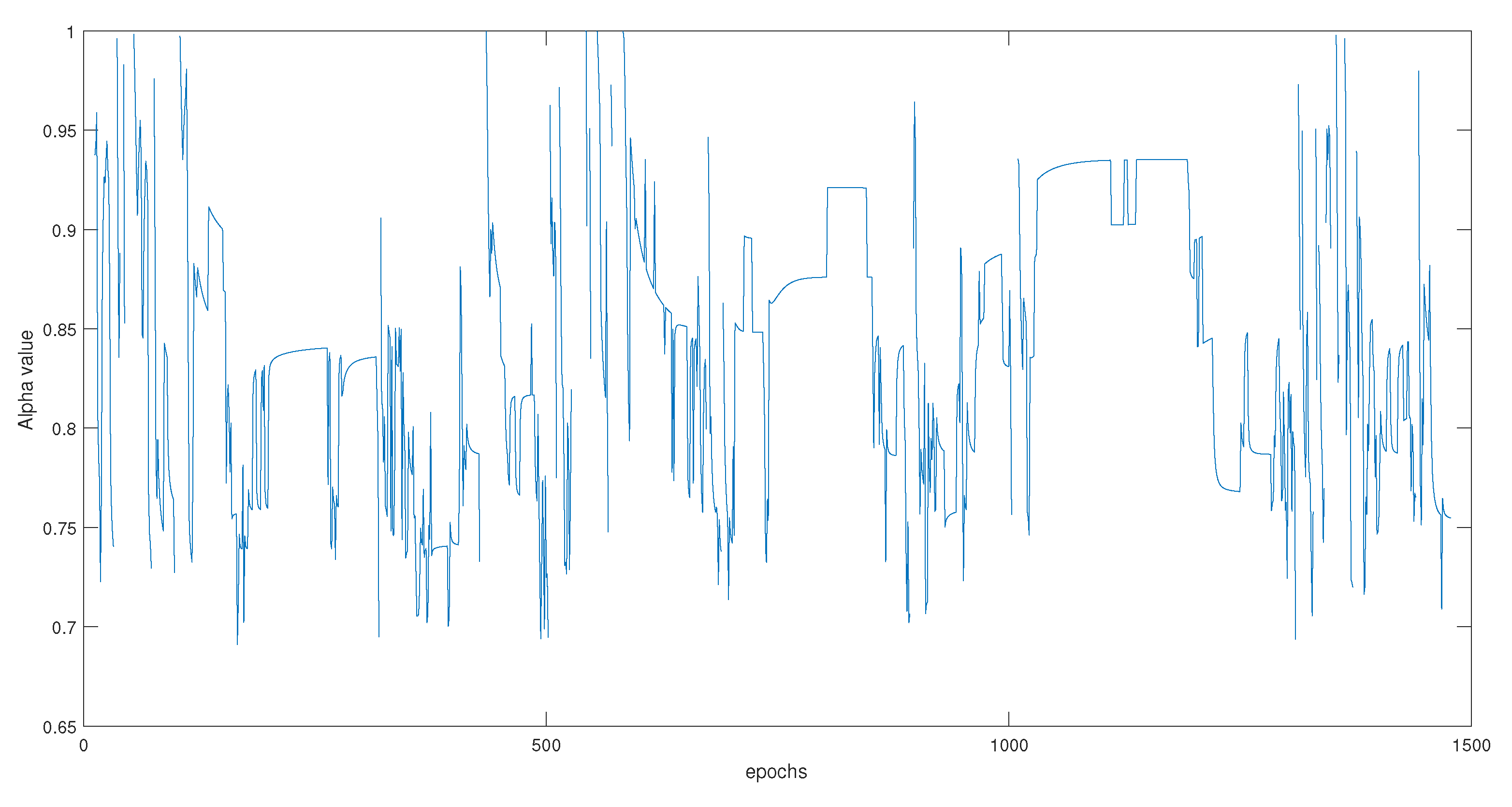
6.2.2. Residual Design Using Balanced
- For non-faulty cases:
- For faulty cases:
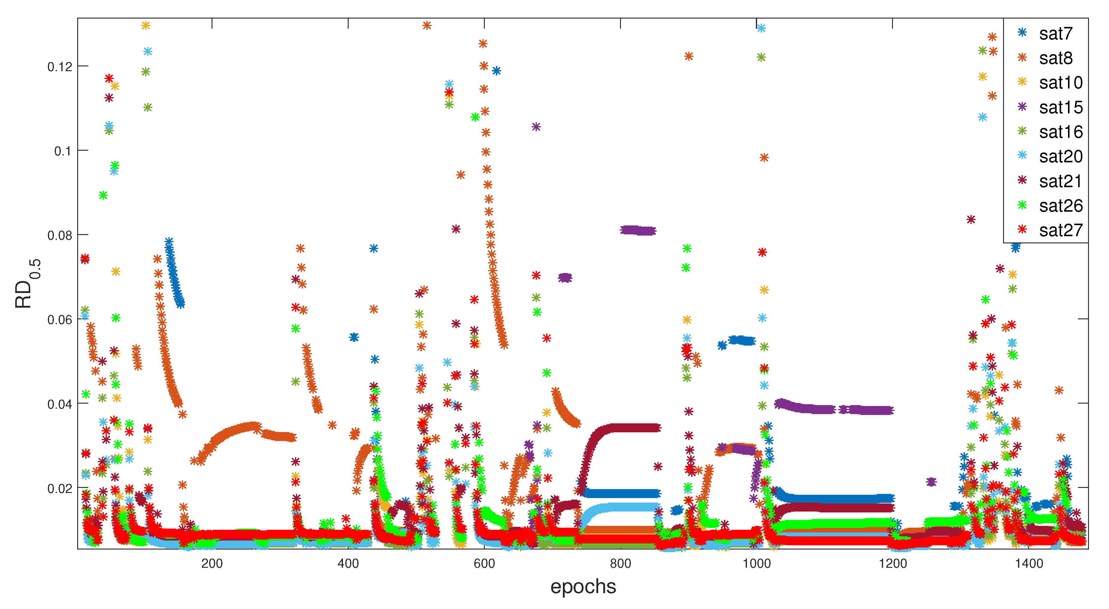
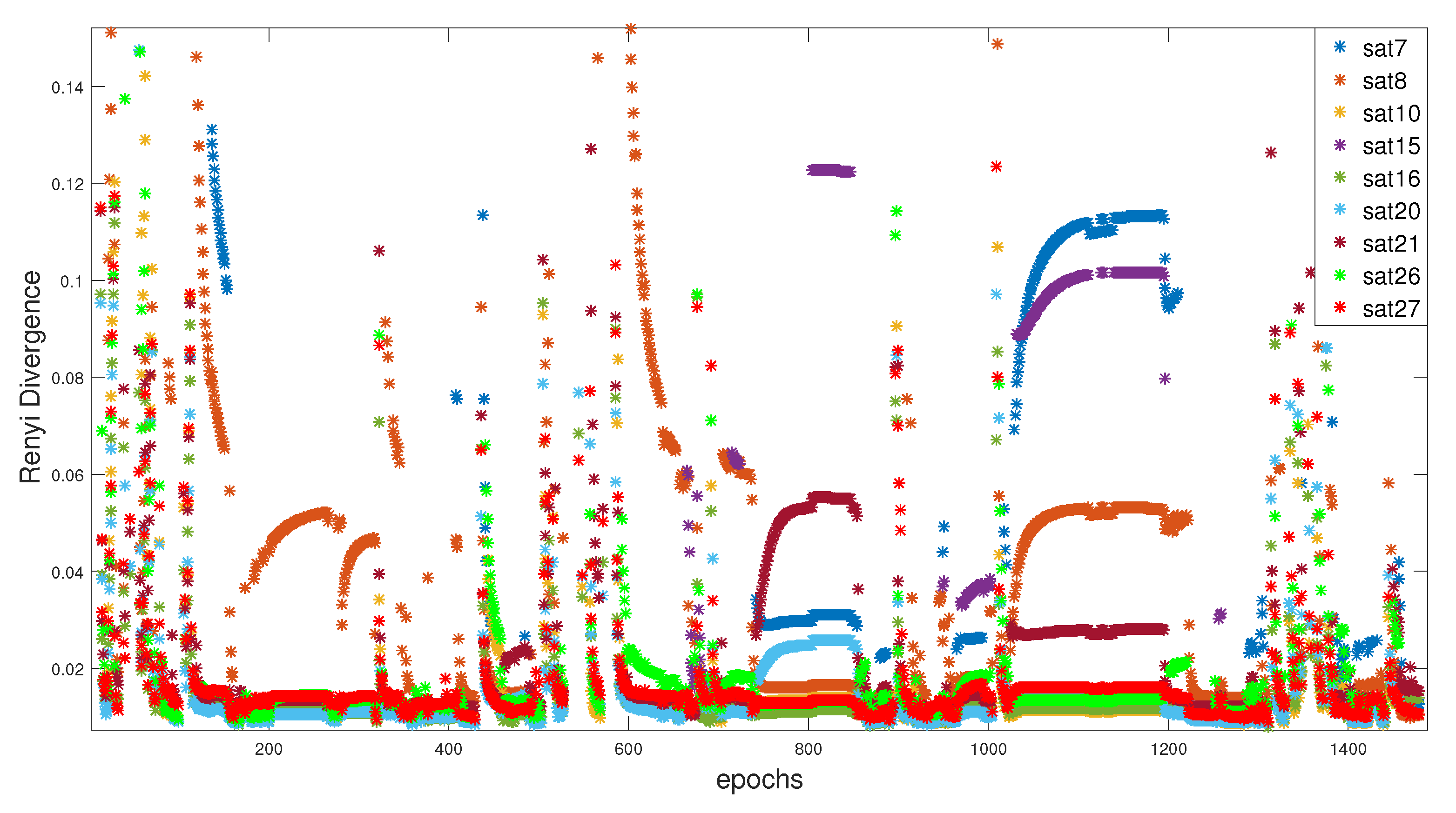
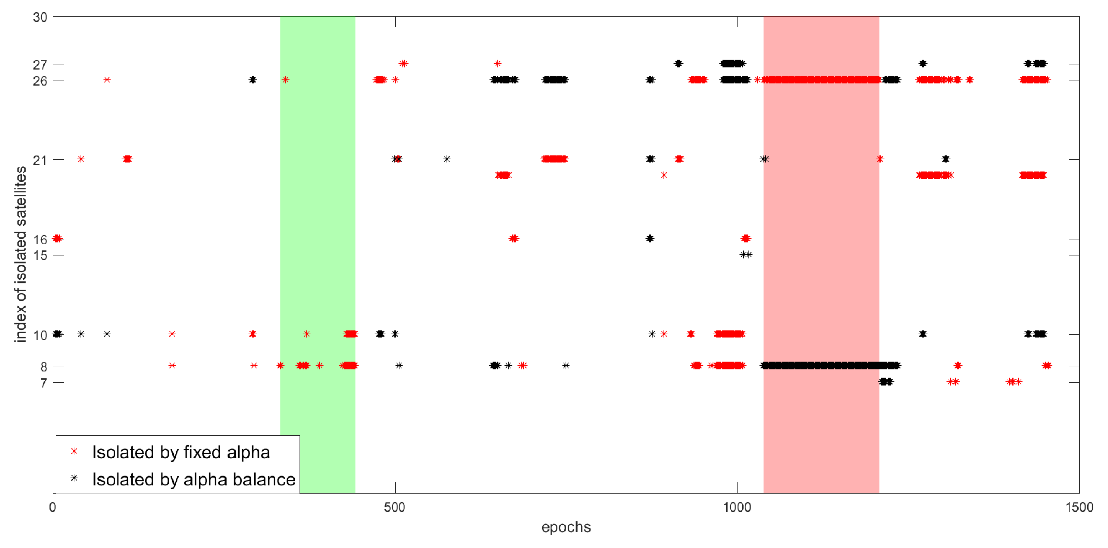
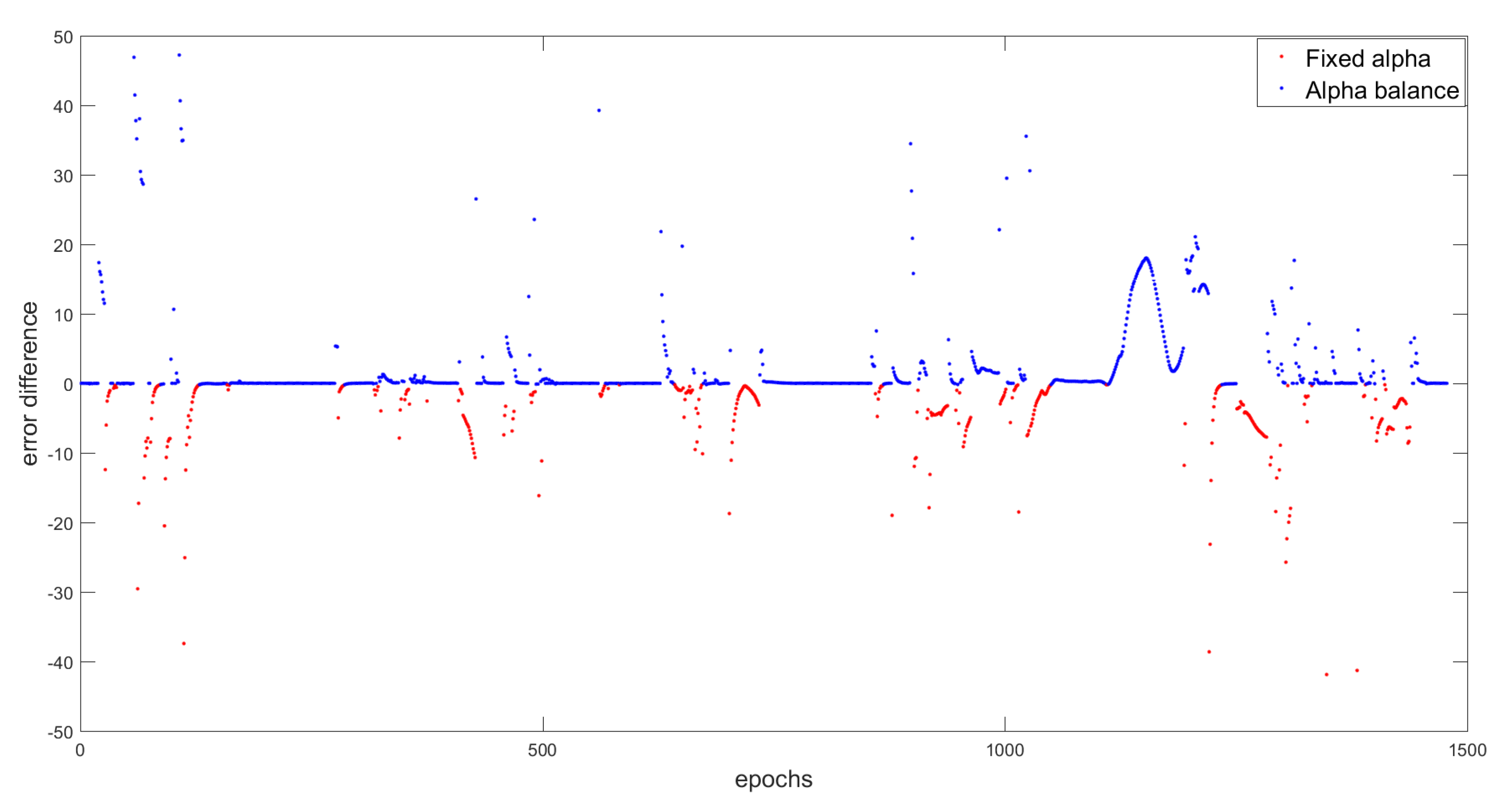
6.2.3. Results Comparison
7. Conclusions
Author Contributions
Funding
Institutional Review Board Statement
Informed Consent Statement
Data Availability Statement
Conflicts of Interest
Abbreviations
| -RD | -Rényi Divergence |
| -Rc | -Rényi criterion |
| ADAS | Advanced Driver Assistance Systems |
| AFTF | Adaptive Fault-Tolerant Fusion |
| AI | Artificial Intelligence |
| CUSUM | CUmulative SUM |
| EKF | Extended Kalman Filter |
| FD | Fault Detection |
| FDI | Fault Detection and Isolation |
| FTF | Fault Tolerant Fusion |
| GNSS | Global Navigation Satellite System |
| IF | Informational Filter |
| IMU | Inertial Measurement Unit |
| INS | Integrated Navigation System |
| ITS | Intelligent Transportation System |
| KF | Kalman Filter |
| KL | Kullback-Leibler |
| KLC | Kullback-Leibler Criterion |
| KLD | Kullback-Leibler divergence |
| KPI | Key Performance Indicator |
| LGPR | Localizing Ground Penetrating Radar |
| MI | Mutual Information |
| NIF | Nonlinear Information Filter |
| NIS | Normalized Innovation Squared |
| NLOS | Non Line-Of-Sight |
| odo | Odometer |
| Probability density functions | |
| PF | Particle Filter |
| QJSD | Quantum Jensen-Shannon divergence |
| SLAM | Simultaneous Localization And Mapping |
| SRR | Short Range Radar |
| SS | Separation Solutions |
| TBM | Transferable Belief Model |
| THR | Tolerable Hazardous Rate |
| UIO | Unknown Input Observers |
Appendix A
References
- National Highway Traffic Safety Administration. Critical reasons for crashes investigated in the national motor vehicle crash causation survey. Wash. DC US Dep. Transp. 2015, 2, 1–2. [Google Scholar]
- Amini, A.; Vaghefi, R.M.; Jesus, M.; Buehrer, R.M. Improving GPS-based vehicle positioning for intelligent transportation systems. In Proceedings of the 2014 IEEE Intelligent Vehicles Symposium Proceedings, Dearborn, MI, USA, 8–11 June 2014; pp. 1023–1029. [Google Scholar]
- Jagadeesh, G.; Srikanthan, T.; Zhang, X. A map matching method for GPS based real-time vehicle location. J. Navig. 2004, 57, 429. [Google Scholar] [CrossRef]
- Brakatsoulas, S.; Pfoser, D.; Salas, R.; Wenk, C. On map-matching vehicle tracking data. In Proceedings of the 31st International Conference on Very Large Data Bases, Trondheim, Norway, 30 August–2 September 2005; pp. 853–864. [Google Scholar]
- Liu, Y.; Liu, F.; Gao, Y.; Zhao, L. Implementation and analysis of tightly coupled global navigation satellite system precise point positioning/inertial navigation system (GNSS PPP/INS) with insufficient satellites for land vehicle navigation. Sensors 2018, 18, 4305. [Google Scholar] [CrossRef] [PubMed]
- Kamijo, S.; Gu, Y.; Hsu, L.T. Autonomous Vehicle Technologies: Localization and Mapping. IEICE ESS Fundam. Rev. 2015, 9, 131–141. [Google Scholar] [CrossRef]
- Ward, E.; Folkesson, J. Vehicle localization with low cost radar sensors. In Proceedings of the 2016 IEEE Intelligent Vehicles Symposium (IV), Gothenburg, Sweden, 19–22 June 2016; pp. 864–870. [Google Scholar]
- Levinson, J.; Montemerlo, M.; Thrun, S. Map-based precision vehicle localization in urban environments. Robot. Sci. Syst. 2007, 4, 1. [Google Scholar]
- Isermann, R. Fault-Diagnosis Systems: An Introduction from Fault Detection to Fault Tolerance; Springer Science & Business Media: Berlin/Heidelberg, Germany, 2006. [Google Scholar]
- Bader, K.; Lussier, B.; Schön, W. A fault tolerant architecture for data fusion: A real application of Kalman filters for mobile robot localization. Robot. Auton. Syst. 2017, 88, 11–23. [Google Scholar] [CrossRef]
- Ricquebourg, V.; Delafosse, M.; Delahoche, L.; Marhic, B.; Jolly-Desodt, A.; Menga, D. Fault detection by combining redundant sensors: A conflict approach within the tbm framework. In Proceedings of the COGIS’07, Stanford, CA, USA, 26–28 November 2007. [Google Scholar]
- Shu-qing, L.; Sheng-xiu, Z. A congeneric multi-sensor data fusion algorithm and its fault-tolerance. In Proceedings of the 2010 International Conference on Computer Application and System Modeling (ICCASM 2010), Taiyuan, China, 22–24 October 2010; Volume 1, p. V1-339. [Google Scholar]
- Allerton, D.J.; Jia, H. Distributed data fusion algorithms for inertial network systems. IET Radar, Sonar Navig. 2008, 2, 51–62. [Google Scholar] [CrossRef]
- Jiang, L. Sensor Fault Detection and Isolation Using System Dynamics Identification Techniques. Ph.D. Thesis, The University of Michigan, Ann Arbor, MI, USA, 2011. [Google Scholar]
- Mehra, R.K.; Peschon, J. An innovations approach to fault detection and diagnosis in dynamic systems. Automatica 1971, 7, 637–640. [Google Scholar] [CrossRef]
- Sundvall, P.; Jensfelt, P. Fault detection for mobile robots using redundant positioning systems. In Proceedings of the 2006 IEEE International Conference on Robotics and Automation (ICRA), Orlando, FL, USA, 15–19 May 2006; pp. 3781–3786. [Google Scholar]
- Morales, Y.; Takeuchi, E.; Tsubouchi, T. Vehicle localization in outdoor woodland environments with sensor fault detection. In Proceedings of the 2008 IEEE International Conference on Robotics and Automation, Pasadena, CA, USA, 19–23 May 2008; pp. 449–454. [Google Scholar]
- Ay, N.; Amari, S.i. A novel approach to canonical divergences within information geometry. Entropy 2015, 17, 8111–8129. [Google Scholar] [CrossRef]
- Shannon, C.E. A mathematical theory of communication. Bell Syst. Tech. J. 1948, 27, 379–423. [Google Scholar] [CrossRef]
- Chen, H.M.; Varshney, P.K.; Arora, M.K. Performance of mutual information similarity measure for registration of multitemporal remote sensing images. IEEE Trans. Geosci. Remote. Sens. 2003, 41, 2445–2454. [Google Scholar] [CrossRef]
- Tmazirte, N.A.; El Najjar, M.E.; Al Hage, J.; Smaili, C.; Pomorski, D. Fast multi fault detection & exclusion approach for GNSS integrity monitoring. In Proceedings of the 17th International Conference on Information Fusion (FUSION), Salamanca, Spain, 7–10 July 2014; pp. 1–6. [Google Scholar]
- Mondal, S.; Chakraborty, G.; Bhattacharyya, K. Robust unknown input observer for nonlinear systems and its application to fault detection and isolation. J. Dyn. Syst. Meas. Control. 2008, 130, 044503. [Google Scholar] [CrossRef]
- Bai, L.; Rossi, L.; Torsello, A.; Hancock, E.R. A quantum Jensen–Shannon graph kernel for unattributed graphs. Pattern Recognit. 2015, 48, 344–355. [Google Scholar] [CrossRef]
- Antolin, J.; Angulo, J.; Lopez-Rosa, S. Fisher and jensen–shannon divergences: Quantitative comparisons among distributions. application to position and momentum atomic densities. J. Chem. Phys. 2009, 130, 074110. [Google Scholar] [CrossRef]
- Radhakrishnan, C.; Parthasarathy, M.; Jambulingam, S.; Byrnes, T. Distribution of quantum coherence in multipartite systems. Phys. Rev. Lett. 2016, 116, 150504. [Google Scholar] [CrossRef]
- De Domenico, M.; Porter, M.A.; Arenas, A. MuxViz: A tool for multilayer analysis and visualization of networks. J. Complex Netw. 2015, 3, 159–176. [Google Scholar] [CrossRef]
- Al Hage, J.; El Najjar, M.E.; Pomorski, D. Multi-sensor fusion approach with fault detection and exclusion based on the Kullback–Leibler Divergence: Application on collaborative multi-robot system. Inf. Fusion 2017, 37, 61–76. [Google Scholar] [CrossRef]
- Basseville, M. Divergence measures for statistical data processing—An annotated bibliography. Signal Process. 2013, 93, 621–633. [Google Scholar] [CrossRef]
- Joerger, M.; Chan, F.C.; Pervan, B. Solution separation versus residual-based RAIM. Navig. J. Inst. Navig. 2014, 61, 273–291. [Google Scholar] [CrossRef]
- Lewandowski, W.; Tisserand, L. Relative characterization of GNSS receiver delays for GPS and GLONASS C/A codes in the L1 frequency band at the OP, SU, PTB and AOS. Bur. Int. Des Poids Mes. Tech. Rep. 2010, 4. [Google Scholar]
- Histace, A.; Rousseau, D. Divergence de Rényi comme mesure de contraste pour la détection d’objets dans des images bruitées. In Proceedings of the GRETSI, Lyon, France, 8–11 September 2015; p. 4. [Google Scholar]
- Van Erven, T.; Harremos, P. Rényi divergence and Kullback-Leibler divergence. IEEE Trans. Inf. Theory 2014, 60, 3797–3820. [Google Scholar] [CrossRef]
- Hobza, T.; Morales, D.; Pardo, L. Rényi statistics for testing equality of autocorrelation coefficients. Stat. Methodol. 2009, 6, 424–436. [Google Scholar] [CrossRef]
- Makkawi, K.; Ait-Tmazirte, N.; El Najjar, M.E.; Moubayed, N. Combination of Maximum Correntropy Criterion & α-Rényi Divergence for a Robust and Fail-Safe Multi-Sensor Data Fusion. In Proceedings of the 2020 IEEE International Conference on Multisensor Fusion and Integration for Intelligent Systems (MFI), Karlsruhe, Germany, 14–16 September 2020; pp. 61–67. [Google Scholar]
- Khoder, M.; Nourdine, A.T.; Nazih, M. Fault Tolerant multi-sensor Data Fusion for vehicle localisation using Maximum Correntropy Unscented Information Filter and α-Rényi Divergence. In Proceedings of the 2020 IEEE 23rd International Conference on Information Fusion (FUSION), Rustenburg, South Africa, 6–9 July 2020; pp. 1–8. [Google Scholar]


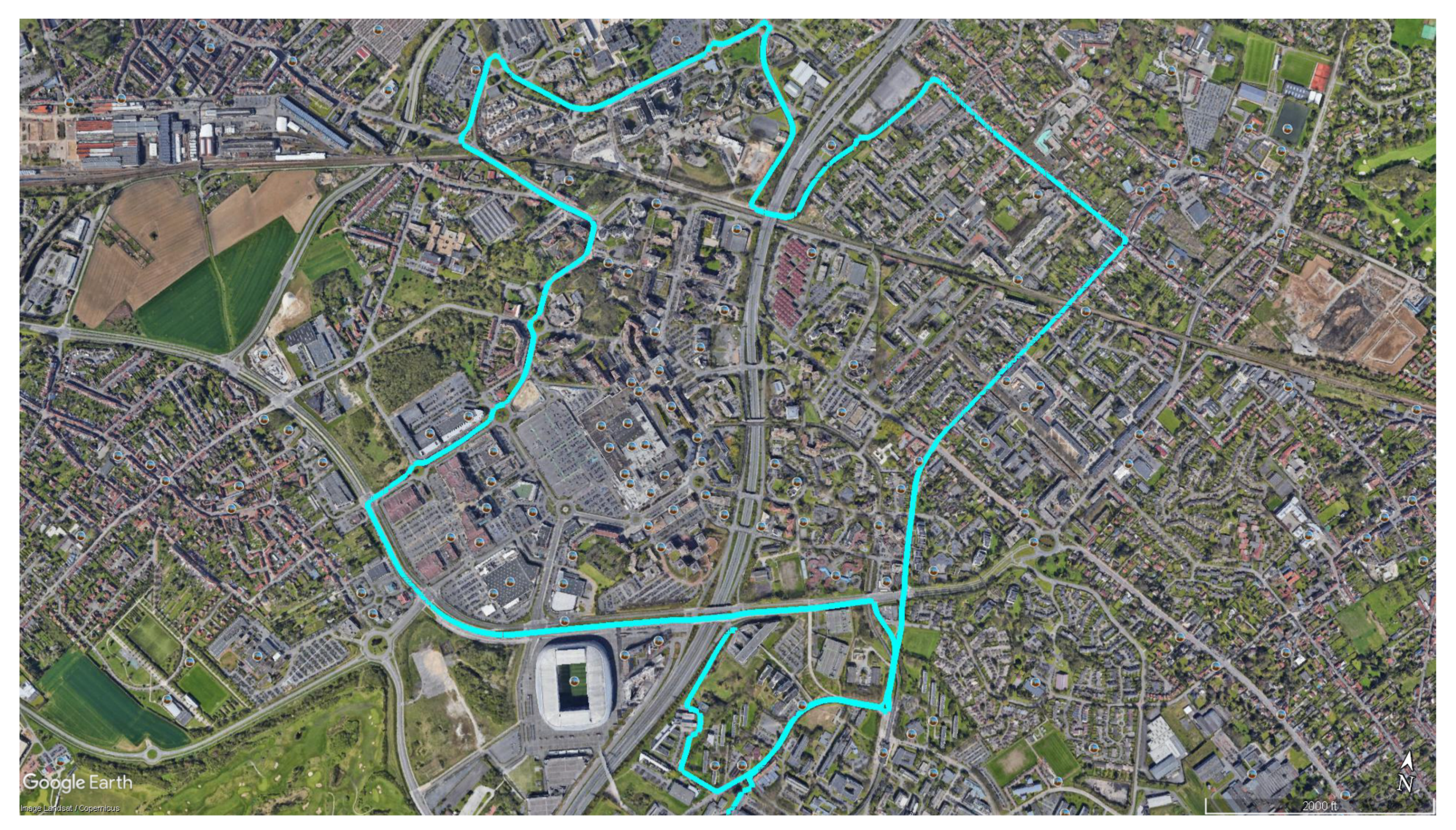
| Trajectory Name | Acquisition Location | Number of Epochs | Trajectory Length |
|---|---|---|---|
| C3 | Villeneuve-d’Ascq | 1477 | 9844.71 m |
| Error Type in Meters | Error Removed by Balance | Error Removed by Fixed | Difference |
|---|---|---|---|
| Mean error | 7.5022 | 6.5306 | 0.9716 |
| Max error | 57.0425 | 51.6895 | 5.3530 |
Publisher’s Note: MDPI stays neutral with regard to jurisdictional claims in published maps and institutional affiliations. |
© 2021 by the authors. Licensee MDPI, Basel, Switzerland. This article is an open access article distributed under the terms and conditions of the Creative Commons Attribution (CC BY) license (https://creativecommons.org/licenses/by/4.0/).
Share and Cite
Makkawi, K.; Ait-Tmazirte, N.; El Badaoui El Najjar, M.; Moubayed, N. Adaptive Diagnosis for Fault Tolerant Data Fusion Based on α-Rényi Divergence Strategy for Vehicle Localization. Entropy 2021, 23, 463. https://doi.org/10.3390/e23040463
Makkawi K, Ait-Tmazirte N, El Badaoui El Najjar M, Moubayed N. Adaptive Diagnosis for Fault Tolerant Data Fusion Based on α-Rényi Divergence Strategy for Vehicle Localization. Entropy. 2021; 23(4):463. https://doi.org/10.3390/e23040463
Chicago/Turabian StyleMakkawi, Khoder, Nourdine Ait-Tmazirte, Maan El Badaoui El Najjar, and Nazih Moubayed. 2021. "Adaptive Diagnosis for Fault Tolerant Data Fusion Based on α-Rényi Divergence Strategy for Vehicle Localization" Entropy 23, no. 4: 463. https://doi.org/10.3390/e23040463
APA StyleMakkawi, K., Ait-Tmazirte, N., El Badaoui El Najjar, M., & Moubayed, N. (2021). Adaptive Diagnosis for Fault Tolerant Data Fusion Based on α-Rényi Divergence Strategy for Vehicle Localization. Entropy, 23(4), 463. https://doi.org/10.3390/e23040463