
RF Signal-Based UAV Detection and Mode Classification: A Joint Feature Engineering Generator and Multi-Channel Deep Neural Network Approach


Abstract
:1. Introduction
- We design a joint FEG and MC-DNN approach for UAV detection and mode classification. The RF signals are preprocessed by FEG and then input into an MC-DNN for classification.
- In FEG, data truncation and normalization separates different components, the moving average filter removes the noise in the signals, and the concatenation exploits comprehensive details of the RF samples.
- We design MC-DNN to classify the signals preprocessed by the proposed FEG. The multi-channel input separates different frequency components of data to reduce interferences, and MC-DNN learns the classification effectively.
- We verify the joint approach through extensive experiments on an open dataset consisting of ten RF signal categories from three types of UAVs. Our method achieves high accuracy and F1 score and outperforms other methods.
2. Related Works
3. System Model and Problems
3.1. System Model
3.1.1. RF Signal Acquisition
3.1.2. Noise and Interference in RF Signals
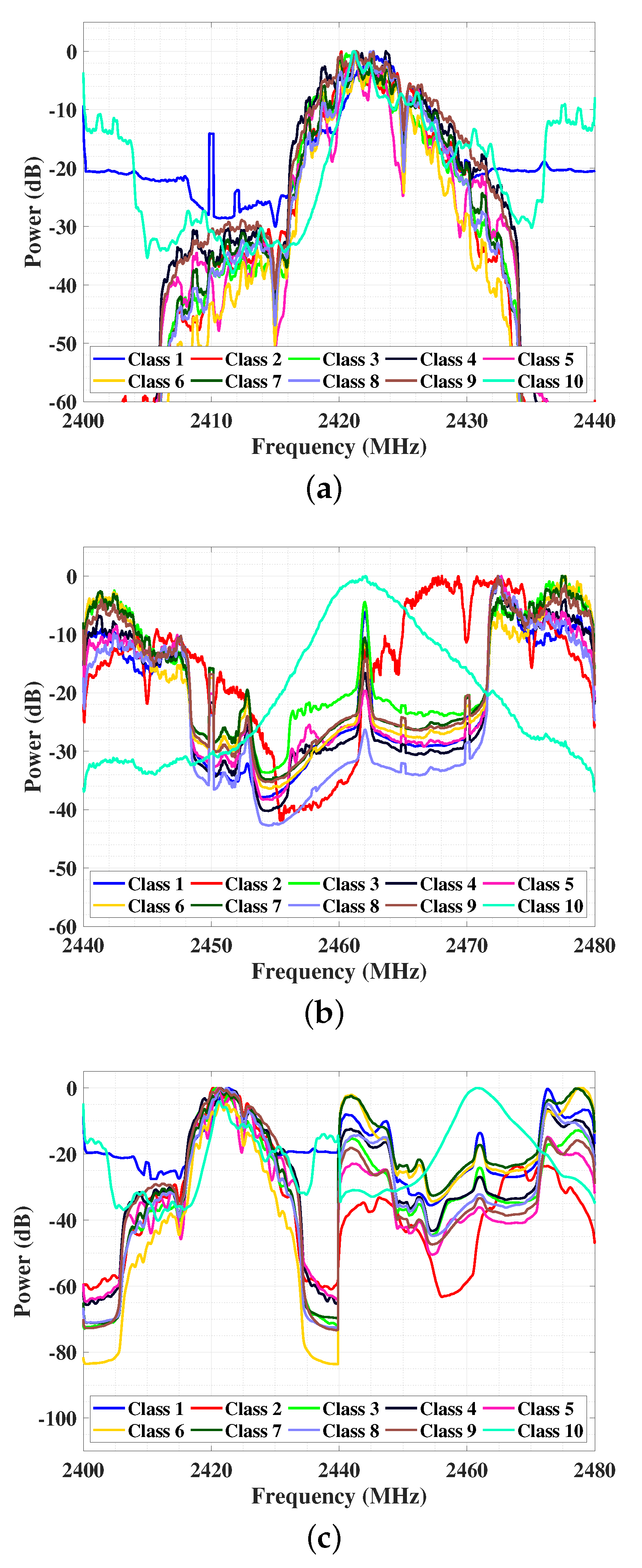
3.1.3. RF Signals in Frequency Domain
3.2. Problems
4. Methodology
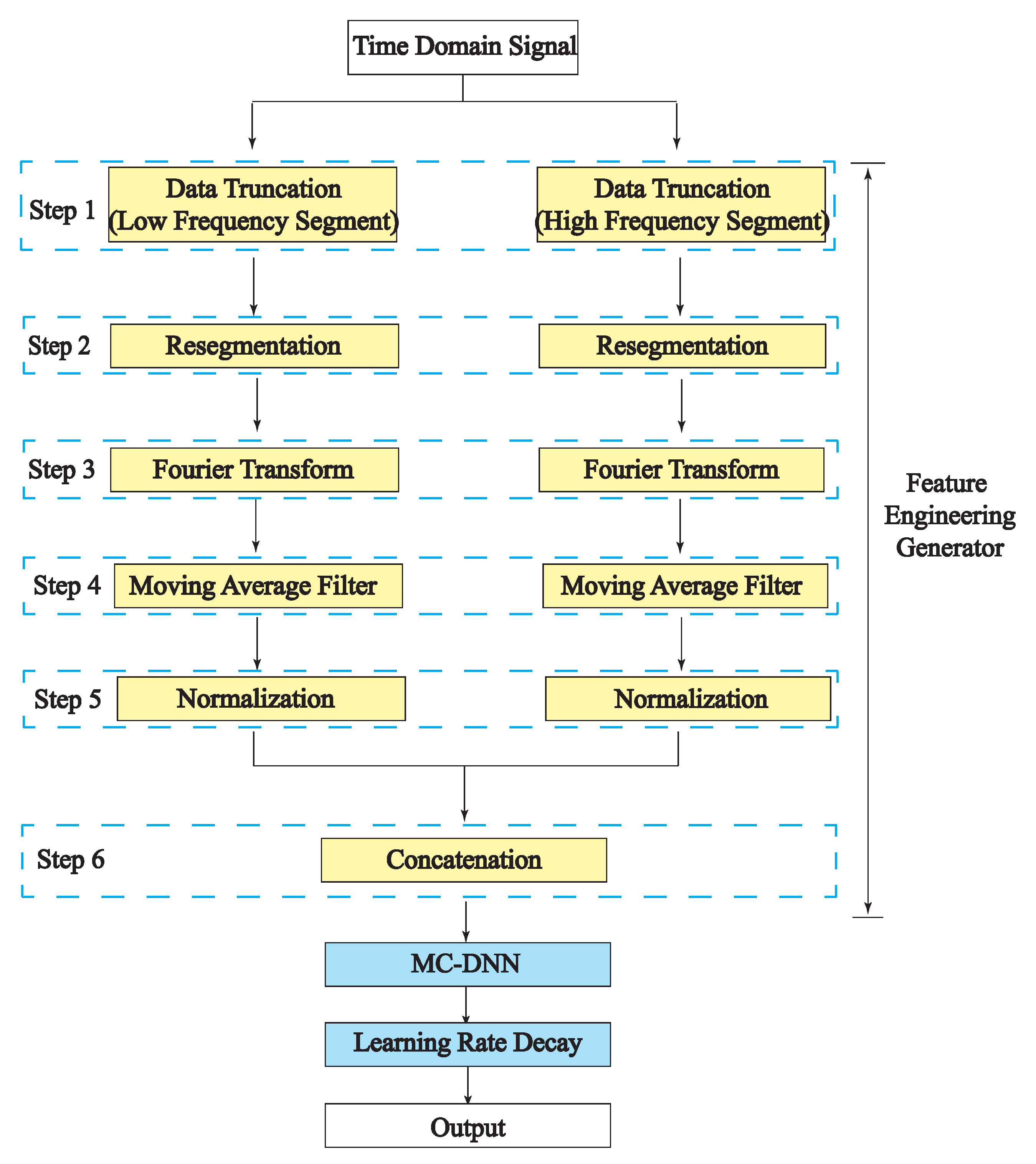
4.1. Feature Engineering Generator
4.1.1. Data Truncation and Normalization
4.1.2. Moving Average Filter
4.1.3. Concatenation
| Algorithm 1 Feature Engineering Generator Algorithm. |
Require:
The Feature Engineering Generator preprocessed frequency domain data D.
|
4.2. DNN Structure
4.2.1. Deep Neural Network
Input and Objective
Deep Neural Network Structure
Loss Function
Stratified K-Fold Cross-Validation
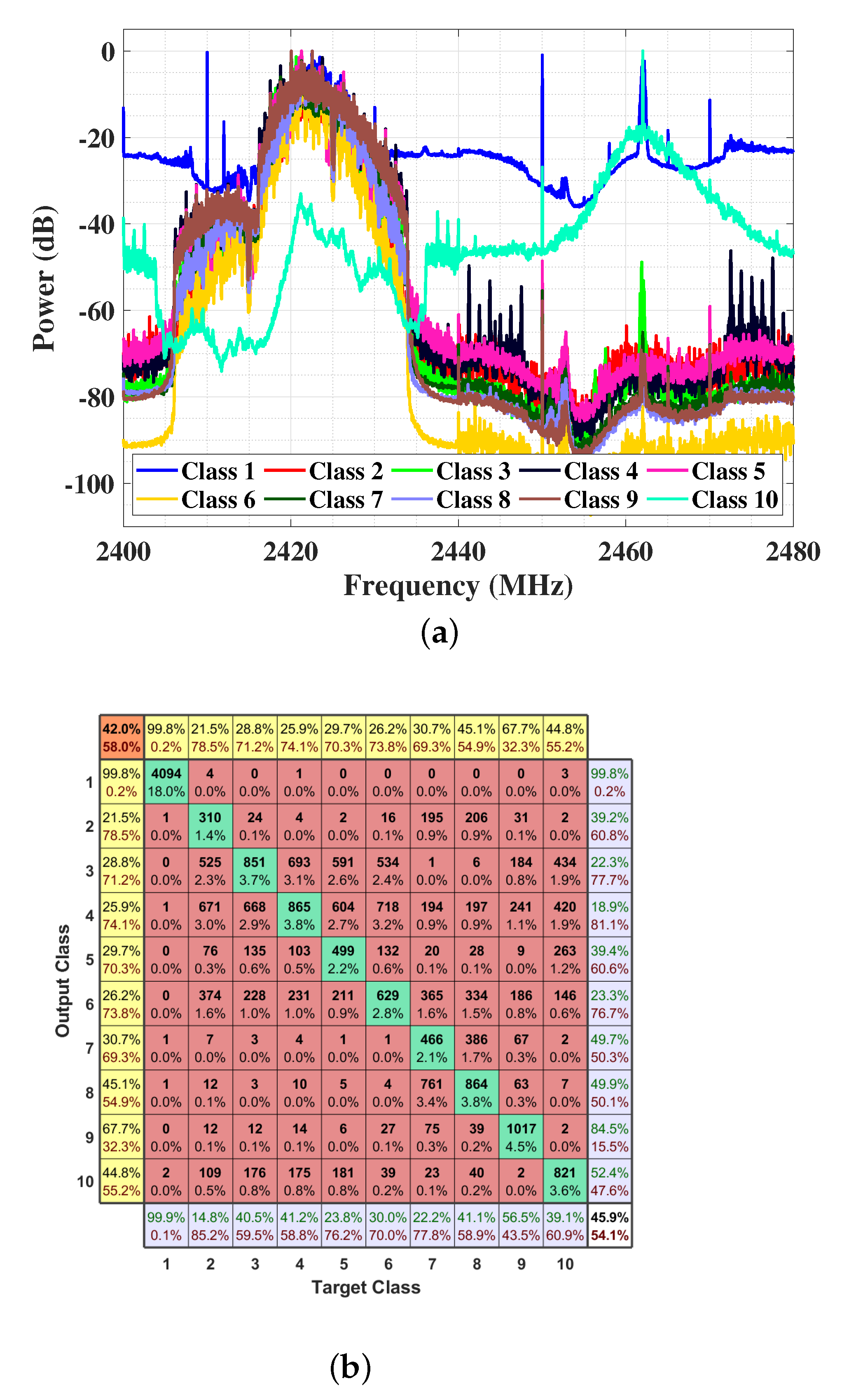
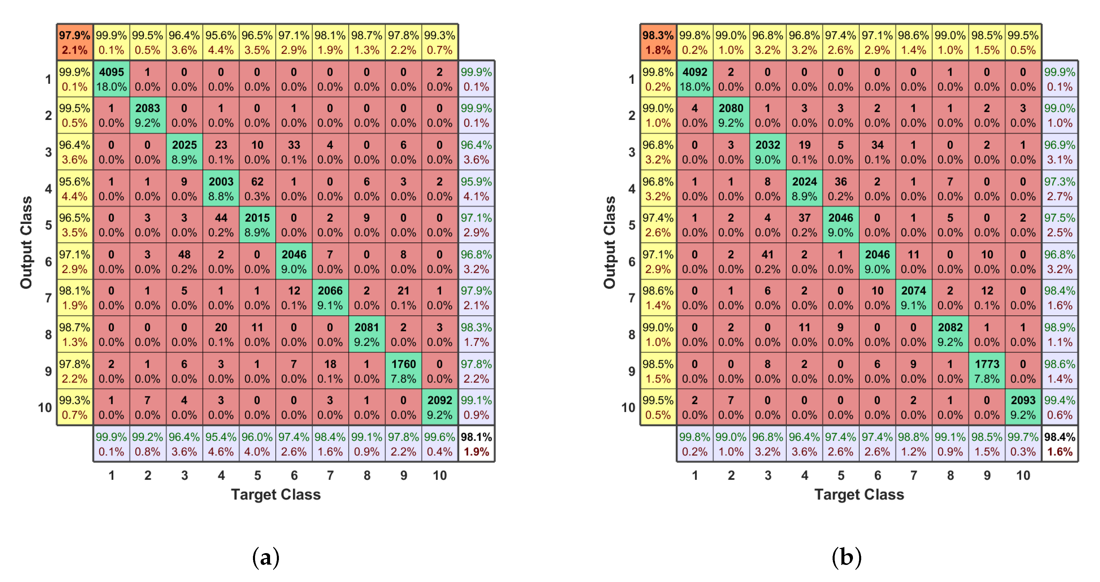
Confusion Matrix
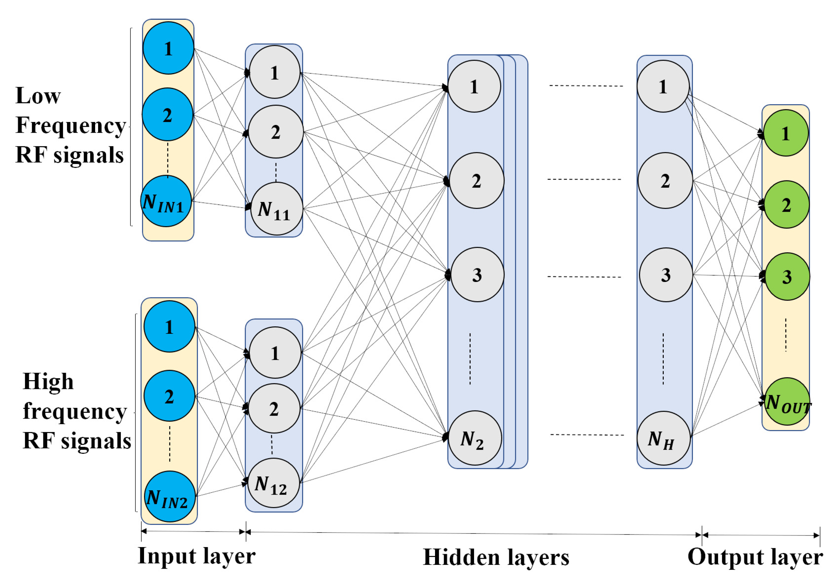
4.2.2. Multi-Channel DNN
4.2.3. Learning Rate Decay
5. Experiments
5.1. Dataset
5.2. DNN
5.3. Joint DNN and Feature Engineering Generator
5.3.1. Data Truncation and Normalization
5.3.2. Moving Average Filter
5.3.3. Concatenation
5.4. Joint MC-DNN and Feature Engineering Generator
5.4.1. Multi-Channel Input
5.4.2. Learning Rate Decay
5.5. Comparison
6. Conclusions
Author Contributions
Funding
Institutional Review Board Statement
Informed Consent Statement
Data Availability Statement
Conflicts of Interest
Abbreviations
| UAV | Unmanned Aerial Vehicle |
| RF | Radio Frequency |
| FEG | Feature Engineering Generator |
| DNN | Deep Neural Network |
| MC-DNN | Multi-Channel Deep Neural Network |
| CNN | Convolutional Neural Network |
| NCA | neighborhood component analysis |
| RADAR | Radio detection and ranging |
| SNR | Signal-to-noise Ratio |
| SINR | Signal to Interference plus Noise Ratio |
| USRP | Universal Software Radio Peripheral |
| ReLU | rectified linear Unit Function |
| 1D | One Dimentional |
| FDR | False Discovery Rate |
| FNR | False-Negative Rate |
References
- Zhao, N.; Lu, W.; Sheng, M.; Chen, Y.; Tang, J.; Yu, F.R.; Wong, K. UAV-Assisted Emergency Networks in Disasters. IEEE Wirel. Commun. 2019, 26, 45–51. [Google Scholar] [CrossRef] [Green Version]
- Ullah, S.; Kim, K.I.; Kim, K.H.; Imran, M.; Khan, P.; Tovar, E.; Ali, F. UAV-enabled healthcare architecture: Issues and challenges. Future Gener. Comput. Syst. 2019, 97, 425–432. [Google Scholar] [CrossRef]
- Singh, A.; Patil, D.; Omkar, S. Eye in the Sky: Real-Time Drone Surveillance System (DSS) for Violent Individuals Identification Using ScatterNet Hybrid Deep Learning Network. In Proceedings of the IEEE Conference on Computer Vision and Pattern Recognition Workshops, Salt Lake City, UT, USA, 18–22 June 2018. [Google Scholar]
- Drummond, C.D.; Harley, M.D.; Turner, I.L.; AMatheen, A.N.; Glamore, W.C. UAV applications to coastal engineering. In Proceedings of the Australasian Coasts & Ports Conference 2015: 22nd Australasian Coastal and Ocean Engineering Conference and the 15th Australasian Port and Harbour Conference, Engineers Australia and IPENZ, Auckland, New Zealand, 15–18 September 2015; p. 267. [Google Scholar]
- Menouar, H.; Guvenc, I.; Akkaya, K.; Uluagac, A.S.; Kadri, A.; Tuncer, A. UAV-Enabled Intelligent Transportation Systems for the Smart City: Applications and Challenges. IEEE Commun. Mag. 2017, 55, 22–28. [Google Scholar] [CrossRef]
- Lygouras, E.; Gasteratos, A.; Tarchanidis, K.; Mitropoulos, A.C. ROLFER: A fully autonomous aerial rescue support system. Microprocess. Microsyst. 2018, 61, 32–42. [Google Scholar] [CrossRef]
- Idries, A.; Mohamed, N.; Jawhar, I.; Mohamed, F.; Al-Jaroodi, J. Challenges of developing UAV applications: A project management view. In Proceedings of the 2015 International Conference on Industrial Engineering and Operations Management (IEOM), Dubai, United Arab Emirates, 3–5 March 2015; pp. 1–10. [Google Scholar] [CrossRef]
- Zeng, Y.; Zhang, R.; Lim, T.J. Wireless communications with unmanned aerial vehicles: Opportunities and challenges. IEEE Commun. Mag. 2016, 54, 36–42. [Google Scholar] [CrossRef] [Green Version]
- Zeng, Y.; Zhang, R. Energy-Efficient UAV Communication With Trajectory Optimization. IEEE Trans. Wirel. Commun. 2017, 16, 3747–3760. [Google Scholar] [CrossRef] [Green Version]
- Luong, P.; Gagnon, F.; Tran, L.N.; Labeau, F. Deep Reinforcement Learning Based Resource Allocation in Cooperative UAV-Assisted Wireless Networks. IEEE Trans. Wirel. Commun. 2021, 20, 7610–7625. [Google Scholar] [CrossRef]
- Li, B.; Zhao, S.; Zhang, R.; Yang, L. Full-Duplex UAV Relaying for Multiple User Pairs. IEEE Internet Things J. 2021, 8, 4657–4667. [Google Scholar] [CrossRef]
- Horapong, K.; Chandrucka, D.; Montree, N.; Buaon, P. Design and use of “Drone” to support the radio navigation aids flight inspection. In Proceedings of the 2017 IEEE/AIAA 36th Digital Avionics Systems Conference (DASC), St. Petersburg, FL, USA, 17–21 September 2017; pp. 1–6. [Google Scholar]
- Sekander, S.; Tabassum, H.; Hossain, E. Multi-Tier Drone Architecture for 5 G/B5 G Cellular Networks: Challenges, Trends, and Prospects. IEEE Commun. Mag. 2018, 56, 96–103. [Google Scholar] [CrossRef] [Green Version]
- Gupta, L.; Jain, R.; Vaszkun, G. Survey of Important Issues in UAV Communication Networks. IEEE Commun. Surv. Tutor. 2016, 18, 1123–1152. [Google Scholar] [CrossRef] [Green Version]
- Nassi, B.; Shabtai, A.; Masuoka, R.; Elovici, Y. SoK—Security and Privacy in the Age of Drones: Threats, Challenges, Solution Mechanisms, and Scientific Gaps. arXiv 2019, arXiv:1903.05155. [Google Scholar]
- Zhi, Y.; Fu, Z.; Sun, X.; Yu, J. Security and privacy issues of UAV: A survey. Mob. Networks Appl. 2020, 25, 95–101. [Google Scholar] [CrossRef]
- Güvenç, I.; Ozdemir, O.; Yapici, Y.; Mehrpouyan, H.; Matolak, D. Detection, localization, and tracking of unauthorized UAS and Jammers. In Proceedings of the 2017 IEEE/AIAA 36th Digital Avionics Systems Conference (DASC), St. Petersburg, FL, USA, 17–21 September 2017; pp. 1–10. [Google Scholar] [CrossRef]
- Ganti, S.R.; Kim, Y. Implementation of detection and tracking mechanism for small UAS. In Proceedings of the 2016 International Conference on Unmanned Aircraft Systems (ICUAS), Arlington, VA, USA, 7–10 June 2016; pp. 1254–1260. [Google Scholar] [CrossRef]
- Ezuma, M.; Erden, F.; Kumar Anjinappa, C.; Ozdemir, O.; Guvenc, I. Detection and Classification of UAVs Using RF Fingerprints in the Presence of Wi-Fi and Bluetooth Interference. IEEE Open J. Commun. Soc. 2020, 1, 60–76. [Google Scholar] [CrossRef]
- Ezuma, M.; Erden, F.; Anjinappa, C.K.; Ozdemir, O.; Guvenc, I. Micro-UAV Detection and Classification from RF Fingerprints Using Machine Learning Techniques. In Proceedings of the 2019 IEEE Aerospace Conference, Big Sky, MT, USA, 2–9 March 2019; pp. 1–13. [Google Scholar]
- Bhattacherjee, U.; Ozturk, E.; Ozdemir, O.; Guvenc, I.; Sichitiu, M.L.; Dai, H. Experimental Study of Outdoor UAV Localization and Tracking using Passive RF Sensing. arXiv 2021, arXiv:2108.07857. [Google Scholar]
- Al-Sa’d, M.F.; Al-Ali, A.; Mohamed, A.; Khattab, T.; Erbad, A. RF-based drone detection and identification using deep learning approaches: An initiative towards a large open source drone database. Future Gener. Comput. Syst. 2019, 100, 86–97. [Google Scholar] [CrossRef]
- Al-Emadi, S.; Al-Senaid, F. Drone Detection Approach Based on Radio-Frequency Using Convolutional Neural Network. In Proceedings of the 2020 IEEE International Conference on Informatics, IoT, and Enabling Technologies (ICIoT), Doha, Qatar, 2–5 February 2020; pp. 29–34. [Google Scholar] [CrossRef]
- Allahham, M.S.; Khattab, T.; Mohamed, A. Deep Learning for RF-Based Drone Detection and Identification: A Multi-Channel 1-D Convolutional Neural Networks Approach. In Proceedings of the 2020 IEEE International Conference on Informatics, IoT, and Enabling Technologies (ICIoT), Doha, Qatar, 2–5 February 2020; pp. 112–117. [Google Scholar] [CrossRef]
- Moses, A.; Rutherford, M.J.; Valavanis, K.P. Radar-based detection and identification for miniature air vehicles. In Proceedings of the 2011 IEEE International Conference on Control Applications (CCA), Denver, CO, USA, 28–30 September 2011; pp. 933–940. [Google Scholar] [CrossRef]
- Hong, T.; Fang, C.; Hao, H.; Sun, W. Identification Technology of UAV Based on Micro-Doppler Effect. In Proceedings of the 2021 International Wireless Communications and Mobile Computing (IWCMC), Harbin City, China, 28 June–2 July 2021; pp. 308–311. [Google Scholar] [CrossRef]
- Jian, M.; Lu, Z.; Chen, V.C. Drone detection and tracking based on phase-interferometric Doppler radar. In Proceedings of the 2018 IEEE Radar Conference (RadarConf18), Oklahoma City, OK, USA, 23–27 April 2018; pp. 1146–1149. [Google Scholar]
- Fu, H.; Abeywickrama, S.; Zhang, L.; Yuen, C. Low-Complexity Portable Passive Drone Surveillance via SDR-Based Signal Processing. IEEE Commun. Mag. 2018, 56, 112–118. [Google Scholar] [CrossRef]
- Nijim, M.; Mantrawadi, N. Drone classification and identification system by phenome analysis using data mining techniques. In Proceedings of the 2016 IEEE Symposium on Technologies for Homeland Security (HST), Waltham, MA, USA, 10–11 May 2016; pp. 1–5. [Google Scholar]
- Case, E.E.; Zelnio, A.M.; Rigling, B.D. Low-Cost Acoustic Array for Small UAV Detection and Tracking. In Proceedings of the 2008 IEEE National Aerospace and Electronics Conference, Dayton, OH, USA, 16–18 July 2008; pp. 110–113. [Google Scholar] [CrossRef]
- Santos, N.P.; Lobo, V.; Bernardino, A. A ground-based vision system for UAV tracking. In Proceedings of the OCEANS 2015—Genova, Genova, Italy, 18–21 May 2015; pp. 1–9. [Google Scholar] [CrossRef]
- Opromolla, R.; Fasano, G.; Accardo, D. A Vision-Based Approach to UAV Detection and Tracking in Cooperative Applications. Sensors 2018, 18, 3391. [Google Scholar] [CrossRef] [Green Version]
- Behera, D.K.; Bazil Raj, A. Drone Detection and Classification using Deep Learning. In Proceedings of the 2020 4th International Conference on Intelligent Computing and Control Systems (ICICCS), Madurai, India, 13–15 May 2020; pp. 1012–1016. [Google Scholar] [CrossRef]
- Xu, C.; Chen, B.; Liu, Y.; He, F.; Song, H. RF Fingerprint Measurement For Detecting Multiple Amateur Drones Based on STFT and Feature Reduction. In Proceedings of the 2020 Integrated Communications Navigation and Surveillance Conference (ICNS), Herndon, VA, USA, 8–10 September 2020; pp. 4G1-1–4G1-7. [Google Scholar] [CrossRef]
- Seltzer, M.L.; Yu, D.; Wang, Y. An investigation of deep neural networks for noise robust speech recognition. In Proceedings of the 2013 IEEE International Conference on Acoustics, Speech and Signal Processing, Vancouver, BC, Canada, 26–31 May 2013; pp. 7398–7402. [Google Scholar]
- Miao, Y.; Gowayyed, M.; Metze, F. EESEN: End-to-end speech recognition using deep RNN models and WFST-based decoding. In Proceedings of the 2015 IEEE Workshop on Automatic Speech Recognition and Understanding (ASRU), Scottsdale, AZ, USA, 13–17 December 2015; pp. 167–174. [Google Scholar]
- Toshev, A.; Szegedy, C. DeepPose: Human Pose Estimation via Deep Neural Networks. In Proceedings of the IEEE Conference on Computer Vision and Pattern Recognition (CVPR), Columbus, OH, USA, 23–28 June 2014; pp. 1653–1660. [Google Scholar]
- Chan, T.; Jia, K.; Gao, S.; Lu, J.; Zeng, Z.; Ma, Y. PCANet: A Simple Deep Learning Baseline for Image Classification? IEEE Trans. Image Process. 2015, 24, 5017–5032. [Google Scholar] [CrossRef] [Green Version]
- Bui, H.M.; Lech, M.; Cheng, E.; Neville, K.; Burnett, I.S. Object Recognition Using Deep Convolutional Features Transformed by a Recursive Network Structure. IEEE Access 2016, 4, 10059–10066. [Google Scholar] [CrossRef]
- Medaiyese, O.; Ezuma, M.; Lauf, A.P.; Guvenc, I. Wavelet Transform Analytics for RF-Based UAV Detection and Identification System Using Machine Learning. arXiv 2021, arXiv:2102.11894. [Google Scholar]
- Ozturk, E.; Erden, F.; Guvenc, I. RF-Based Low-SNR Classification of UAVs Using Convolutional Neural Networks. arXiv 2020, arXiv:2009.05519. [Google Scholar]
- Zhang, H.; Cao, C.; Xu, L.; Gulliver, T.A. A UAV Detection Algorithm Based on an Artificial Neural Network. IEEE Access 2018, 6, 24720–24728. [Google Scholar] [CrossRef]
- Alzubaidi, L.; Zhang, J.; Humaidi, A.J.; Al-Dujaili, A.; Duan, Y.; Al-Shamma, O.; Santamaría, J.; Fadhel, M.A.; Al-Amidie, M.; Farhan, L. Review of deep learning: Concepts, CNN architectures, challenges, applications, future directions. J. Big Data 2021, 8, 1–74. [Google Scholar] [CrossRef] [PubMed]
- Rodriguez, J.D.; Perez, A.; Lozano, J.A. Sensitivity Analysis of k-Fold Cross Validation in Prediction Error Estimation. IEEE Trans. Pattern Anal. Mach. Intell. 2010, 32, 569–575. [Google Scholar] [CrossRef] [PubMed]
- Foody, G.M. Status of land cover classification accuracy assessment. Remote. Sens. Environ. 2002, 80, 185–201. [Google Scholar] [CrossRef]
- He, T.; Zhang, Z.; Zhang, H.; Zhang, Z.; Xie, J.; Li, M. Bag of Tricks for Image Classification with Convolutional Neural Networks. In Proceedings of the IEEE/CVF Conference on Computer Vision and Pattern Recognition (CVPR), Long Beach, CA, USA, 15–20 June 2019; pp. 558–567. [Google Scholar] [CrossRef] [Green Version]


| Data | n-Point Moving Average Filter | |||||||||||
|---|---|---|---|---|---|---|---|---|---|---|---|---|
| 0 | 5 | 10 | 15 | 20 | 25 | 30 | 35 | 40 | 45 | 50 | ||
| Low-frequency component | accuracy (%) | 52.5 | 58.7 | 58.0 | 61.1 | 65.5 | 64.1 | 60.8 | 64.1 | 61.7 | 63.3 | 62.9 |
| F1 score (%) | 47.1 | 53.1 | 52.0 | 56.7 | 62.2 | 59.5 | 55.8 | 60.5 | 56.8 | 59.7 | 59.2 | |
| High-frequency component | accuracy (%) | 85.4 | 84.2 | 82.7 | 89.0 | 87.9 | 87.2 | 89.8 | 89.6 | 90.6 | 89.5 | 90.4 |
| F1 score (%) | 84.1 | 82.8 | 81.2 | 88.0 | 86.8 | 85.8 | 88.8 | 88.5 | 89.7 | 88.4 | 89.4 | |
| Method | Accuracy | F1 score | ||
|---|---|---|---|---|
| Unpreprocessed data + DNN | 45.9% | 42.0% | ||
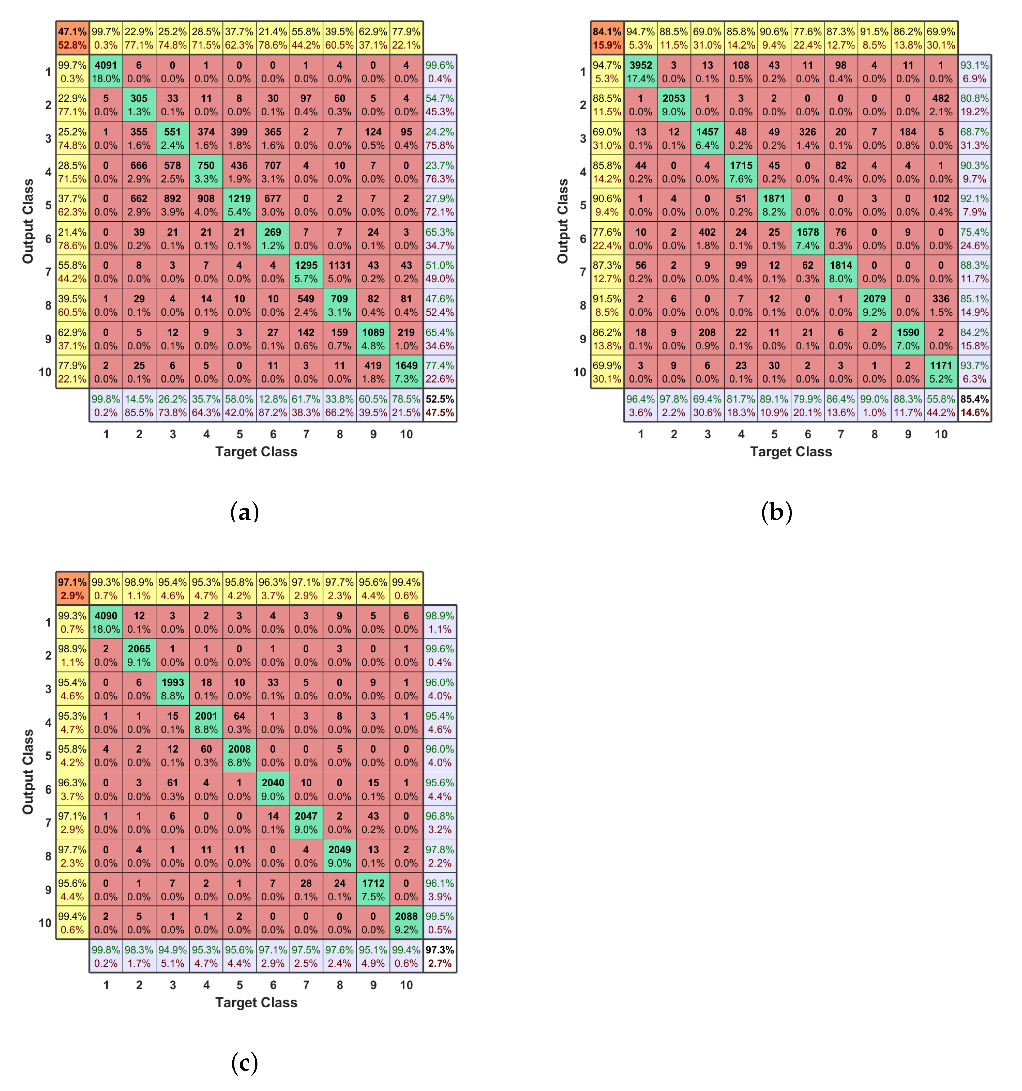
| Preprocessing steps 1,2,3,5 + DNN | 52.5% (low) | 85.4% (high) | 47.1% (low) | 84.1% (high) |
| Preprocessing steps 1–5 + DNN | 65.5% (low) | 90.6% (high) | 62.2% (low) | 89.7% (high) |
| Preprocessing steps 1–6 + DNN | 97.3% | 97.1% | ||
| Preprocessing steps 1–6 + MC-DNN | 98.1% | 97.9% | ||
| Preprocessing steps 1–6 + MC-DNN + Learning rate decay | 98.4% | 98.3% | ||
| Classification method in [22] | 46.8% | 43.0% | ||
| Classification method in [23] | 59.2% | 55.1% | ||
| Classification method in [24] | 87.4% | / | ||
Publisher’s Note: MDPI stays neutral with regard to jurisdictional claims in published maps and institutional affiliations. |
© 2021 by the authors. Licensee MDPI, Basel, Switzerland. This article is an open access article distributed under the terms and conditions of the Creative Commons Attribution (CC BY) license (https://creativecommons.org/licenses/by/4.0/).
Share and Cite
Yang, S.; Luo, Y.; Miao, W.; Ge, C.; Sun, W.; Luo, C. RF Signal-Based UAV Detection and Mode Classification: A Joint Feature Engineering Generator and Multi-Channel Deep Neural Network Approach. Entropy 2021, 23, 1678. https://doi.org/10.3390/e23121678
Yang S, Luo Y, Miao W, Ge C, Sun W, Luo C. RF Signal-Based UAV Detection and Mode Classification: A Joint Feature Engineering Generator and Multi-Channel Deep Neural Network Approach. Entropy. 2021; 23(12):1678. https://doi.org/10.3390/e23121678
Chicago/Turabian StyleYang, Shubo, Yang Luo, Wang Miao, Changhao Ge, Wenjian Sun, and Chunbo Luo. 2021. "RF Signal-Based UAV Detection and Mode Classification: A Joint Feature Engineering Generator and Multi-Channel Deep Neural Network Approach" Entropy 23, no. 12: 1678. https://doi.org/10.3390/e23121678
APA StyleYang, S., Luo, Y., Miao, W., Ge, C., Sun, W., & Luo, C. (2021). RF Signal-Based UAV Detection and Mode Classification: A Joint Feature Engineering Generator and Multi-Channel Deep Neural Network Approach. Entropy, 23(12), 1678. https://doi.org/10.3390/e23121678