Article

Bearing Fault Diagnosis Using Refined Composite Generalized Multiscale Dispersion Entropy-Based Skewness and Variance and Multiclass FCM-ANFIS

by
Mostafa Rostaghi
1,
Mohammad Mahdi Khatibi
1,*,
Mohammad Reza Ashory
1 and
Hamed Azami
2
1
Modal Analysis (MA) Research Laboratory, Faculty of Mechanical Engineering, Semnan University, Semnan 35131-19111, Iran
2
Department of Neurology and Massachusetts General Hospital, Harvard Medical School, Charlestown, MA 02129, USA
*
Author to whom correspondence should be addressed.
Entropy 2021, 23(11), 1510; https://doi.org/10.3390/e23111510
Submission received: 16 October 2021 / Revised: 7 November 2021 / Accepted: 8 November 2021 / Published: 14 November 2021
(This article belongs to the Special Issue Entropy in Data Analysis)

Abstract

:
Bearing vibration signals typically have nonlinear components due to their interaction and coupling effects, friction, damping, and nonlinear stiffness. Bearing faults affect the signal complexity at various scales. Hence, measuring signal complexity at different scales is helpful to diagnosis of bearing faults. Numerous studies have investigated multiscale algorithms; nevertheless, multiscale algorithms using the first moment lose important complexity data. Accordingly, generalized multiscale algorithms have been recently introduced. The present research examined the use of refined composite generalized multiscale dispersion entropy (RCGMDispEn) based on the second moment (variance) and third moment (skewness) along with refined composite multiscale dispersion entropy (RCMDispEn) in bearing fault diagnosis. Moreover, multiclass FCM-ANFIS, which is a combination of adaptive network-based fuzzy inference systems (ANFIS), was developed to improve the efficiency of rotating machinery fault classification. According to the results, it is recommended that generalized multiscale algorithms based on variance and skewness be examined for diagnosis, along with multiscale algorithms, and be used to achieve an improvement in the results. The simultaneous usage of the multiscale algorithm and generalized multiscale algorithms improved the results in all three real datasets used in this study.

1. Introduction

Bearings are among the most important and useful rotating machinery components [1]. A lack of timely diagnosis and replacement of bearings can disrupt the functionality of machinery. For instance, 40–50% of all electrical motor failures are associated with bearing failure [2]. Prompt fault detection in bearings can reduce financial loss and health risks.
The vibration signals of bearings usually exhibit a nonlinear behavior due to the effects of coupling and nonlinear interactions, friction, damping, and stiffness [3], and faults at different signal scales impact signal complexity. Hence, measurements of signal complexity at various scales can contribute to diagnosis and, thus, are commonly used.
Entropy is a measure of the disorder and predictability of the signal. It is one of the most powerful concepts used to evaluate signal characteristics [4]. Several entropies have been introduced to date, such as sample entropy (SampEn) and permutation entropy (PerEn). We recently introduced dispersion entropy (DispEn) [5] and demonstrated its advantage over PerEn and SampEn [5]. In addition to being fast, DispEn can provide a better representation of dynamic signal changes. PerEn considers only the order of the amplitudes with respect to each other, but DispEn takes into account the values of the amplitudes. Unlike SampEn, DispEn is also defined in short series [6]. Moreover, DispEn is relatively insensitive to noise [3]. Rostaghi et al. investigated the potential applications of DispEn in rotating machinery diagnosis and demonstrated its superiority over PerEn and approximate entropy (ApEn) [3]. Liu et al. combined DispEn and wavelet packets to extract the features used for bearing diagnosis [7]. They calculated the DispEn of each wavelet packet. Li et al. computed the intrinsic mode function (IMF) components of the signals via an improved complete ensemble empirical mode decomposition and used DispEn of the first few IMF components for bearing diagnosis [8]. Zhenzhen et al. employed variational mode decomposition (VMD) and DispEn for bearing diagnosis [9].
Disorder and complexity have different physical meanings [10,11]. Accordingly, conventional entropies cannot represent complexity without using other algorithms. Therefore, Costa et al. introduced the multiscale algorithm in 2002 to show complexity and analyze non-stationary and nonlinear signals [12]. They utilized this algorithm for SampEn. Subsequently, this algorithm was used for various entropies and enhanced multiple times. Aziz et al. introduced multiscale permutation entropy (MPerEn) [13]. Wu et al. introduced refined composite multiscale entropy (RCMSampEn) [14], Humeau-Heurtier et al. refined composite multiscale permutation entropy (RCMPerEn) [15], and Azami et al. refined composite multiscale dispersion entropy (RCMDispEn) [16].
Wang et al. utilized MDE for feature extraction in bearing diagnosis [17]. Congzhi et al. calculated the RCMDispEn of vibration signals and classified them using the support vector machine (SVM) for bearing diagnosis [18]. Zhang et al. utilized RCMDispEn and an improved SVM based on the whale optimization algorithm for fault detection of rolling bearings [19]. Lou et al. employed the RCMDispEn and the deep belief network-extreme learning machine optimized by the improved firework algorithm for rolling bearing sub-health recognition [20].
Various techniques have been used along with RCMDispEn for bearing diagnosis. These techniques include the fast ensemble empirical mode decomposition [21], adaptive sparest narrow-band decomposition [22], improved empirical wavelet transform [23,24], VMD [25], and improved VMD (IVMD) [26].
Costa et al. introduced generalized multiscale entropy (GMSE) in 2015 [27]. Generalized algorithms use other statistical properties, such as variance, for coarse-graining. Costa et al. specifically proposed and utilized the standard deviation (SD) and variance [27]. Wei et al. stated that, unlike the first moment, the second moment simultaneously separates the high and low frequency contents during coarse-graining [28], and employed variance-based generalized multiscale fuzzy entropy for diagnosis in rotating machinery [28]. Zheng et al. utilized generalized composite multiscale permutation entropy-based variance and the Laplacian score for bearing diagnosis [29]. Liu et al. detected bearing faults using generalized composite multiscale amplitude-aware permutation entropy-based variance and dual-tree complex wavelet packet transform [30].
Because of the advantages of DispEn-based algorithms over the SampEn-, FuzEn-, and PerEn-based algorithms [6], the present paper investigates refined composite generalized multiscale dispersion entropy (RCGMDispEn) based on variance and skewness with RCMDispEn for bearing fault diagnosis. It is worth mentioning that generalized multiscale dispersion entropy is proposed in this study for the first time to probe the properties of time series related to higher moments (the second and third moments, i.e., variance and skewness).
A combination of several classifiers was used to overcome the limitations of each classifier and achieve higher efficiency [31,32,33]. In numerous studies, several classifiers have been used with a classifier utilizing the results of the other classifiers for final classification [32,34,35]. Belaout et al. combined several Sugeno ANFIS to construct an output vector and introduced a multiclass ANFIS based on the winner-takes-all rule [36]. Similarly, multiclass FCM-ANFIS was used in this study to classify different kinds of faults.
The rest of the paper is organized as follows. Section 2.1 reviews the theory of DispEn, and Section 2.2 and Section 2.3 introduce the calculation of GMDispEn and RCGMDispEn, respectively. Section 3 introduces the theory behind combining ANFIS networks. In Section 4, RGMDispEn and GMDispEn methods are compared to MDispEn and RCMDispEn, respectively, in terms of diagnosis capability in simulated bearing signals. Section 5 uses three different datasets to demonstrate that simultaneously using RCGMDispEn and RCMDispEn in practical applications can provide better efficiency than MDispEn and RCMDispEn. Finally, Section 6 concludes the paper.

2. Generalized Refined Composite Multi-Scale Dispersion Entropy

2.1. Dispersion Entropy

The DispEn for the time series x = { x 1 ,   x 2 ,   x 3 , , x N } with a length of N can be calculated in six steps [5]:
Step 1. The signal is normalized between 0 and 1. The series y = { y 1 , y 2 , , y N } is obtained according to (1) from the normal cumulative distribution function (NCDF) of the series x :
y i = 1 σ 2 π x i e ( t γ ) 2 2 σ 2 d t
Here, σ and γ denote the SD and mean value of the time series x , respectively.
Step 2. Each member of the time series y is mapped to an integer between 1 and c (Equation (2)):
z i c = round ( c . y i + 0.5 )
c is the class parameter and indicates the number of classes that can be members of the time series z c . z i c is the ith member of the classified series z c .
Step 3. All the template vectors z j m , c ( j = 1 , 2 , , N ( m 1 ) d ) are created as follows:
z j m , c = { z j c , z j + d c , , z j + ( m 1 ) d c }
where m and d, respectively, denote the embedding dimension and time delay. The embedding dimension is the dimension of the state space used for reconstruction.
Step 4. Each series z j m , c is mapped to a pattern π v 0 v 1 v m 1 based on its values, while the following holds:
z j c = v 0 , z j + ( 1 ) d c = v 1 , z j + ( 2 ) d c = v 2 , , z j + ( m 1 ) d c = v m 1
The number of possible dispersion patterns that can be attributed to each series z j m , c is equal to c m , because each z j m , c has m members, and each of them can be an integer from 1 to c [5].
Step 5. For every c m dispersion patterns π v 0 v 1 v m 1 , the relative frequency is obtained using Equation (5); i.e., the number of dispersion patterns π v 0 v 1 v m 1 that are attributed to the series z j m , c is divided by the total number of m-dimensional series created.
p ( π v 0 v 1 v m 1 ) = N u m b e r { t | t N ( m 1 ) d , z j m , c has   type   π v 0 v 1 v m 1 } N ( m 1 ) d
p ( π v 0 v 1 v m 1 ) is the probability of dispersion pattern π v 0 v 1 v m 1 .
Step 6. DispEn with the embedding dimension m and number of classes c is calculated according to Equation (6):
D i s p E n ( x , m , c , d ) = p ( π v 0 v 1 v m 1 ) ln p ( π v 0 v 1 v m 1 )
To calculate the normalized DispEn (NDispEn) according to Equation (7), DispEn is divided by the largest possible DispEn.
N D i s p E n ( x , m , c , d ) = D i s p E n ( x , m , c , d ) ln ( c m )
When m or c is too large, the computation time is high, although it makes the DispEn values more reliable [5]. In addition, if the embedding dimension m is too small, the dynamic changes may not be detected in the signal, whereas large m may cause DispEn to be unable to observe small variations [5]. Based on the abovementioned facts and previous studies [3,5], the parameters m = 2 and c = 8 were used to calculate DispEn.

2.2. Generalized Multiscale Dispersion Entropy

Multiscale dispersion entropy (MDispEn) and generalized MDispEn (GMDispEn) compute DispEn in several consecutive scales based on the first and other momenta. The nth-moment-based generalized MDispEns are displayed as GMDispEnn. They are implemented as follows:
The signal is coarse-grained up to where the time series y n , ( τ ) , which is the time series x with the scale τ and the nth moment, is constructed [19]:
For MDispEn, based on the first moment:
y j 1 , ( τ ) = 1 τ i = ( j 1 ) τ + 1 j τ x i ,   1 j N τ
For GMDispEn2, based on the second moment (variance):
y j 2 , ( τ ) = 1 τ i = ( j 1 ) τ + 1 j τ   ( x i x ¯ j ) 2 ,   1 j N τ
For GMDispEn3, based on the third moment (skewness):
y j 3 , ( τ ) = 1 τ i = ( j 1 ) τ + 1 j τ   ( x i x ¯ j ) 3 ,   1 j N τ
where x ¯ j = 1 τ i = ( j 1 ) τ + 1 j τ x i .
The DispEn of the signal y n , ( τ ) is computed. Here, the mean and the SD of the main signal are used for mapping based on the NCDF before coarse-graining. This approach is similar to keeping r constant while calculating the multiscale entropy (MSE) such that r = 0.15 × D (original signal) for all scales.
With a change in τ , often carried out by adding 1 to τ , Steps 1 and 2 are repeated until the desired scale is reached.
For DispEn, the parameters must be set in such a way that the number of possible dispersion patterns becomes smaller than the signal length ( c m < L ) . Because the signal length for GMDispEn is reduced to L τ max due to coarse-graining, c m < L τ max is recommended for GMDispEn.

2.3. Generalized Refined Composite Multi-Scale Dispersion Entropy

In the calculation of the RCMDispEn and the nth-moment-based RCGMDispEn (RCGMDispEnn) with a scale factor of τ , τ different time series are constructed by coarse-graining based on the first and higher momenta in order and with different starting points. The relative frequency of the dispersion patterns is calculated from every τ time series. The kth coarse-grained time series x k n , ( τ ) = { x k , 1 n , ( τ ) , x k , 2 n , ( τ ) , } from the series x is obtained based on the nth moment and the scale τ as follows:
x k , j 1 , ( τ ) = 1 τ i = k + τ ( j 1 ) k + τ j 1 x i , 1 j N τ ,   1 k τ
x k , j 2 , ( τ ) = 1 τ i = k + τ ( j 1 ) k + τ j 1 ( x i x ¯ k , j ) 2 , 1 j N τ ,   1 k τ
x k , j 3 , ( τ ) = 1 τ i = k + τ ( j 1 ) k + τ j 1 ( x i x ¯ k , j ) 3 , 1 j N τ ,   1 k τ
where x ¯ k , j = 1 τ i = ( j 1 ) τ + k j τ + k 1 x i .
Hence, for every scale factor, RCGMDispEnn is defined as follows:
R C G M D i s p E n n ( x , m , c , d , τ ) = p ¯ ( π v 0 v 1 .... v m 1 ) . ln ( p ¯ ( π v 0 v 1 .... v m 1 ) )
where p ¯ ( π v 0 v 1 .... v m 1 ) = 1 τ k = 1 τ p k ( τ ) ( π v 0 v 1 .... v m 1 ) . p k ( τ ) ( π v 0 v 1 .... v m 1 ) is the relative frequency of the dispersion pattern π v 0 v 1 .... v m 1 in the time series x k n , ( τ ) .
In RCGMDispEn, τ coarse-grained time series with a length of L τ max are considered. Thus, the total number of samples calculated in RCGMDispEn is τ × L τ max L . Therefore, RCGMDispEn with a length of c m < L produces reliable results. This special property is significant in short-length signals.
It must be noted that the scale starts from 2 for calculating GMDispE2 and RCGMDispE2, and from 3 for calculating GMDispE3 and RCGMDispE3 [37,38].

3. Multiclass Adaptive Neuro-Fuzzy Classifier

3.1. Adaptive Neuro-Fuzzy Inference System (ANFIS)

ANFIS is a fuzzy model expressed in the form of a neural network [39]. It is characterized by a synergic collaboration between the fuzzy theory and neural networks. ANFIS combines a treatment of the uncertainty and interpretability of fuzzy systems with the learning capability of neural networks [40,41]. It utilizes neural network learning algorithms to estimate the parameters of the fuzzy model [42].
An ANFIS structure is composed of five layers with nodes in the same layer possessing the same function family, as explained below:
First layer: In this layer, the membership degrees of each input with respect to the membership functions are calculated. Various membership functions can be employed here. Because the partial derivatives of the Gaussian function parameters are smooth, the Gaussian function was used in this research:
μ i j ( x s j ) = exp ( ( x s j c i j ) 2 2 σ i j 2 )
Here, μ i j represents the membership of the Gaussian function with respect to the ith rule and jth feature, and x s j denotes the jth feature of the sth sample. The parameters c i j and σ i j respectively represent the center and width of the Gaussian function.
Second layer: In this layer, the fuzzy implication in each node is computed using the input membership degrees. θ i c , which is the implication of the ith rule for the sample x c , is obtained as follows:
θ i c = j = 1 N μ i j ( x c j )
Here, N denotes the number of input features x c .
Third layer: In this layer, the ratio of the implication of the rule associated with every node to the total rule implications is computed in every node. The normalized implication of the ith node ( θ i c ¯ ) is determined as follows:
θ i c ¯ = θ i c i = 1 M θ i c
M equals the number of rules.
Fourth layer: The nodes in this layer are adaptive nodes. The weighted output of each node in this layer φ i c is obtained by multiplying θ i c ¯ with a corresponding first-degree polynomial ( f i c ):
φ i c = θ i c . ¯ f i c
The coefficients of the polynomial f i c and the coefficients c i j and σ i j corresponding to the first layer are updated by the learning algorithms of the neural network.
Fifth layer: This layer contains a single fixed node that calculates the output f o u t :
f o u t ( x c ) = i = 1 M φ i c = i = 1 M θ i c ¯ . f i c
In this paper, fewer fuzzy rules were obtained by using fuzzy c-means (FCM), which automatically constructs a fuzzy rule base for ANFIS. A combination of the least-squares method and the backpropagation gradient descent method was used to adjust the membership functions and other parameters.

3.2. Fuzzy C-Means

FCM is a clustering algorithm that assigns each data point to a cluster with a specific degree of membership. Dunn introduced this algorithm [43] and Bezdek subsequently improved it [44,45].
FCM employs the minimization of the objective function [45]:
J m ( u , c ) = j = 1 D i = 1 N μ i j m x i c j 2
where N and D represent the number of data points and clusters, respectively. Moreover, x i denotes the ith data point, and c j is the center of the jth cluster. μ i j is the membership degree of x i with respect to the jth cluster, and m represents the fuzziness parameter. . denotes the Euclidean distance.
The objective function is minimized via an iterative process of updating the fuzzy membership degrees and the cluster centers [46]. The steps to implementing FCM are as follows [45,47]:
1-The membership degrees of the clusters μ i j are randomly initialized.
2-The centers and membership degrees of the clusters are calculated as below:
c j = i = 1 D μ i j m x i i = 1 D μ i j m
3-The membership degrees of the clusters are updated as follows:
μ i j = 1 k = 1 N ( x i c j x i c k ) 2 m 1
4-The objective function J m is computed.
5-Steps 2 to 4 are repeated until a minimum threshold for the objective function or the maximum number of iterations is reached.

3.3. Multiclass FCM-ANFIS

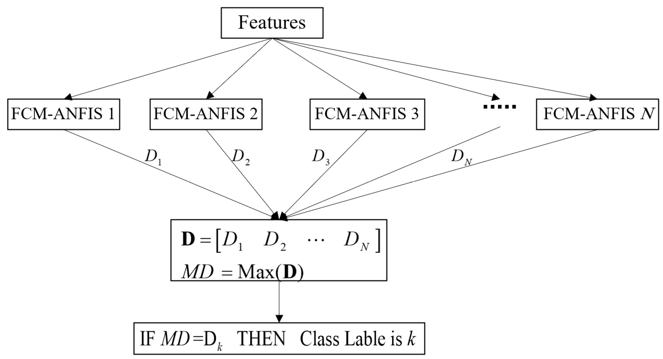
A combination of several classifiers is used to overcome the limitations of each classifier and achieve higher efficiency [34]. Each Sugeno ANFIS may be considered a binary classifier, and a set of them can be used in multiclass classification problems [36]. The final inference can take place via the winner-takes-all rule [36]. Accordingly, multiclass FCM-ANFIS was employed in this research. In this technique, every FCM-ANFIS examines the possibility of assigning a specific class to each input sample. Specifically, the kth FCM-ANFIS examined the possibility of assigning the class k to the inputs, and the target was considered to be 1 for the class k and zero for the rest of the classes. The final class is the one whose FCM-ANFIS has the largest output:
max ( [ o u t p u t ( FCM-ANFIS 1 ) , , o u t p u t ( FCM-ANFIS N ) ] ) = o u t p u t ( FCM-ANFIS k ) Final   output = Class   k
Figure 1 displays the implementation of multiclass FCM-ANFIS.

4. Analysis of a Simulated Bearing Signal

The vibration signal of ball bearing with an outer race fault was simulated as follows:
x ( t ) = x series   of   impulses + x harmonic   component + n ( t )
where x series   of   impulses and x harmonic   component represent the impulse series and the harmonic series, respectively, and n(t) denotes the noise.
Based on previous studies [48,49], x series   of   impulses was modeled using Equation (24):
x series   of   impulses = k = 1 m n = 1 n A e 2 ξ π f n ( t k f f i = 1 k τ k ) sin ( 2 π f n 1 ξ 2 ( t k f f i = 1 k τ k ) )
f n represents the resonance frequencies of the bearing, which are significantly higher than the fault frequency f f . τ k represents a small random change in the interval between two impulses. The ball slipping effect changes the period randomly to k f f τ k . Hence, for every k, τ k was considered to be a random number from a normal distribution with a zero mean and standard deviation of σ τ = 0.005 × 1 f f .
Two sinusoidal functions were employed for the harmonic part of Equation (23) [50,51]:
x harmonic   component = m = 1 2 B m sin ( 2 π m f r t )
In this simulation, the characteristic frequency of the fault and the damping factor were assumed to be f f = 100   Hz and ξ = 0.03 . Moreover, f 1 = 2   KHz , f 2 = 3.5   KHz represent the resonance frequencies of the bearing, and A = 1 denotes the magnitude of the impulse amplitude, which is a measure of the damage intensity. In addition, the rotor frequency was considered to be f r = 30   Hz , and B 1 = 0.2 and B 2 = 0.12 represent the amplitudes of the first and second harmonics of the rotor, respectively. The signal of a healthy bearing was modeled by eliminating the fault impulses.
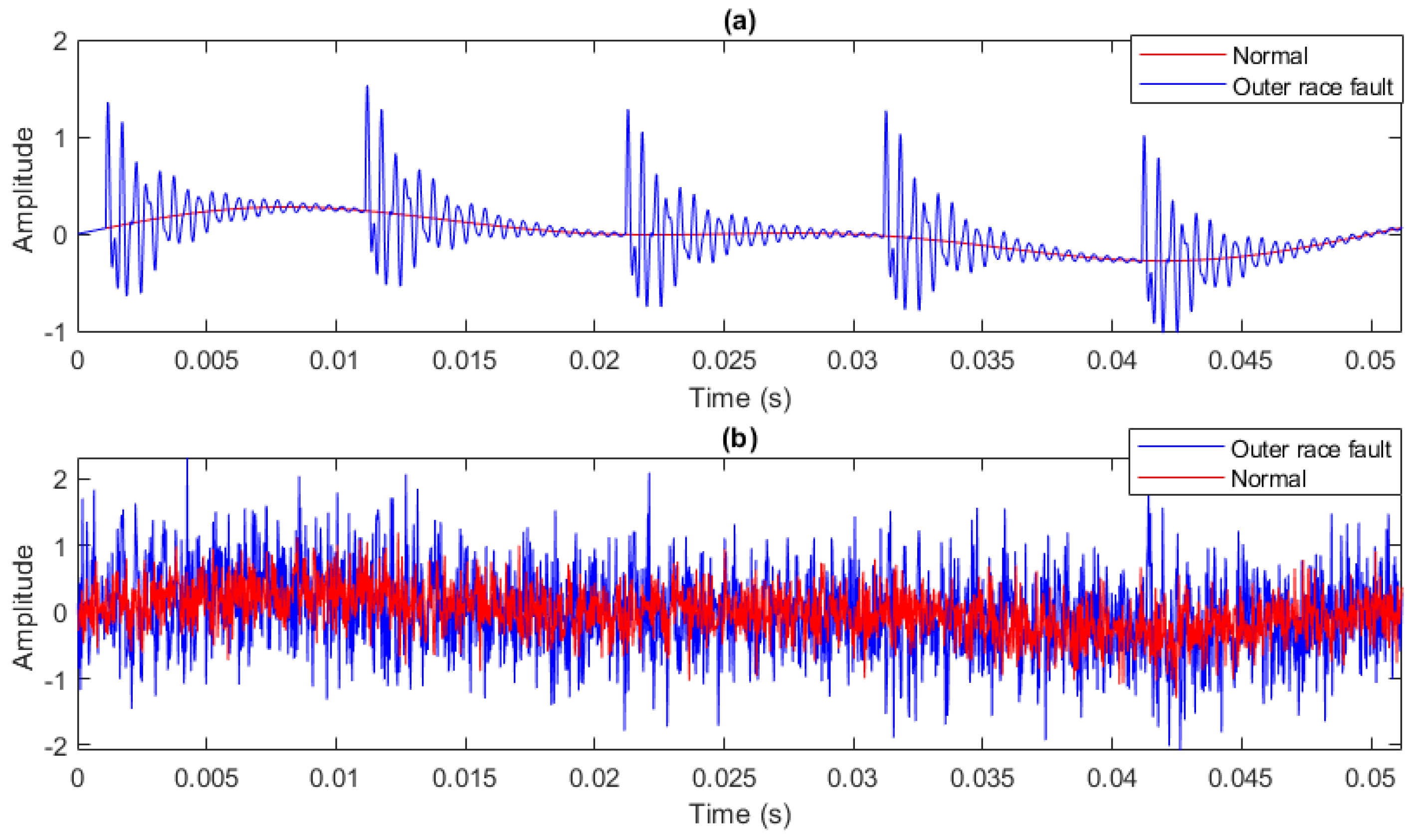
Fifty independent healthy and faulty bearing signals with a length of 2048 data points and a sampling frequency of 40 kHz were simulated. Moreover, Gaussian noise was added to them with the variance ratio of signal to noise of 0.257 [52]. Figure 2 shows an example of these signals.
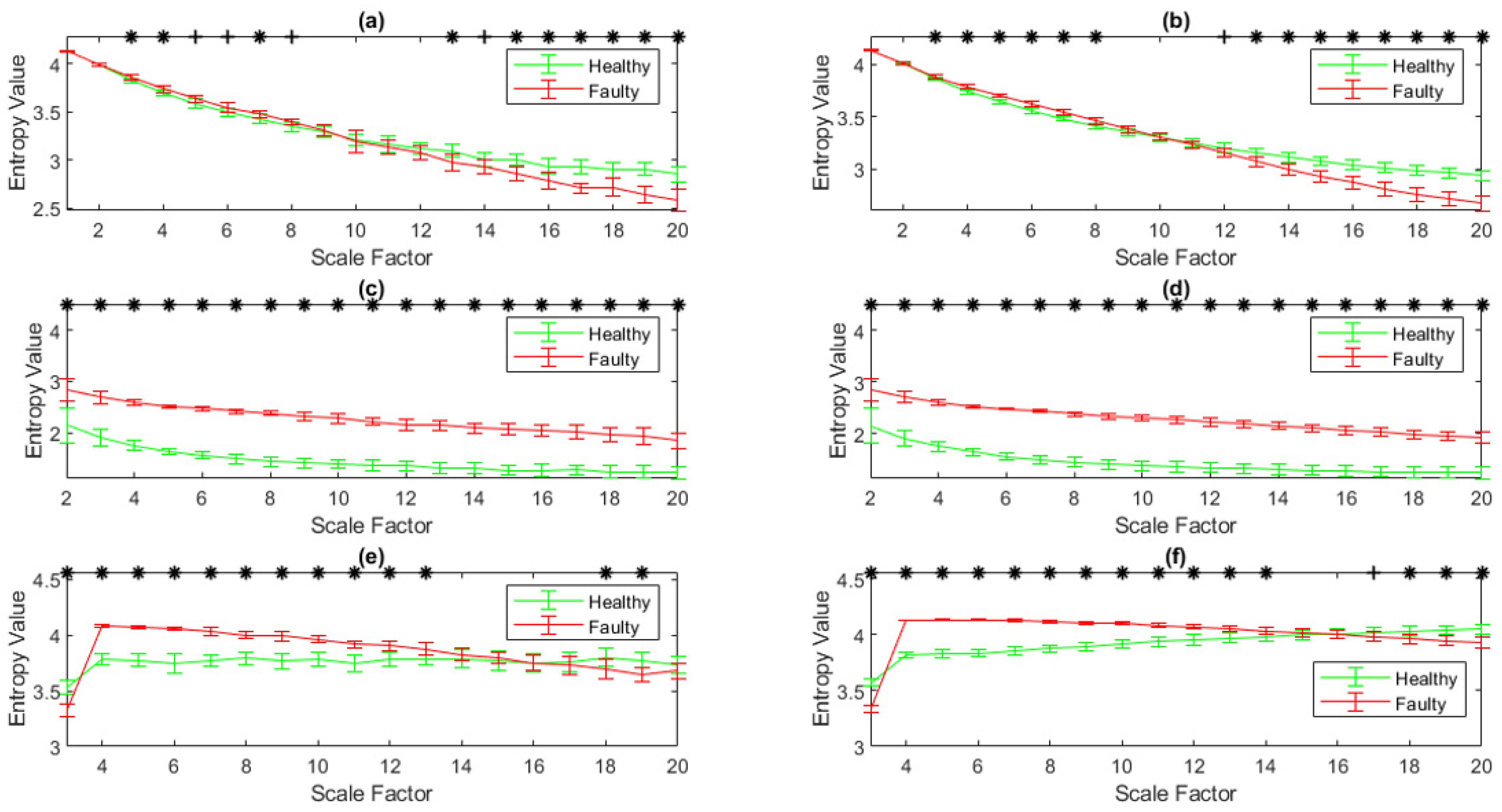
MDispEn, GMDispEn2, GMDispEn3, RCMDispEn, RCGMDispEn2, and RCGMDispEn3, were calculated for the simulated signals, with the results displayed in Figure 3. In this figure, p-values smaller than 0.05 are identified with asterisks. According to Figure 3, RCMDispEn, RCGMDispEn2, and RCGMDispEn3 possess higher fault distinguishing capability than MDispEn, GMDispEn2, and GMDispEn3, respectively, and their results have a smaller standard deviation. Distinguishing abilities of the bearing faults using the generalized methods are also displayed.
Hedges’ g effect size [53] was used to evaluate the capability of these methods in discriminating the faulty from healthy ball bearing signals. The results are shown in Table 1. As can be seen, the GMDispEn2, GMDispEn3, RCGMDispEn2, and RCGMDispEn3 algorithms effectively show the differences between the healthy and the faulty conditions, similar to MDispEn and RCMDispEn. RCMDispEn, RCGMDispEn2, and RCGMDispEn3 have larger size effects and better fault separation capability than MDispEn, GMDispEn2, and GMDispEn3, respectively.

5. Analysis of the Experiments

5.1. Analysis of the Vibration Signals Acquired from the Case Western Reserve University Dataset

This section uses datasets from Case Western Reserve University (CWRU), US [54], with a sampling frequency of 48 kHz. The experimental set-up includes a three-phase induction motor, a torque transducer, and a dynamometer. The ball-bearing vibration signals were collected using an accelerometer installed on the motor housing at the drive end of the motor.
The signals consisted of 10 different fault conditions: healthy, ball fault, inner race fault, and outer race fault with intensities of 0.021″, 0.007″, and 0.014″. The shaft rotating speeds were 1772, 1750, and 1730 rpm.
A detailed description of the data set is shown in Table 2. For each condition, 180 samples with a length of 2048 were separated from the dataset signals with no overlap between any two samples.
Specifically, 72, 18, and 90 signals were used for training, validation, and testing, respectively. MDispEn, GMDispEn2, GMDispEn3, RCMDispEn, RCGMDispEn2, and RCGMDispEn3 were calculated for all the signals, and their values were used in 20 scales as features for fault detection and classification. A binary vector was used as the target vector for every bearing condition. This binary vector had a length of 10 because 10 conditions were being studied. This research employed 10 FCM-ANFIS, each of which detected one element in the target vector.
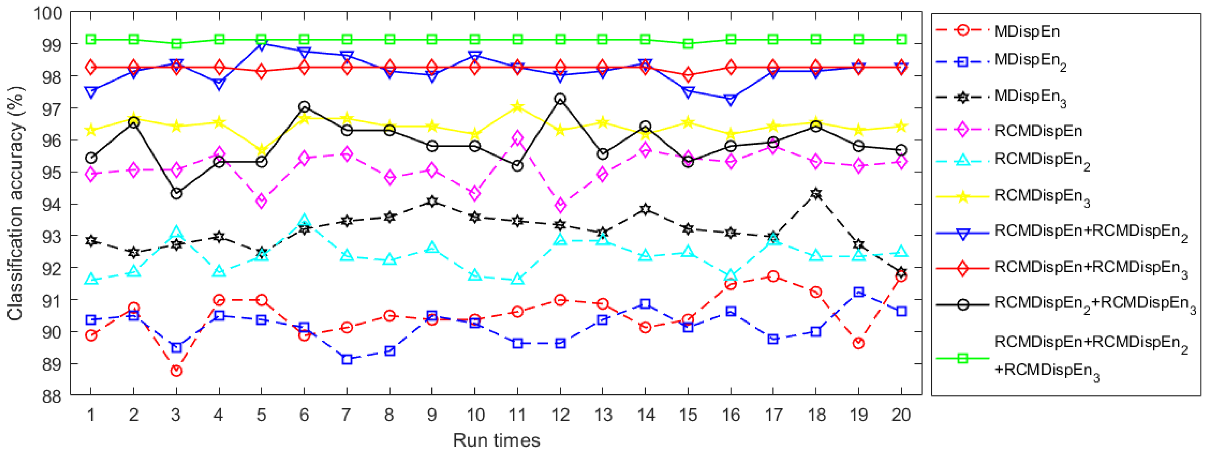
The faulty conditions classification using multiclass FCM-ANFIS was performed 20 times with different inputs. The results of classifying these features are displayed in Figure 4 and Table 3. In this example, RCMDispEn, RCGMDispEn2, and RCGMDispEn3 performed better at classification than MDispEn, GMDispEn2, and GMDispEn3, respectively. Moreover, the simultaneous use of RCMDispEn, RCGMDispEn2, and RCGMDispEn3 as the classifier inputs produced the most accurate classification. Table 4 represents the confusion matrix of the best performance using these inputs.

5.2. Analysis of the Signals Acquired from the PHMAP 2021 Data Challenge Dataset

Part of the PHMAP 2021 data challenge dataset [55] was used in this section. The studied equipment consists of an oil injection screw compressor, containing a 15 kW and 3600 rpm motor and a 7200 rpm screw axis. This paper used data acquired using an accelerometer installed on the motor with a sampling frequency of 10,544 samples per second.
Three fault conditions were examined: (1) high Looseness of V-belt, (2) faulty bearing, and (3) fault-free condition. Three hundred independent signal samples with a length of 1024 samples were separated for each fault condition.
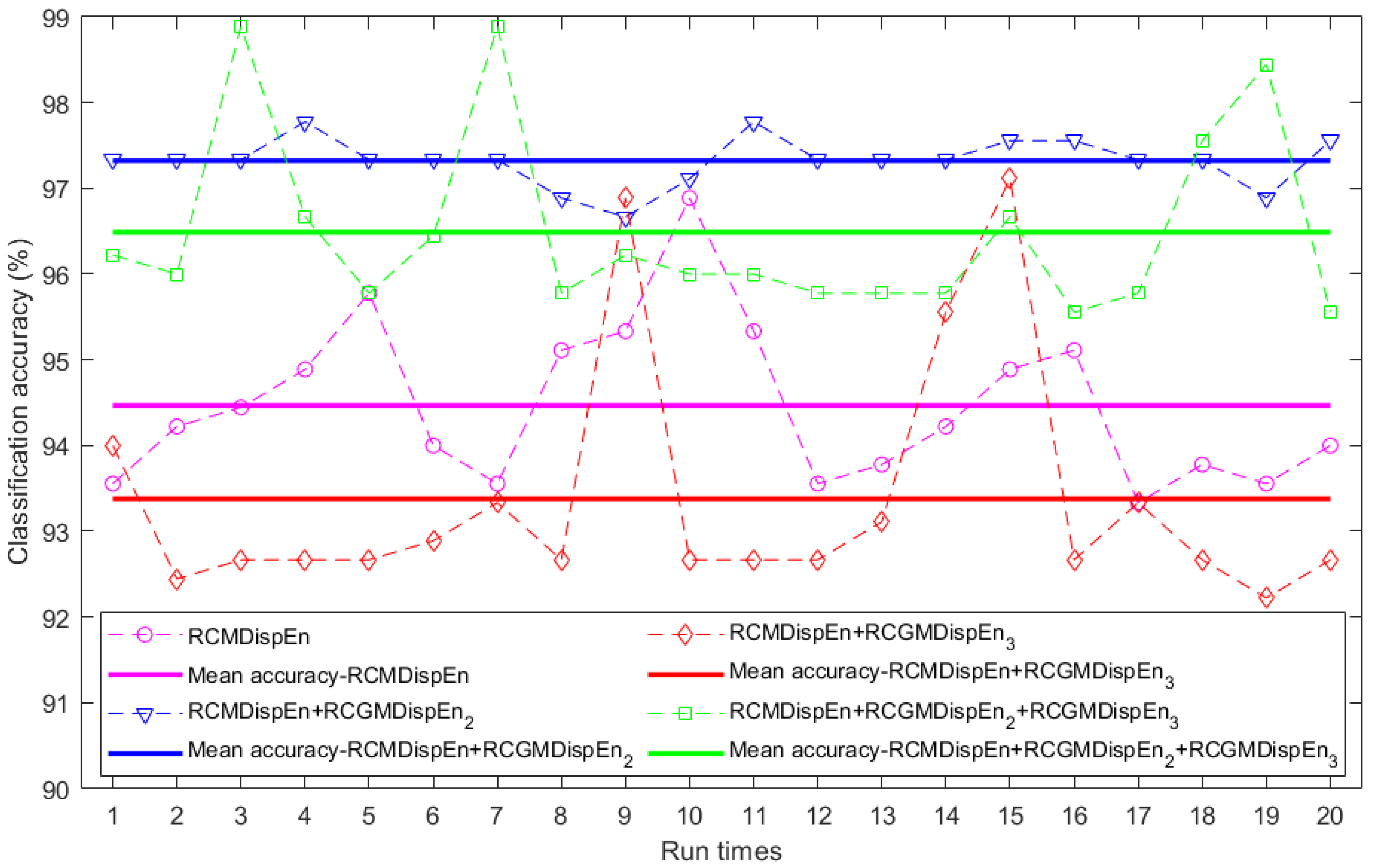
MDispEn, RCMDispEn, GMDispEn2, RCGMDispEn2, GMDispEn3, and RCGMDispEn3 were calculated for all the signals, and their values were used in 20 scales as features for fault detection and classification. For each condition, 120, 30, and 150 samples were used for training, validation, and testing, respectively. These data were classified 20 times using multiclass FCM-ANFIS. The results are displayed in Figure 5 and Table 5. As can be seen, the highest accuracy was achieved by the combined use of RCMDispEn, RCGMDispEn2, and RCGMDispEn3 as inputs. However, the mean accuracy of RCMDispEn and RCGMDispEn2 as simultaneous inputs was greater than that of other inputs. These results confirm the proposal of this paper regarding the use of generalized multiscale entropies with multiscale entropies to improve the results. The best classification results are displayed in Table 6.

5.3. Analysis of Vibration Signals Acquired from the Paderborn University Dataset

The data used in this section were from the ball bearing data collected in the Mechanical Engineering Construction and Drive Technology (KAt) Research data center, Paderborn University, Germany [56,57].
The classification of the datasets used in the present work is presented in Table 7, which represents three different fault conditions: (1) inner race damage, (2) outer race damage, and (3) healthy. The vibration signals corresponding to different bearing fault conditions under different operating conditions, shown in Table 8, were collected with a sampling frequency of 64,000 Hz.
A signal with a length of 1024 was separated from the beginning of every measured vibration signal, with 60 signals separated from each dataset, to obtain a total of 300 signals for each fault condition.
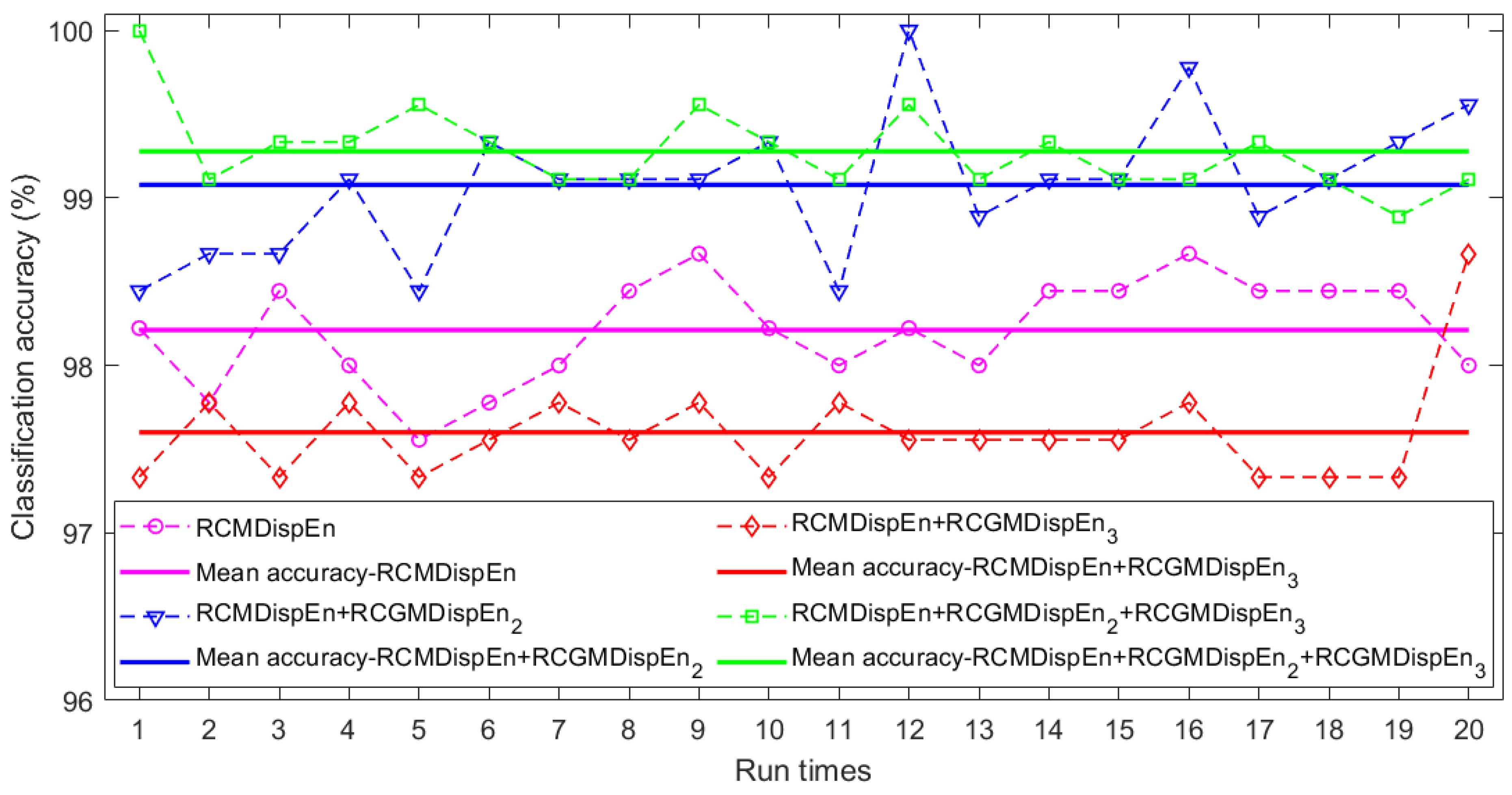
MDispEn, RCMDispEn, GMDispEn2, RCGMDispEn2, GMDispEn3, and RCGMDispEn3 were calculated for all the signals, and their values were used in 20 scales as features for fault detection and classification. For each condition, 120, 30, and 150 samples were used for training, validation, and testing, respectively. These data were classified 20 times using multiclass FCM-ANFIS. The results, displayed in Figure 6 and Table 9, confirm the suggestion made by the present study. Specifically, the highest classification accuracy corresponds to the features extracted by the combination of RCMDispEn, RCGMDispEn2, and RCGMDispEn3. Moreover, the smallest classification accuracy corresponds to the features extracted by RCMDispEn, RCGMDispEn2, and RCGMDispEn, separately.

6. Conclusions

The present paper investigated the simultaneous use of refined composite MDE based on different moments (i.e., first, second, and third moments, respectively, denote average, variance, and skewness respectively) to probe properties of the signals related to higher moments in bearing fault diagnosis. To this end, a bearing simulation example and three real datasets were utilized. Furthermore, the bearing fault classification was performed using multiclass FCM-ANFIS to examine the proposed technique. The results indicated that our developed RCGMDispEn3 and RCGMDispEn2 are more capable in separating bearing fault conditions compared to GMDispEn3 and GMDispEn2. Moreover, the combined use of RCGMDE, RCGMDE2, and RCGMDE3 produces better results than using one or two of these approaches in bearing fault diagnosis. The authors suggest investigating the potential of simultaneously using generalized multiscale and multiscale algorithms in other fields.

Author Contributions

Conceptualization, M.R. and H.A.; Investigation, H.A.; Methodology, M.R.; Project administration, M.R.A.; Supervision, M.M.K.; Writing—original draft, M.R.; Writing—review & editing, H.A. All authors have read and agreed to the published version of the manuscript.

Funding

This research received no external funding.

Institutional Review Board Statement

Not applicable.

Informed Consent Statement

Not applicable.

Data Availability Statement

The data that use in this study are openly available in CWRU datasets at https://engineering.case.edu/bearingdatacenter , PHMAP 2021 datasets at http://phmap.org/data-challenge , and KAt datasets at https://mb.uni-paderborn.de/kat/forschung/datacenter/bearing-datacenter/.

Conflicts of Interest

The authors declare no conflict of interest.

References

  1. Zhang, L.; Xiong, G.; Liu, H.; Zou, H.; Guo, W. Bearing fault diagnosis using multi-scale entropy and adaptive neuro-fuzzy inference. Expert Syst. Appl. 2010, 37, 6077–6085. [Google Scholar] [CrossRef]
  2. Nandi, S.; Toliyat, H.A.; Li, X. Condition Monitoring and Fault Diagnosis of Electrical Motors—A Review. IEEE Trans. Energy Convers. 2005, 20, 719–729. [Google Scholar] [CrossRef]
  3. Rostaghi, M.; Reza, M.; Azami, H. Application of dispersion entropy to status characterization of rotary machines. J. Sound Vib. 2019, 438, 291–308. [Google Scholar] [CrossRef]
  4. Azami, H.; Escudero, J. Improved multiscale permutation entropy for biomedical signal analysis: Interpretation and application to electroencephalogram recordings. Biomed. Signal Process. Control 2016, 23, 28–41. [Google Scholar] [CrossRef] [Green Version]
  5. Rostaghi, M.; Azami, H. Dispersion Entropy: A Measure for Time-Series Analysis. IEEE Signal Process. Lett. 2016, 23, 610–614. [Google Scholar] [CrossRef]
  6. Azami, H.; Escudero, J. Amplitude- and Fluctuation-Based Dispersion Entropy. Entropy 2018, 3, 210. [Google Scholar] [CrossRef] [Green Version]
  7. Liu, W.; Shen, J.; Yang, X. Rolling bearing fault detection approach based on improved dispersion entropy and AFSA optimized SVM. Int. J. Electr. Eng. Educ. 2020. [Google Scholar] [CrossRef]
  8. Li, R.; Ran, C.; Luo, J.; Feng, S. Rolling bearing fault diagnosis method based on dispersion entropy and SVM. In Proceedings of the 2019 International Conference on Sensing, Diagnostics, Prognostics, and Control (SDPC), Beijing, China, 15–17 August 2019; pp. 596–600. [Google Scholar]
  9. Jin, Z.; He, D.; Chen, Y.; Liu, C.; Shan, S. Research on Fault Diagnosis Method of Train Rolling Bearing Based on Variational Modal Decomposition and Bat Algorithm-Support Vector Machine. J. Phys. Conf. Ser. 2021, 1820, 12170. [Google Scholar] [CrossRef]
  10. Richman, J.S.; Moorman, J.R. Physiological time-series analysis using approximate entropy and sample entropy. Am. J. Physiol. Circ. Physiol. 2000, 278, H2039–H2049. [Google Scholar] [CrossRef] [Green Version]
  11. Yang, A.C.; Tsai, S. Progress in Neuro-Psychopharmacology & Biological Psychiatry Is mental illness complex? From behavior to brain. Prog. Neuropsychopharmacol. Biol. Psychiatry 2013, 45, 253–257. [Google Scholar]
  12. Costa, M.; Goldberger, A.L.; Peng, C.K. Multiscale Entropy Analysis of Complex Physiologic Time Series. Phys. Rev. Lett. 2002, 89, 6–9. [Google Scholar] [CrossRef] [PubMed] [Green Version]
  13. Aziz, W.; Arif, M. Multiscale permutation entropy of physiological time series. In Proceedings of the 2005 Pakistan Section Multitopic Conference INMIC, Karachi, Pakistan, 24–25 December 2005. [Google Scholar]
  14. Wu, S.; Wu, C.; Lin, S.; Lee, K.; Peng, C. Analysis of complex time series using refined composite multiscale entropy. Phys. Lett. A 2014, 378, 1369–1374. [Google Scholar] [CrossRef]
  15. Humeau-Heurtier, A.; Wu, C.W.; Wu, S.D. Refined Composite Multiscale Permutation Entropy to Overcome Multiscale Permutation Entropy Length Dependence. IEEE Signal Process. Lett. 2015, 22, 2364–2367. [Google Scholar] [CrossRef]
  16. Azami, H.; Member, S.; Rostaghi, M.; Ab, D. Refined Composite Multiscale Dispersion Entropy and its Application to Biomedical Signals. IEEE Trans. Biomed. Eng. 2017, 64, 2872–2879. [Google Scholar]
  17. Wang, Z.; Zheng, L.; Wang, J.; Du, W. Research on novel bearing fault diagnosis method based on improved krill herd algorithm and kernel extreme learning machine. Complexity 2019, 2019, 4031795. [Google Scholar] [CrossRef]
  18. LI, C.; ZHENG, J.; PAN, H.; LIU, Q. Fault diagnosis method of rolling bearings based on refined composite multiscale dispersion entropy and support vector machine. China Mech. Eng. 2019, 30, 1713. [Google Scholar]
  19. Zhang, X.; Zhao, J.; Teng, H.; Liu, G. A novel faults detection method for rolling bearing based on RCMDE and ISVM. J. Vibroen. 2019, 21, 2148–2158. [Google Scholar] [CrossRef]
  20. Luo, H.A.O.; He, C.; Zhou, J.; Zhang, L.I. Rolling Bearing Sub-Health Recognition via Extreme Learning Machine Based on Deep Belief Network Optimized by Improved Fireworks. IEEE Access 2021, 9, 42013–42026. [Google Scholar] [CrossRef]
  21. Zhang, W.; Zhou, J. A Comprehensive Fault Diagnosis Method for Rolling Bearings Based on Refined Composite Multiscale Dispersion Entropy and Fast Ensemble Empirical Mode Decomposition. Entropy 2019, 21, 680. [Google Scholar] [CrossRef] [Green Version]
  22. Luo, S.; Yang, W.; Luo, Y. Fault diagnosis of a rolling bearing based on adaptive sparest narrow-band decomposition and refined composite multiscale dispersion entropy. Entropy 2020, 22, 375. [Google Scholar] [CrossRef] [PubMed] [Green Version]
  23. Zheng, J.; Huang, S.; Pan, H.; Jiang, K. An improved empirical wavelet transform and refined composite multiscale dispersion entropy-based fault diagnosis method for rolling bearing. IEEE Access 2020, 8, 168732–168742. [Google Scholar] [CrossRef]
  24. Cai, J.; Yang, L.; Zeng, C.; Chen, Y. Integrated approach for ball mill load forecasting based on improved EWT, refined composite multi-scale dispersion entropy and fireworks algorithm optimized SVM. Adv. Mech. Eng. 2021, 13, 1687814021991264. [Google Scholar] [CrossRef]
  25. Lv, J.; Sun, W.; Wang, H.; Zhang, F. Coordinated Approach Fusing RCMDE and Sparrow Search Algorithm-Based SVM for Fault Diagnosis of Rolling Bearings. Sensors 2021, 21, 5297. [Google Scholar] [CrossRef] [PubMed]
  26. Zhang, Y.; Tong, S.; Cong, F.; Xu, J. Research of feature extraction method based on sparse reconstruction and multiscale dispersion entropy. Appl. Sci. 2018, 8, 888. [Google Scholar] [CrossRef] [Green Version]
  27. Costa, M.D.; Goldberger, A.L. Generalized multiscale entropy analysis: Application to quantifying the complex volatility of human heartbeat time series. Entropy 2015, 17, 1197–1203. [Google Scholar] [CrossRef]
  28. Wei, Y.; Li, Y.; Xu, M.; Huang, W. Intelligent fault diagnosis of rotating machinery using ICD and generalized composite multi-scale fuzzy entropy. IEEE Access 2018, 7, 38983–38995. [Google Scholar] [CrossRef]
  29. Zheng, J.; Pan, H.; Yang, S.; Cheng, J. Generalized composite multiscale permutation entropy and Laplacian score based rolling bearing fault diagnosis. Mech. Syst. Signal Process. 2018, 99, 229–243. [Google Scholar] [CrossRef]
  30. Liu, W.; Yang, X.; Jinxing, S. An Integrated Fault Identification Approach for Rolling Bearings Based on Dual-Tree Complex Wavelet Packet Transform and Generalized Composite Multiscale Amplitude-Aware Permutation Entropy. Shock Vib. 2020, 2020, 8851310. [Google Scholar] [CrossRef]
  31. Fumera, G.; Roli, F. A theoretical and experimental analysis of linear combiners for multiple classifier systems. IEEE Trans. Pattern Anal. Mach. Intell. 2005, 27, 942–956. [Google Scholar] [CrossRef]
  32. Lei, Y.; He, Z.; Zi, Y.; Hu, Q. Fault diagnosis of rotating machinery based on multiple ANFIS combination with GAs. Mech. Syst. Signal Process. 2007, 21, 2280–2294. [Google Scholar] [CrossRef]
  33. Kittler, J.; Hater, M.; Duin, R.P.W. Combining classifiers. Proc. Int. Conf. Pattern Recognit. 1996, 2, 897–901. [Google Scholar]
  34. Yin, X.C.; Liu, C.P.; Han, Z. Feature combination using boosting. Pattern Recognit. Lett. 2005, 26, 2195–2205. [Google Scholar] [CrossRef]
  35. Mashao, D.J.; Skosan, M. Combining classifier decisions for robust speaker identification. Pattern Recognit. 2006, 39, 147–155. [Google Scholar] [CrossRef]
  36. Belaout, A.; Krim, F.; Mellit, A.; Talbi, B.; Arabi, A. Multiclass adaptive neuro-fuzzy classifier and feature selection techniques for photovoltaic array fault detection and classification. Renew. Energy 2018, 127, 548–558. [Google Scholar] [CrossRef]
  37. Yin, Y.; Wang, X.; Li, Q.; Shang, P. Generalized multivariate multiscale sample entropy for detecting the complexity in complex systems. Phys. A Stat. Mech. Its Appl. 2020, 545, 123814. [Google Scholar] [CrossRef]
  38. Xu, M.; Shang, P. Analysis of financial time series using multiscale entropy based on skewness and kurtosis. Phys. A Stat. Mech. Its Appl. 2018, 490, 1543–1550. [Google Scholar] [CrossRef]
  39. Li, C.; De Oliveira, J.L.V.; Cerrada, M.; Cabrera, D.; Sanchez, R.V.; Zurita, G. A systematic review of fuzzy formalisms for bearing fault diagnosis. IEEE Trans. Fuzzy Syst. 2018, 27, 1362–1382. [Google Scholar] [CrossRef]
  40. Pedrycz, W. Neurocomputations in relational systems. IEEE Trans. Pattern Anal. Mach. Intell. 1991, 13, 289–297. [Google Scholar] [CrossRef]
  41. Vitor, P.; Souza, D.C. Fuzzy neural networks and neuro-fuzzy networks : A review the main techniques and applications used in the literature. Appl. Soft Comput. J. 2020, 92, 106275. [Google Scholar]
  42. Dogantekin, E.; Dogantekin, A.; Avci, D.; Avci, L. An intelligent diagnosis system for diabetes on Linear Discriminant Analysis and Adaptive Network Based Fuzzy Inference System: LDA-ANFIS. Digit. Signal Process. 2010, 20, 1248–1255. [Google Scholar] [CrossRef]
  43. Dunn, J.C. A fuzzy relative of the ISODATA process and its use in detecting compact well-separated clusters. J. Cybern. 1973, 3, 32–57. [Google Scholar] [CrossRef]
  44. Bezdek, J.C. Pattern Recognition with Fuzzy Objective Function Algorithms; Plenum Press: New York, NY, USA, 1981; ISBN 9781475704525. [Google Scholar]
  45. Bezdek, J.C.; Ehrlich, R.; Full, W. FCM: The fuzzy c-means clustering algorithm. Comput. Geosci. 1984, 10, 191–203. [Google Scholar] [CrossRef]
  46. Pham, T.D. Fuzzy Recurrence Plots and Networks with Applications in Biomedicine; Springer: Cham, Switzerland, 2020; ISBN 9783030375294. [Google Scholar]
  47. The MathWorks Inc. FCM. Available online: https://www.mathworks.com/help/fuzzy/fcm.html (accessed on 4 May 2021).
  48. Zhao, Z.; Qiao, B.; Wang, S.; Shen, Z.; Chen, X. A weighted multi-scale dictionary learning model and its applications on bearing fault diagnosis. J. Sound Vib. 2019, 446, 429–452. [Google Scholar] [CrossRef]
  49. Tian, X.; Xi, J.; Rehab, I.; Abdalla, G.M.; Gu, F.; Ball, A.D. A robust detector for rolling element bearing condition monitoring based on the modulation signal bispectrum and its performance evaluation against the Kurtogram. Mech. Syst. Signal Process. 2018, 100, 167–187. [Google Scholar] [CrossRef]
  50. Kim, S.; An, D.; Choi, J.-H. Diagnostics 101: A Tutorial for Fault Diagnostics of Rolling Element Bearing Using Envelope Analysis in MATLAB. Appl. Sci. 2020, 10, 7302. [Google Scholar] [CrossRef]
  51. Kedadouche, M.; Liu, Z.; Vu, V.-H. A new approach based on OMA-empirical wavelet transforms for bearing fault diagnosis. Measurement 2016, 90, 292–308. [Google Scholar] [CrossRef]
  52. A complex filter for vibration signal demodulation in bearing defect diagnosis. J. Sound Vib. 2004, 276, 105–119. [CrossRef]
  53. Rosenthal, R. Parametric measures of effect size. In The Handbook of Research Synthesis; Cooper, H., Hedges, L.V., Eds.; Sage: New York, NY, USA, 1994; pp. 231–244. [Google Scholar]
  54. Case Western Reserve University Bearing Data Center Website. Available online: https://engineering.case.edu/bearingdatacenter/ (accessed on 23 June 2020).
  55. Data Challenge at PHMAP 2021. Available online: http://phmap.org/data-challenge/ (accessed on 18 June 2021).
  56. Lessmeier, C.; Kimotho, J.K.; Zimmer, D.; Sextro, W. KAt-Data Center, Chair of Design and Drive Technology; Paderborn University: Paderborn, Germany, 2019. [Google Scholar]
  57. Lessmeier, C.; Kimotho, J.K.; Zimmer, D.; Sextro, W. Condition monitoring of bearing damage in electromechanical drive systems by using motor current signals of electric motors: A benchmark data set for data-driven classification. In Proceedings of the PHM Society European Conference, Bilbao, Spain, 5–8 July 2016; Volume 3. [Google Scholar]
Figure 1. Implementation of multiclass FCM-ANFIS.
Entropy 23 01510 g001
Figure 2. Simulated signals corresponding to the healthy and faulty bearings (a) without noise; (b) with noise.
Entropy 23 01510 g002
Figure 3. Comparison of 50 independent simulated signals corresponding to healthy and faulty bearings at 20 scales. (a) MDispEn; (b) RCMDispEn; (c) GMDispEn2; (d) RCGMDispEn2; (e) GMDispEn3; (f) RCGMDispEn3.
Entropy 23 01510 g003
Figure 4. Classification accuracies of ball bearing fault diagnosis using ten different methods from the CWRU dataset.
Entropy 23 01510 g004
Figure 5. Results of classifying fault conditions: (1) high looseness of V-belt, (2) faulty bearing, and (3) fault-free condition using multiclass FCM-ANFIS with different inputs.
Entropy 23 01510 g005
Figure 6. Results of classification of bearing fault signals using multiclass FCM-ANFIS with different inputs.
Entropy 23 01510 g006
Table 1. Hedges’ g effect size of MDispEn, RCMDispEn, GMDispEn2, RCGMDispEn2, GMDispEn3, and RCGMDispEn3 in 20 scales on 50 independent healthy and faulty bearing signals.
ScaleMethods
MDispEnRCMDispEnGMDispEn2RCGMDispEn2GMDispEn3RCGMDispEn3
10.64930.6493----
20.22350.49152.23642.2569--
31.12421.73455.01365.58783.21196.9364
41.11832.467410.893310.77497.987214.1039
51.02302.930216.640617.72006.634012.5567
61.08752.078715.787817.25614.629812.3608
70.93972.084211.013714.06675.92289.5684
81.08431.45311.865112.46764.31298.9234
90.27160.755910.411612.03553.82958.1357
100.08860.23869.030311.00073.40576.2796
110.39810.43738.752410.57852.76314.1878
120.67080.97147.453710.02662.04092.8769
131.45991.61877.37579.50241.88162.0764
140.98792.06746.87958.75880.53271.2610
151.95792.75606.72288.82630.31140.3482
161.73763.10146.32368.53320.05660.2229
173.29263.31366.14387.96830.36840.9012
181.93793.64724.99627.43631.19231.5027
193.25483.78644.49186.86641.85312.0079
202.71944.02284.26446.07400.72432.4493
Table 2. Description of bearing data set.
Bearing ConditionDefect Size
(mm)
Label of
Classification
Normal01
Rolling element Fault0.17782
Rolling element Fault0.35563
Rolling element Fault0.53344
Inner race Fault0.17785
Inner race Fault0.35566
Inner race Fault0.53347
Outer race Fault0.17788
Outer race Fault0.53349
Table 3. The classification results of ball bearing faults using ten different inputs from the CWRU dataset.
Accuracy (%)
FeaturesMinMeanMax
MDispEn88.765490.567991.7284
GMDispEn289.135890.172891.2346
GMDispEn391.851993.160594.3210
RCMDispEn93.950695.142096.0494
RCGMDispEn291.604992.345793.4568
RCGMDispEn395.679096.419897.0370
RCMDispEn+ RCGMDispEn297.284098.179099.0123
RCMDispEn+ RCGMDispEn398.024798.253198.2716
RCGMDispEn2+ RCGMDispEn394.321095.876597.2840
RCMDispEn+RCGMDispEn2+ RCGMDispEn399.012399.123599.1358
Table 4. Confusion matrix of the testing set of the multiclass FCM-ANFIS using RCMDispEn, RCMDispEn, and RCMDispEn as the input.
True Label
123456789Sensitivity
Predicted Label19000000000100
20900000000100
3008810000098.87
4000870200097.75
50000900000100
6000108800098.88
7000100900098.90
80000000900100
9002000009097.83
Precision10010097.7896.6710097.78100100100AC * = 99.13
* AC is the accuracy.
Table 5. Results of classifying fault conditions: (1) high looseness of V-belt, (2) faulty bearing, and (3) fault-free condition using multiclass FCM-ANFIS with different inputs.
Accuracy (%)
FeaturesMinMeanMax
RCMDispEn93.333394.466796.8889
RCMDispEn + RCGMDispEn296.666797.322297.7778
RCMDispEn + RCGMDispEn392.222293.377897.1111
RCMDispEn + RCGMDispEn2 + RCGMDispEn395.555696.488998.8889
Table 6. Most accurate classification of three fault conditions: (1) high looseness of V-belt, (2) faulty bearing, and (3) fault-free condition using RCMDispEn, RCMDispEn2, and RCMDispEn3 as inputs.
True Condition
Belt Looseness HighBearing FaultNormalSensitivity (%)
Predicted conditionBelt Looseness High14800100
Bearing fault0150398.04
Normal2014798.66
Precision (%)98.6710098AC * = 98.89
* AC is the accuracy.
Table 7. Operating conditions.
No.Rotational Speed [rpm]Load Torque [Nm]Radial Force [N]
115000.71000
215000.11000
315000.7400
Table 8. Datasets used for three different bearing fault conditions.
Type of Bearing
HealthyOuter Ring DamageInner Ring Damage
Bearing CodeKI04KA04K001
KI14KA15K002
KI16KA16K003
KI18KA22K004
KI21KA30K005
Table 9. Classification results of bearing fault conditions: (1) inner race damage, (2) outer race damage, and (3) healthy.
Accuracy (%)
FeaturesMinMeanMax
RCMDispEn97.555698.2111198.6667
RCGMDispEn290.666791.3444591.7778
RCGMDispEn386.666789.6222292.2222
RCMDispEn + RCGMDispEn298.444499.07778100
RCMDispEn + RCGMDispEn397.333397.600098.6667
RCMDispEn + RCGMDispEn2 + RCGMDispEn398.888999.27778100
Publisher’s Note: MDPI stays neutral with regard to jurisdictional claims in published maps and institutional affiliations.