A Veritable Zoology of Successive Phase Transitions in the Asymmetric q-Voter Model on Multiplex Networks


Abstract
1. Introduction
2. -Voter Model on Single- and Multilayer Networks
2.1. The q-Voter Model on a Single Monoplex Clique
2.2. The q-Voter Model on a Monoplex Network
2.3. The Symmetric q-Voter Model on a Duplex Clique
2.4. Asymmetric q-Voter Model on Duplex Networks
3. Results
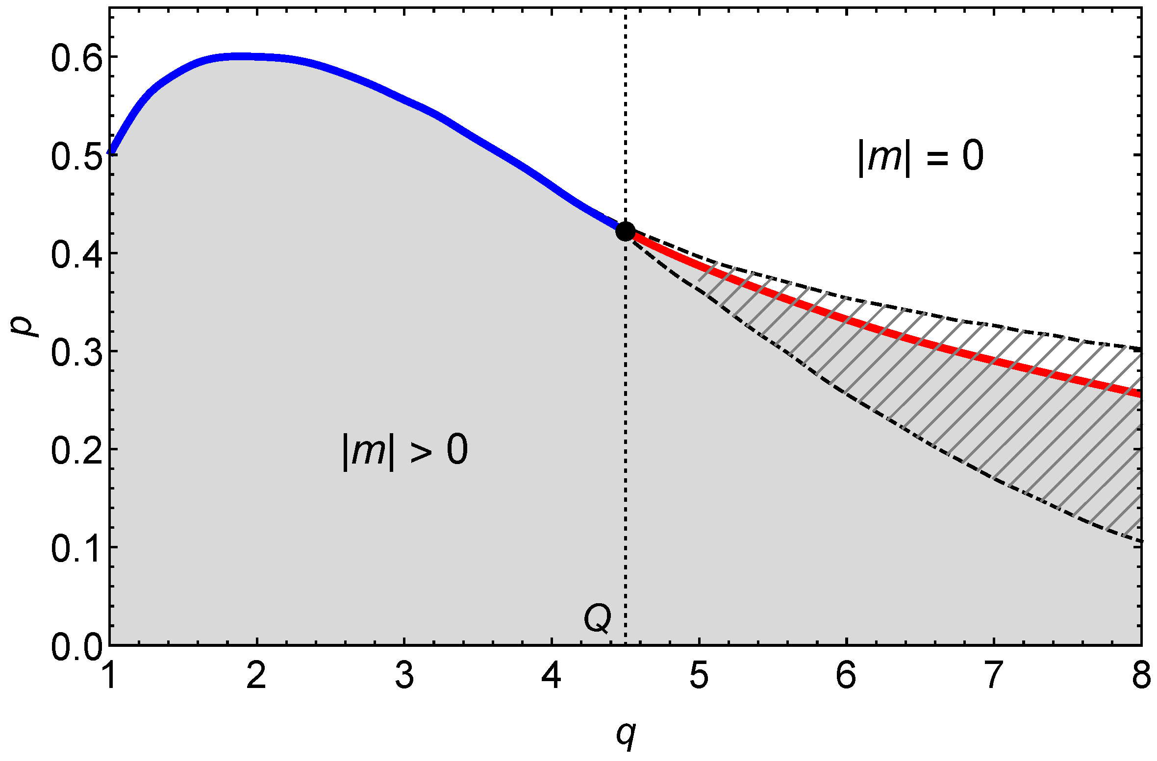
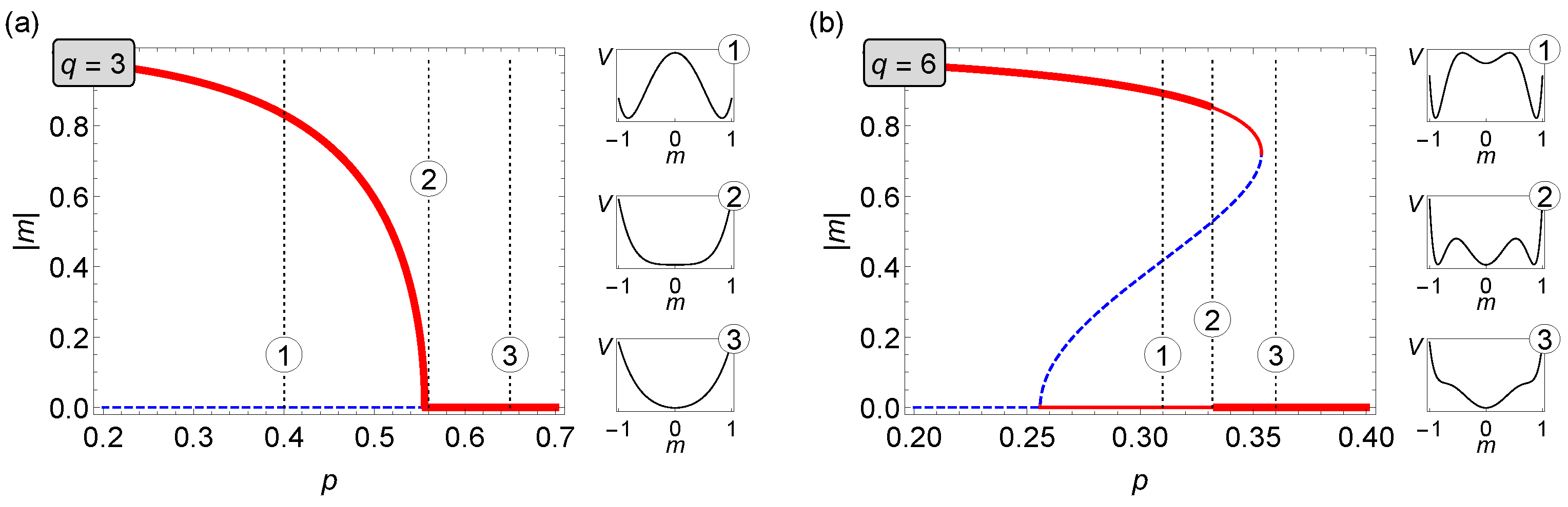
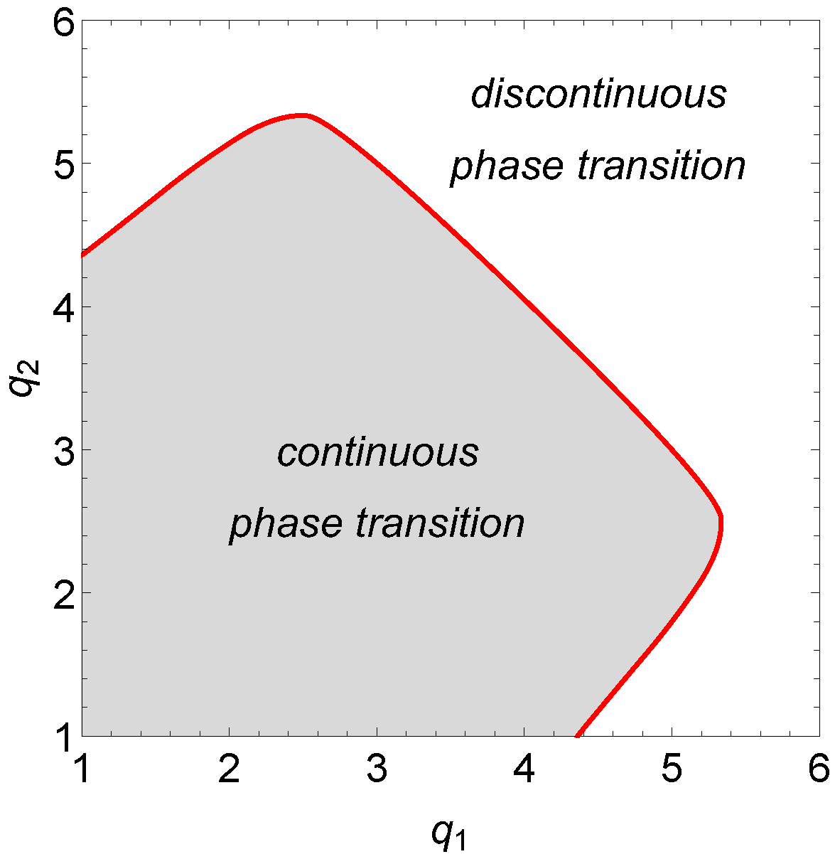
3.1. Symmetric q-Voter Model on Duplex Networks
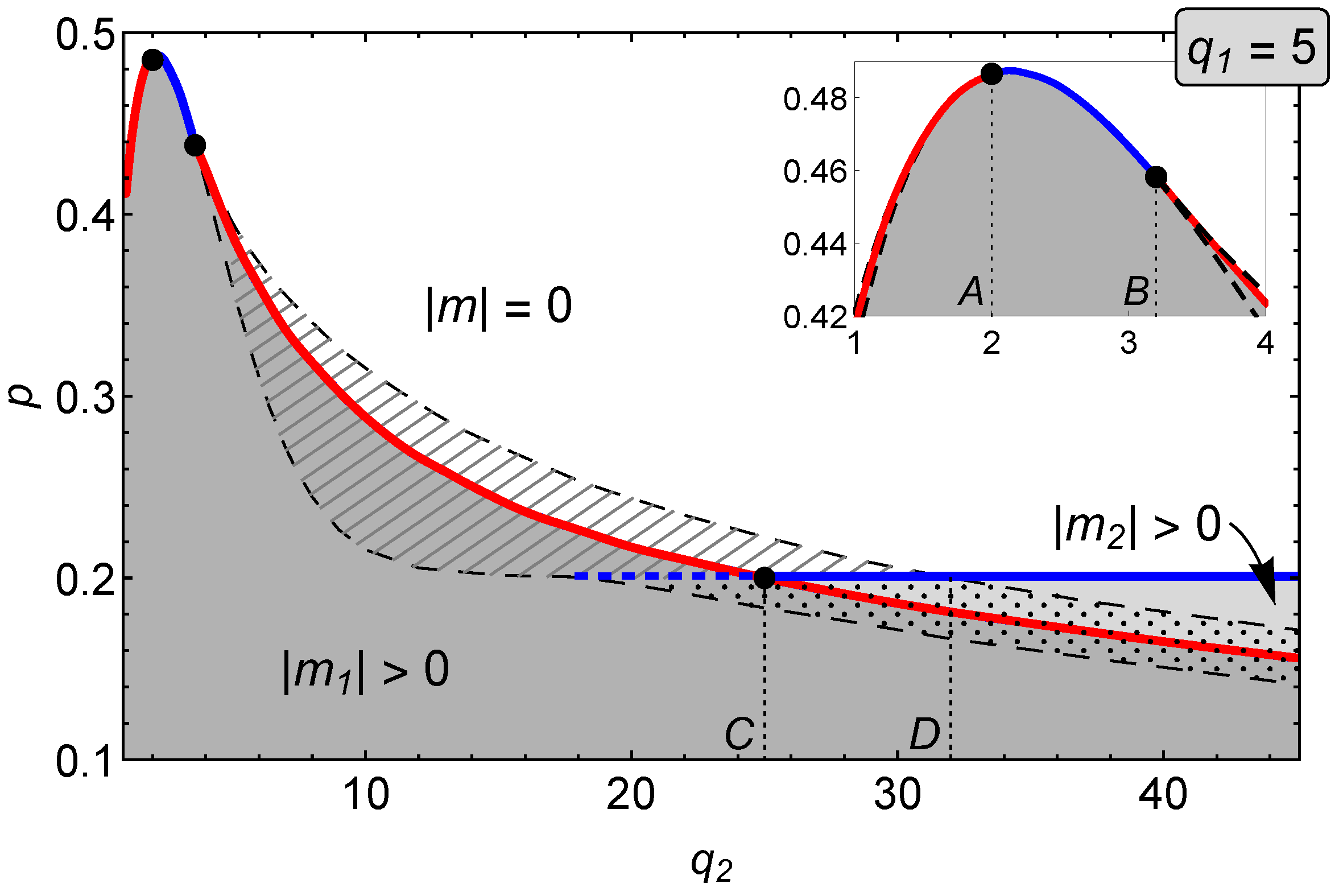
3.2. Asymmetric q-Voter Model on Duplex Networks
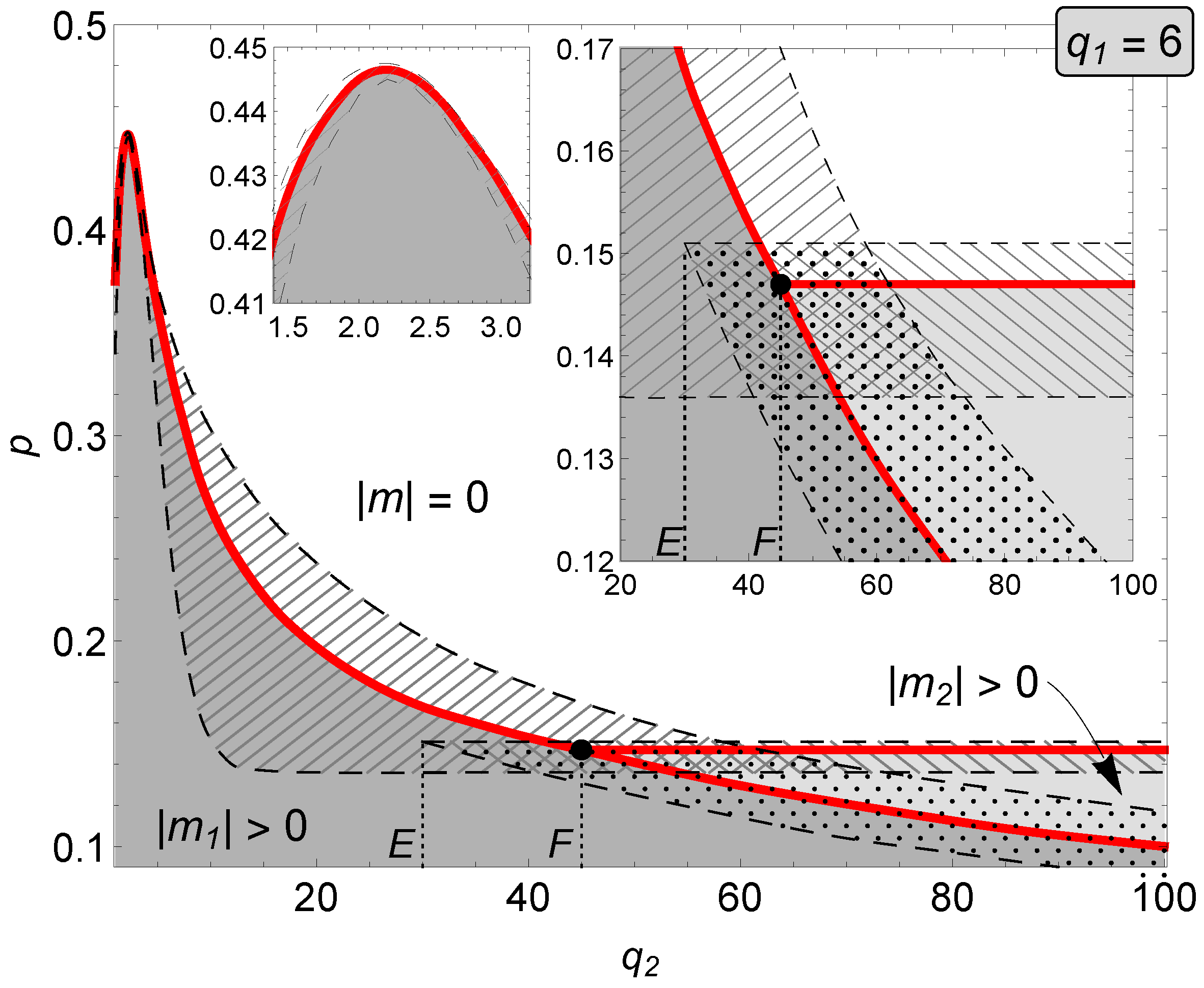
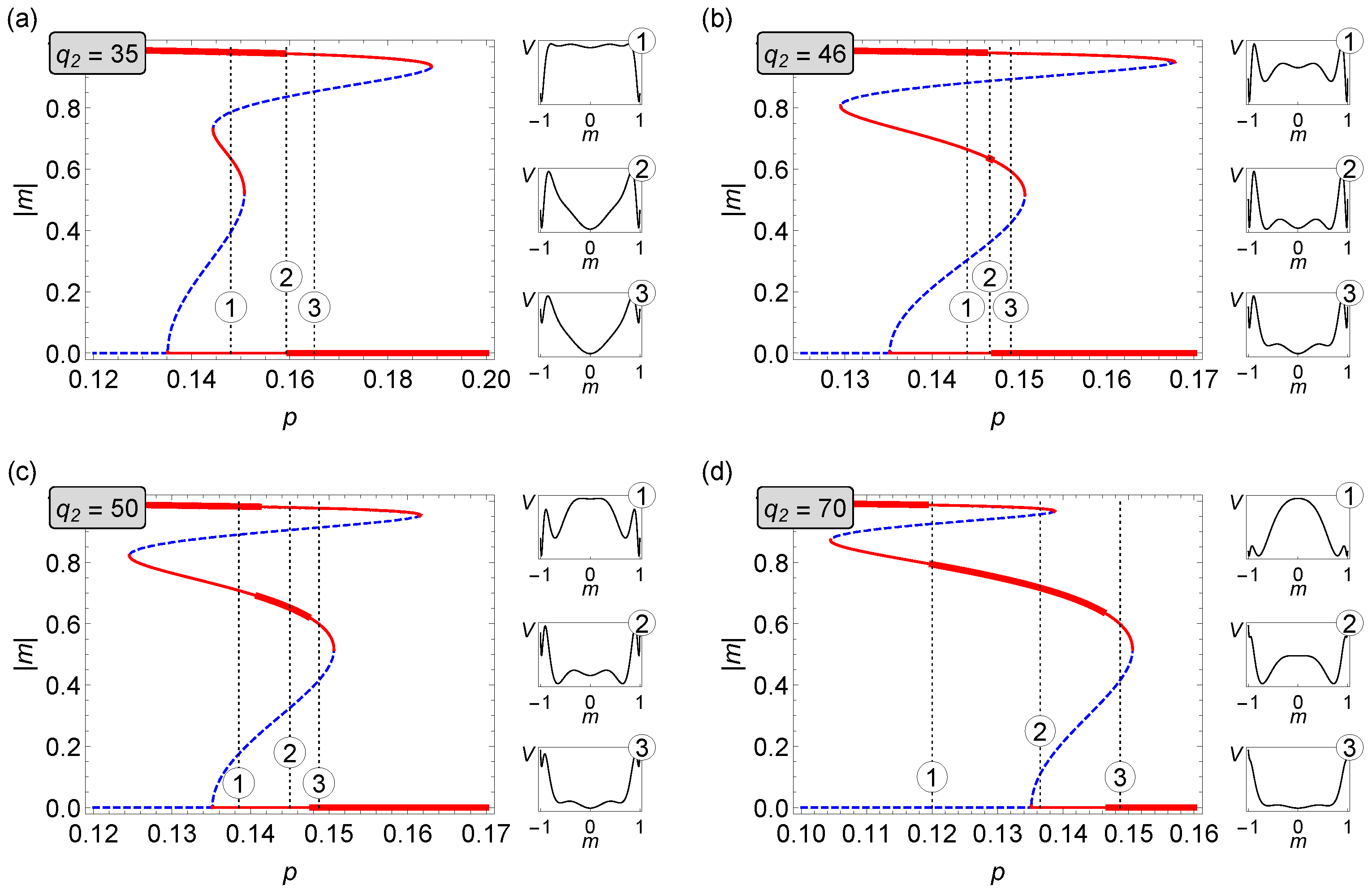
3.2.1. The Case
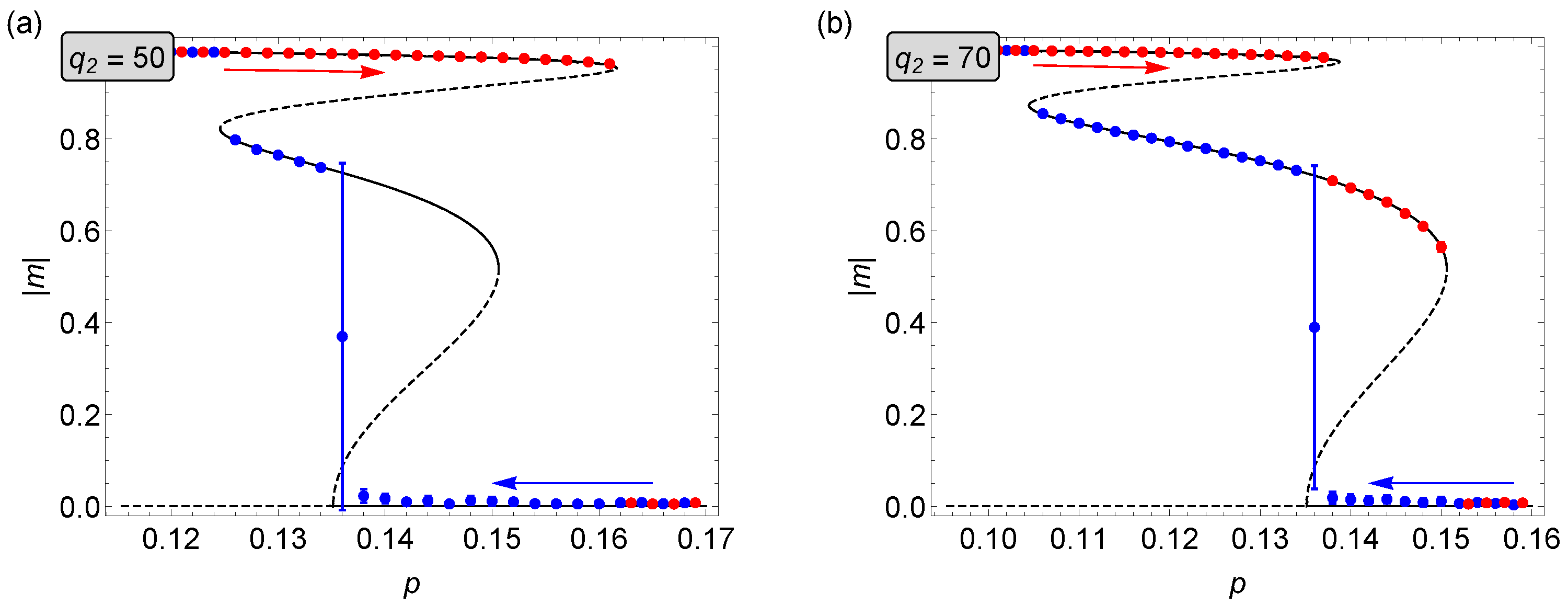
3.2.2. The Case
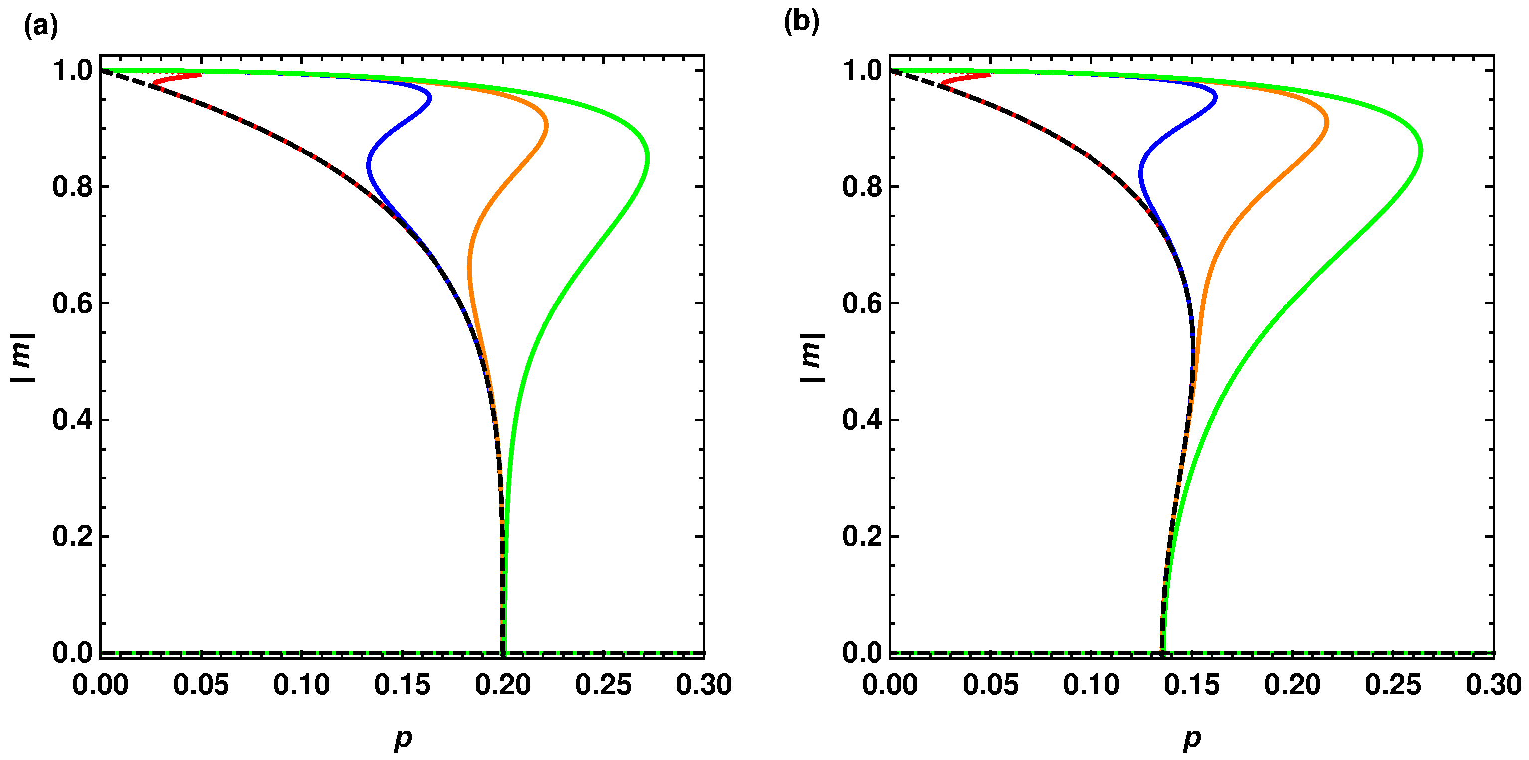
3.3. Limiting Behavior
4. Conclusions
Author Contributions
Funding
Conflicts of Interest
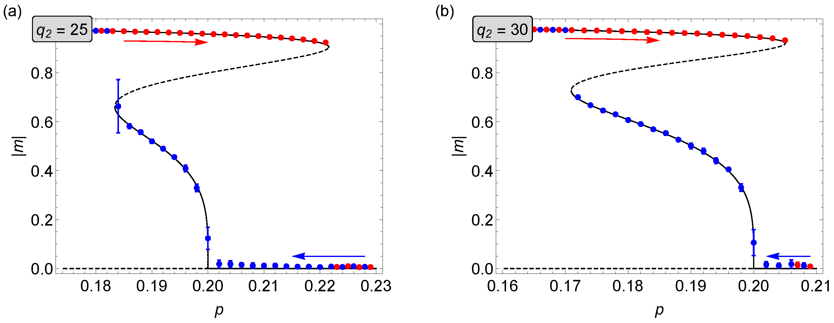
Appendix A. Monte-Carlo Simulations


References
- Castellano, C.; Fortunato, S.; Loreto, V. Statistical physics of social dynamics. Rev. Mod. Phys. 2009, 81, 591–646. [Google Scholar] [CrossRef]
- Sznajd-Weron, K.; Sznajd, J. Opinion evolution in closed community. Int. J. Mod. Phys. C 2000, 11, 1157–1165. [Google Scholar] [CrossRef]
- Liggett, T.M. Interactive Particle Systems; Springer: Berlin/Heidelberg, Germany, 2005. [Google Scholar] [CrossRef]
- Suchecki, K.; Eguíluz, V.M.; San Miguel, M. Voter model dynamics in complex networks: Role of dimensionality, disorder, and degree distribution. Phys. Rev. E 2005, 72, 036132. [Google Scholar] [CrossRef] [PubMed]
- Pereira, L.F.C.; Moreira, F.G.B. Majority-vote model on random graphs. Phys. Rev. E 2005, 71, 016123. [Google Scholar] [CrossRef] [PubMed]
- Watts, D.J. A simple model of global cascades on random networks. Proc. Natl. Acad. Sci. USA 2002, 99, 5766–5771. [Google Scholar] [CrossRef] [PubMed]
- Gleeson, J.P. Binary-State Dynamics on Complex Networks: Pair Approximation and Beyond. Phys. Rev. X 2013, 3, 021004. [Google Scholar] [CrossRef]
- Axelrod, R. The Complexity of Cooperation: Agent-Based Models of Competition and Collaboration; Princeton University Press: Princeton, NJ, USA, 1997. [Google Scholar] [CrossRef]
- Li, K.; Liang, H.; Kou, G.; Dong, Y. Opinion dynamics model based on the cognitive dissonance: An agent-based simulation. Inf. Fusion 2020, 56, 1–14. [Google Scholar] [CrossRef]
- Alatas, H.; Nurhimawan, S.; Asmat, F.; Hardhienata, H. Dynamics of an agent-based opinion model with complete social connectivity network. Chaos Solitons Fractals 2017, 101, 24–32. [Google Scholar] [CrossRef]
- González, M.C.; Lind, P.G.; Herrmann, H.J. System of Mobile Agents to Model Social Networks. Phys. Rev. Lett. 2006, 96, 088702. [Google Scholar] [CrossRef]
- Chmiel, A.; Sznajd-Weron, K. Phase transitions in the q-voter model with noise on a duplex clique. Phys. Rev. E 2015, 92, 052812. [Google Scholar] [CrossRef]
- Asch, S.E. Opinions and social pressure. Sci. Am. 1955, 193, 31–35. [Google Scholar] [CrossRef]
- Milgram, S.; Bickman, L.; Berkowitz, L. Note on the drawing power of crowds of different size. J. Personal. Soc. Psychol. 1969, 13, 79–82. [Google Scholar] [CrossRef]
- Elster, J. A Note on Hysteresis in the Social Sciences. Synthese 1976, 33, 371–391. [Google Scholar] [CrossRef]
- Centola, D.; Becker, J.; Brackbill, D.; Baronchelli, A. Experimental evidence for tipping points in social convention. Science 2018, 360, 1116–1119. [Google Scholar] [CrossRef] [PubMed]
- Nyczka, P.; Sznajd-Weron, K.; Cisło, J. Phase transitions in the q-voter model with two types of stochastic driving. Phys. Rev. E 2012, 86, 011105. [Google Scholar] [CrossRef]
- Jędrzejewski, A. Pair approximation for the q-voter model with independence on complex networks. Phys. Rev. E 2017, 95, 012307. [Google Scholar] [CrossRef]
- Boccaletti, S.; Bianconi, G.; Criado, R.; del Genio, C.I.; Gómez-Gardeñes, J.; Romance, M.; Sendiña-Nadal, I.; Wang, Z.; Zanin, M. The structure and dynamics of multilayer networks. Phys. Rep. 2014, 544, 1–122. [Google Scholar] [CrossRef]
- De Domenico, M.; Solé-Ribalta, A.; Gómez, S.; Arenas, A. Navigability of interconnected networks under random failures. Proc. Natl. Acad. Sci. USA 2014. [Google Scholar] [CrossRef]
- Gómez, S.; Díaz-Guilera, A.; Gómez-Gardeñes, J.; Pérez-Vicente, C.J.; Moreno, Y.; Arenas, A. Diffusion Dynamics on Multiplex Networks. Phys. Rev. Lett. 2013, 110, 028701. [Google Scholar] [CrossRef]
- Cencetti, G.; Battiston, F. Diffusive behavior of multiplex networks. New J. Phys. 2019, 21, 035006. [Google Scholar] [CrossRef]
- Granell, C.; Gómez, S.; Arenas, A. Dynamical Interplay between Awareness and Epidemic Spreading in Multiplex Networks. Phys. Rev. Lett. 2013, 111, 128701. [Google Scholar] [CrossRef] [PubMed]
- Choi, J.; Goh, K.I. Majority-vote dynamics on multiplex networks with two layers. New J. Phys. 2019, 21, 035005. [Google Scholar] [CrossRef]
- Artime, O.; Fernández-Gracia, J.; Ramasco, J.J.; San Miguel, M. Joint effect of ageing and multilayer structure prevents ordering in the voter model. Sci. Rep. 2017, 7, 7166. [Google Scholar] [CrossRef] [PubMed]
- Diakonova, M.; San Miguel, M.; Eguíluz, V.M. Absorbing and shattered fragmentation transitions in multilayer coevolution. Phys. Rev. E 2014, 89, 062818. [Google Scholar] [CrossRef] [PubMed]
- Gradowski, T.; Krawiecki, A. Pair approximation for the q-voter model with independence on multiplex networks. Phys. Rev. E 2020, 102, 022314. [Google Scholar] [CrossRef]
- Khare, A.; Christov, I.C.; Saxena, A. Successive phase transitions and kink solutions in ϕ8, ϕ10, and ϕ12 field theories. Phys. Rev. E 2014, 90, 023208. [Google Scholar] [CrossRef]
- Radosz, W.; Mielnik-Pyszczorski, A.; Brzezińska, M.; Sznajd-Weron, K. Q-voter model with nonconformity in freely forming groups: Does the size distribution matter? Phys. Rev. E 2017, 95, 062302. [Google Scholar] [CrossRef] [PubMed]
- Abramiuk, A.; Pawłowski, J.; Sznajd-Weron, K. Is Independence Necessary for a Discontinuous Phase Transition within the q-Voter Model? Entropy 2019, 21, 521. [Google Scholar] [CrossRef]
- Bar, A.; Mukamel, D. Mixed-order phase transition in a one-dimensional model. Phys. Rev. Lett. 2014, 112, 015701. [Google Scholar] [CrossRef]
- Fronczak, A.; Fronczak, P. Mixed-order phase transition in a minimal, diffusion based spin model. Phys. Rev. E 2016, 94, 012103. [Google Scholar] [CrossRef]
- Vieira, A.R.; Anteneodo, C. Threshold q-voter model. Phys. Rev. E 2018, 97, 052106. [Google Scholar] [CrossRef] [PubMed]
- Vieira, A.R.; Peralta, A.F.; Toral, R.; Miguel, M.S.; Anteneodo, C. Pair approximation for the noisy threshold q-voter model. Phys. Rev. E 2020, 101, 052131. [Google Scholar] [CrossRef] [PubMed]
- Kodama, M.; Kuwabara, M.; Seki, S. Successive phase-transition phenomena and phase diagram of the phosphatidylcholine-water system as revealed by differential scanning calorimetry. Biochim. Biophys. Acta (BBA) Biomembr. 1982, 689, 567–570. [Google Scholar] [CrossRef]
- Saito, M.; Watanabe, M.; Kurita, N.; Matsuo, A.; Kindo, K.; Avdeev, M.; Jeschke, H.O.; Tanaka, H. Successive phase transitions and magnetization plateau in the spin-1 triangular-lattice antiferromagnet Ba2La2NiTe2O12 with small easy-axis anisotropy. Phys. Rev. B 2019, 100, 064417. [Google Scholar] [CrossRef]
- Oestereich, A.L.; Pires, M.A.; Crokidakis, N. Three-state opinion dynamics in modular networks. Phys. Rev. E 2019, 100, 032312. [Google Scholar] [CrossRef]
- Jȩdrzejewski, A.; Chmiel, A.; Sznajd-Weron, K. Oscillating hysteresis in the q-neighbor Ising model. Phys. Rev. E 2015, 92, 052105. [Google Scholar] [CrossRef]
- Chmiel, A.; Sienkiewicz, J.; Sznajd-Weron, K. Tricriticality in the q-neighbor Ising model on a partially duplex clique. Phys. Rev. E 2017, 96, 062137. [Google Scholar] [CrossRef]


| Property | Monoplex | Symmetric Duplex | Asymmetric Duplex |
|---|---|---|---|
| parameters | p, q | p, q | p, , |
| continuous PT | , | ||
| discontinuous PT | , , also observed for and specific | ||
| successive PTs | not observed | not observed | for first discontinuous PT and then continuous one; for two discontinuous PT |
| mixed-order PT | not observed | not observed | observed for and |
© 2020 by the authors. Licensee MDPI, Basel, Switzerland. This article is an open access article distributed under the terms and conditions of the Creative Commons Attribution (CC BY) license (http://creativecommons.org/licenses/by/4.0/).
Share and Cite
Chmiel, A.; Sienkiewicz, J.; Fronczak, A.; Fronczak, P. A Veritable Zoology of Successive Phase Transitions in the Asymmetric q-Voter Model on Multiplex Networks. Entropy 2020, 22, 1018. https://doi.org/10.3390/e22091018
Chmiel A, Sienkiewicz J, Fronczak A, Fronczak P. A Veritable Zoology of Successive Phase Transitions in the Asymmetric q-Voter Model on Multiplex Networks. Entropy. 2020; 22(9):1018. https://doi.org/10.3390/e22091018
Chicago/Turabian StyleChmiel, Anna, Julian Sienkiewicz, Agata Fronczak, and Piotr Fronczak. 2020. "A Veritable Zoology of Successive Phase Transitions in the Asymmetric q-Voter Model on Multiplex Networks" Entropy 22, no. 9: 1018. https://doi.org/10.3390/e22091018
APA StyleChmiel, A., Sienkiewicz, J., Fronczak, A., & Fronczak, P. (2020). A Veritable Zoology of Successive Phase Transitions in the Asymmetric q-Voter Model on Multiplex Networks. Entropy, 22(9), 1018. https://doi.org/10.3390/e22091018