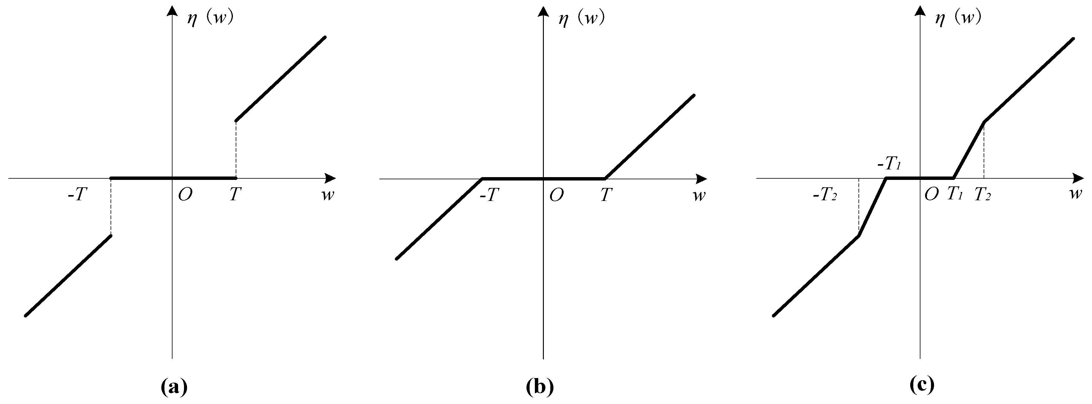
Figure 1.
Schematic of three wavelet threshold functions. (a) hard thresholding function, (b) soft thresholding function, (c) semi-soft thresholding function.
Figure 1.
Schematic of three wavelet threshold functions. (a) hard thresholding function, (b) soft thresholding function, (c) semi-soft thresholding function.
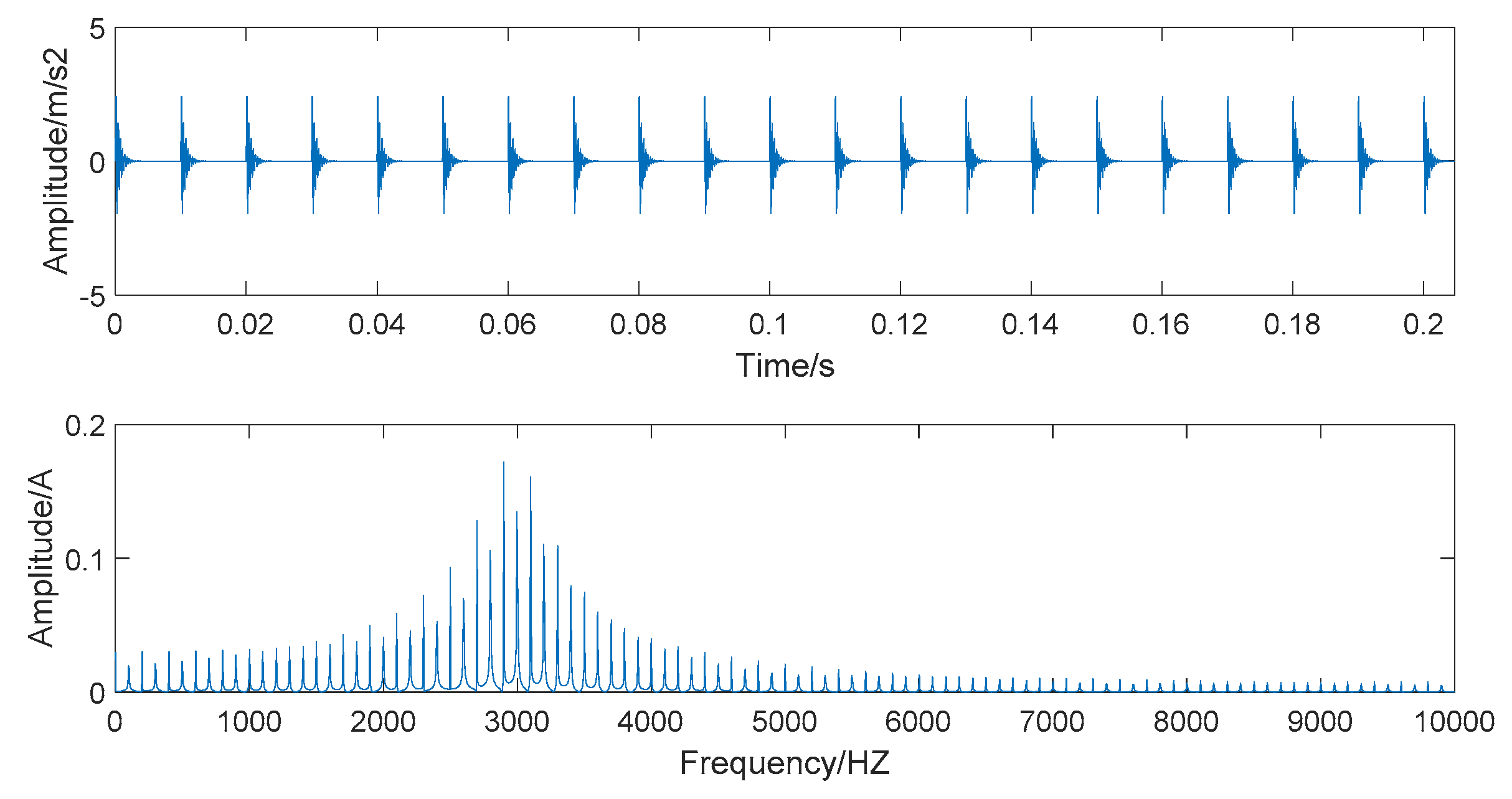
Figure 2.
The time domain and frequency domain chart of noiseless simulated signal.
Figure 2.
The time domain and frequency domain chart of noiseless simulated signal.
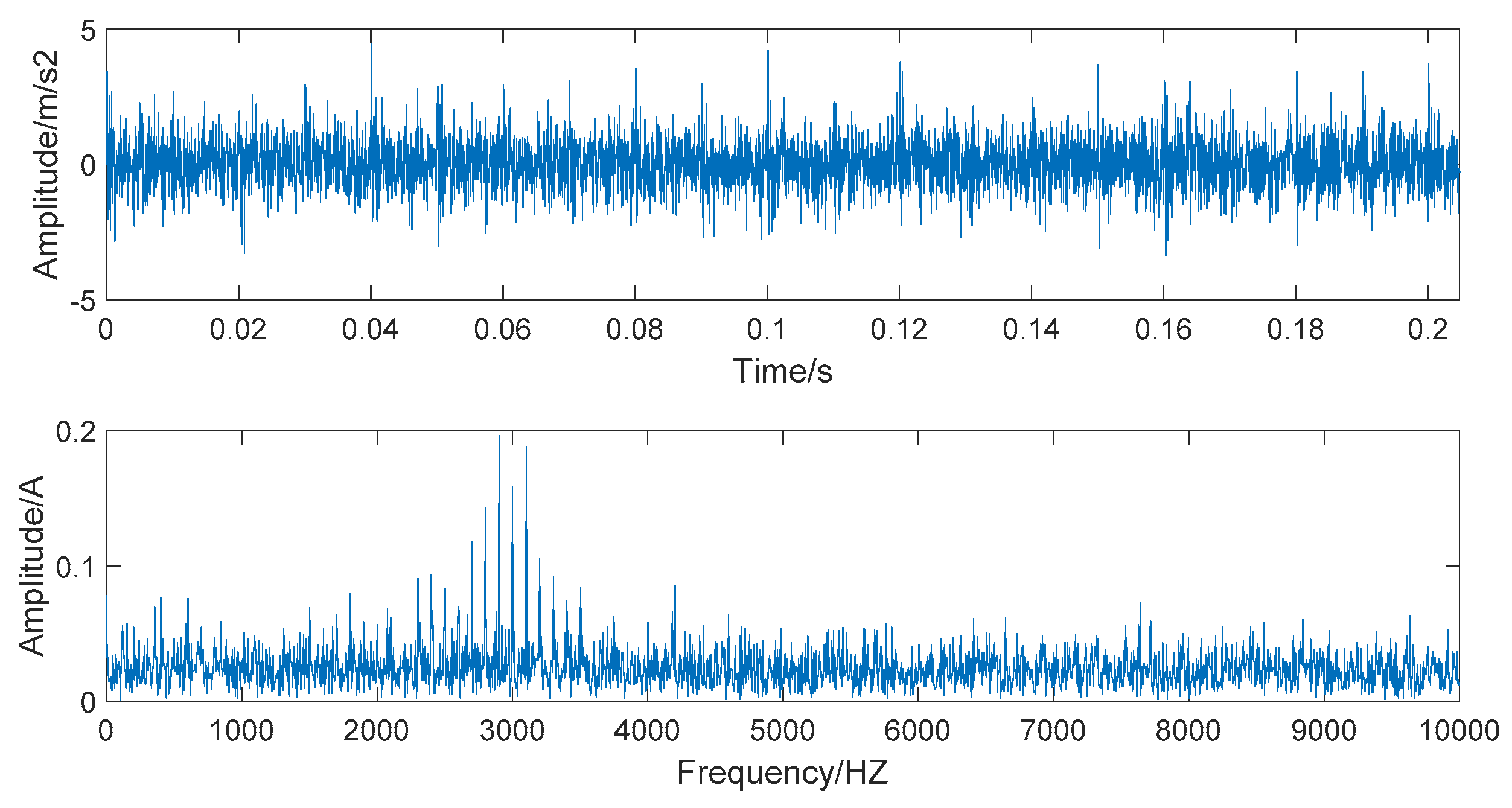
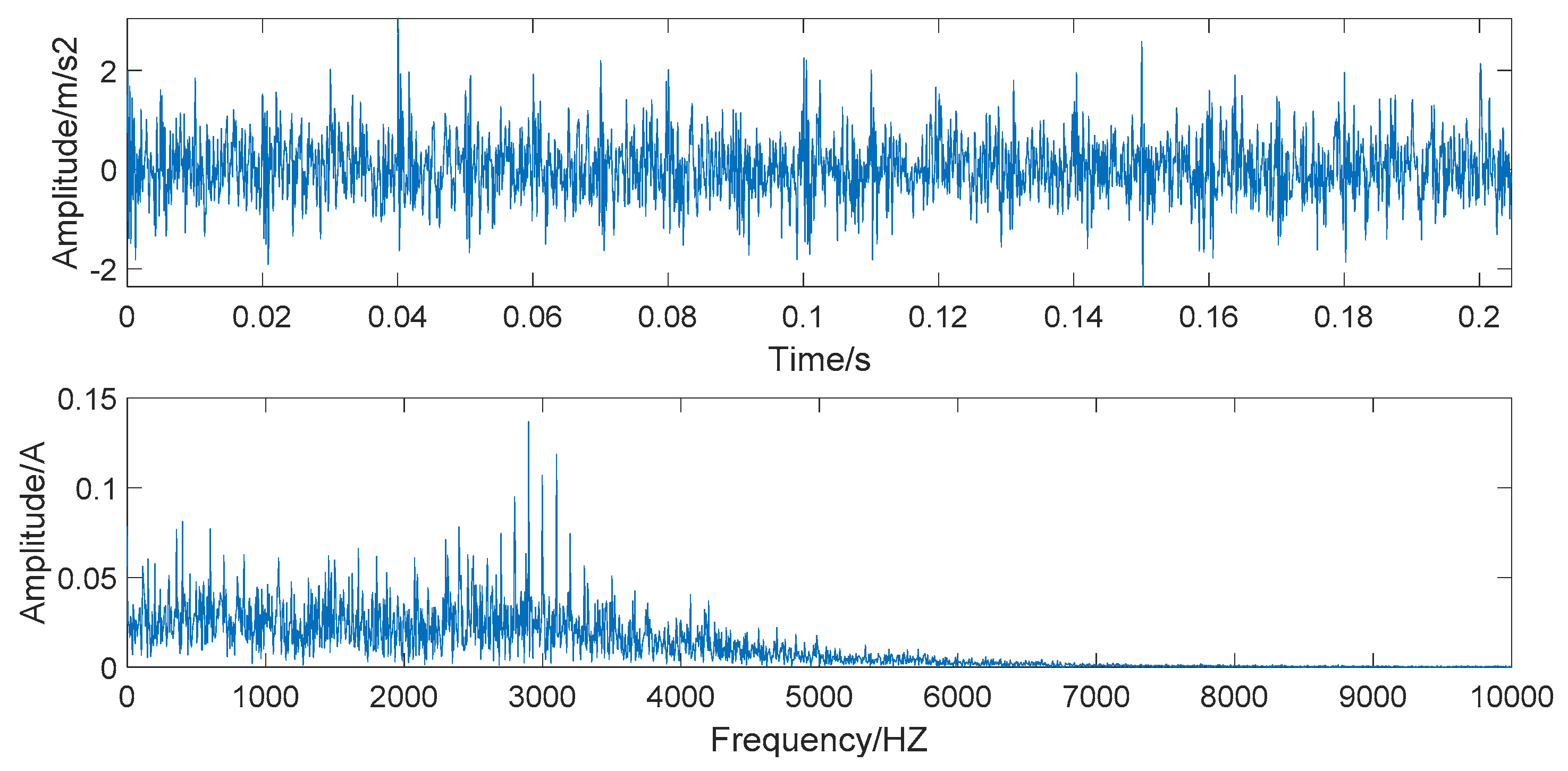
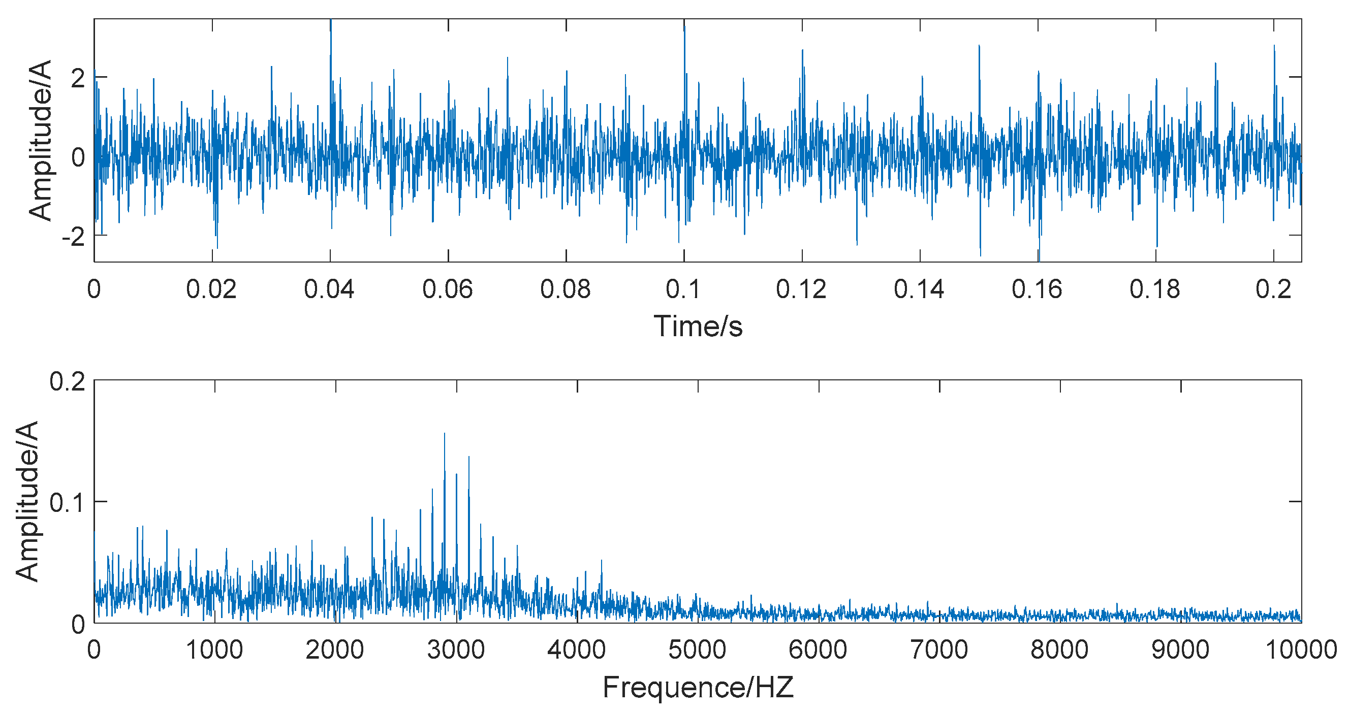
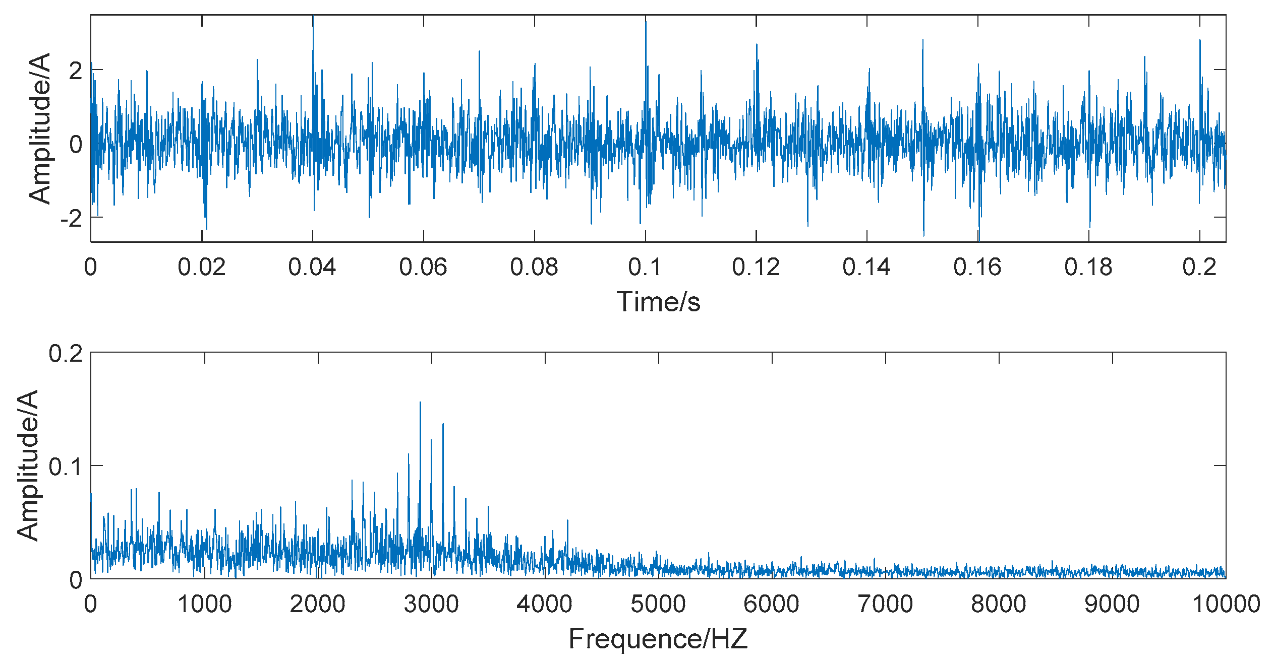
Figure 3.
The time domain and frequency domain chart of noise-added simulated signal.
Figure 3.
The time domain and frequency domain chart of noise-added simulated signal.
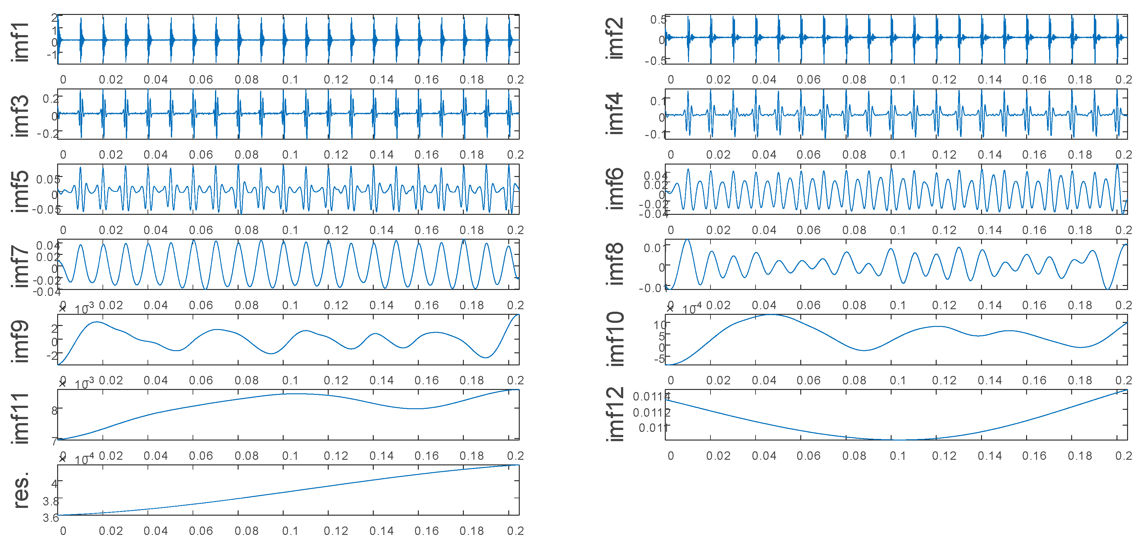
Figure 4.
Decomposition result of the noiseless simulated signal.
Figure 4.
Decomposition result of the noiseless simulated signal.
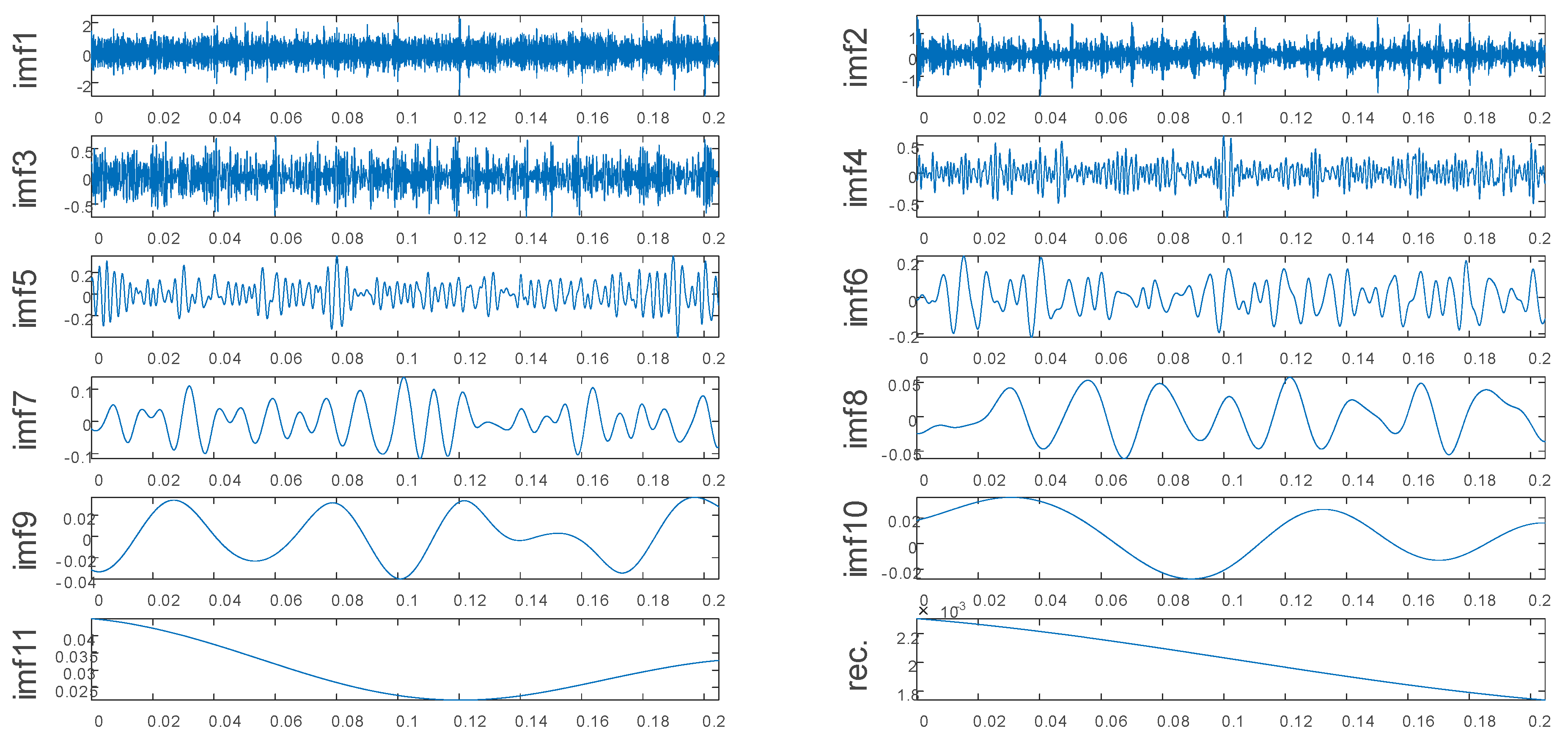
Figure 5.
Decomposition result of the noise-added simulated signal.
Figure 5.
Decomposition result of the noise-added simulated signal.
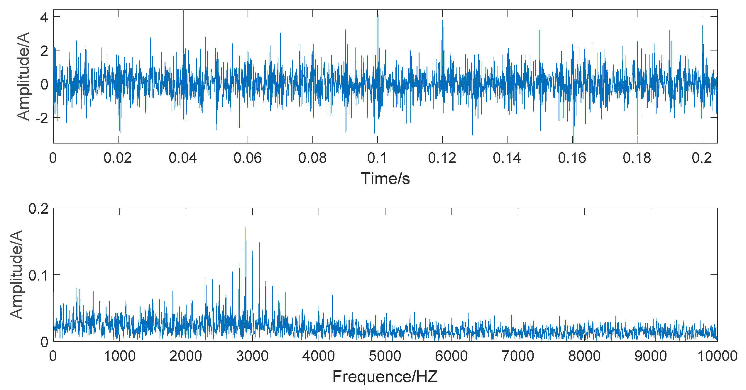
Figure 6.
The time domain and frequency domain chart of simulated signal after ensemble empirical mode decomposition (EEMD) forced denoising.
Figure 6.
The time domain and frequency domain chart of simulated signal after ensemble empirical mode decomposition (EEMD) forced denoising.
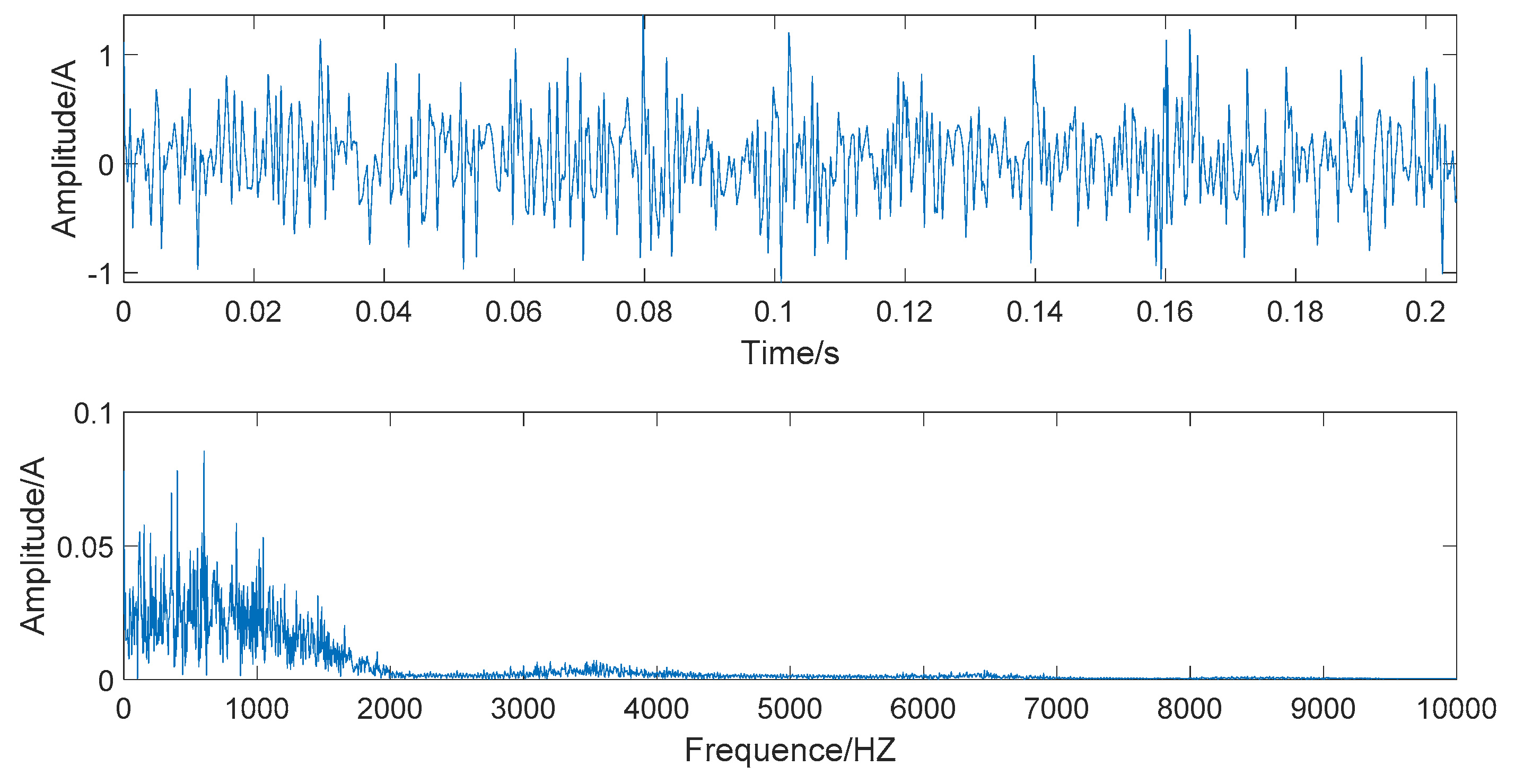
Figure 7.
The time domain and frequency domain chart after wavelet threshold denoising.
Figure 7.
The time domain and frequency domain chart after wavelet threshold denoising.
Figure 8.
The time domain and frequency domain chart of the signal denoised by the EEMD- wavelet hard threshold (WHT).
Figure 8.
The time domain and frequency domain chart of the signal denoised by the EEMD- wavelet hard threshold (WHT).
Figure 9.
The time domain and frequency domain chart of the signal denoised by the EEMD- wavelet soft threshold (WST).
Figure 9.
The time domain and frequency domain chart of the signal denoised by the EEMD- wavelet soft threshold (WST).
Figure 10.
The time domain and frequency domain chart of the signal denoised by the EMD- wavelet semi-soft threshold (WSST).
Figure 10.
The time domain and frequency domain chart of the signal denoised by the EMD- wavelet semi-soft threshold (WSST).
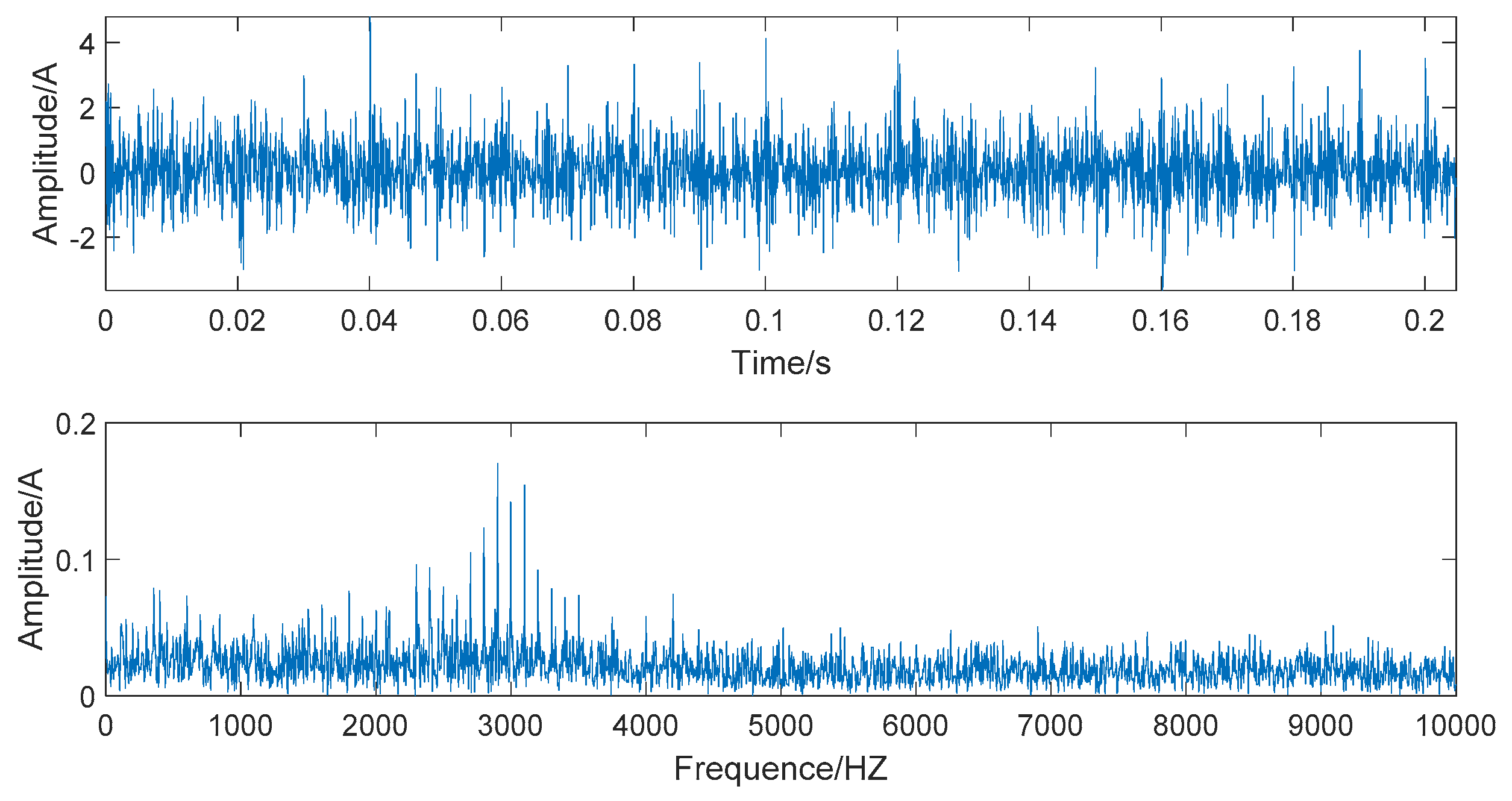
Figure 11.
The time domain and frequency domain chart of the signal denoised by the EEMD-WSST.
Figure 11.
The time domain and frequency domain chart of the signal denoised by the EEMD-WSST.
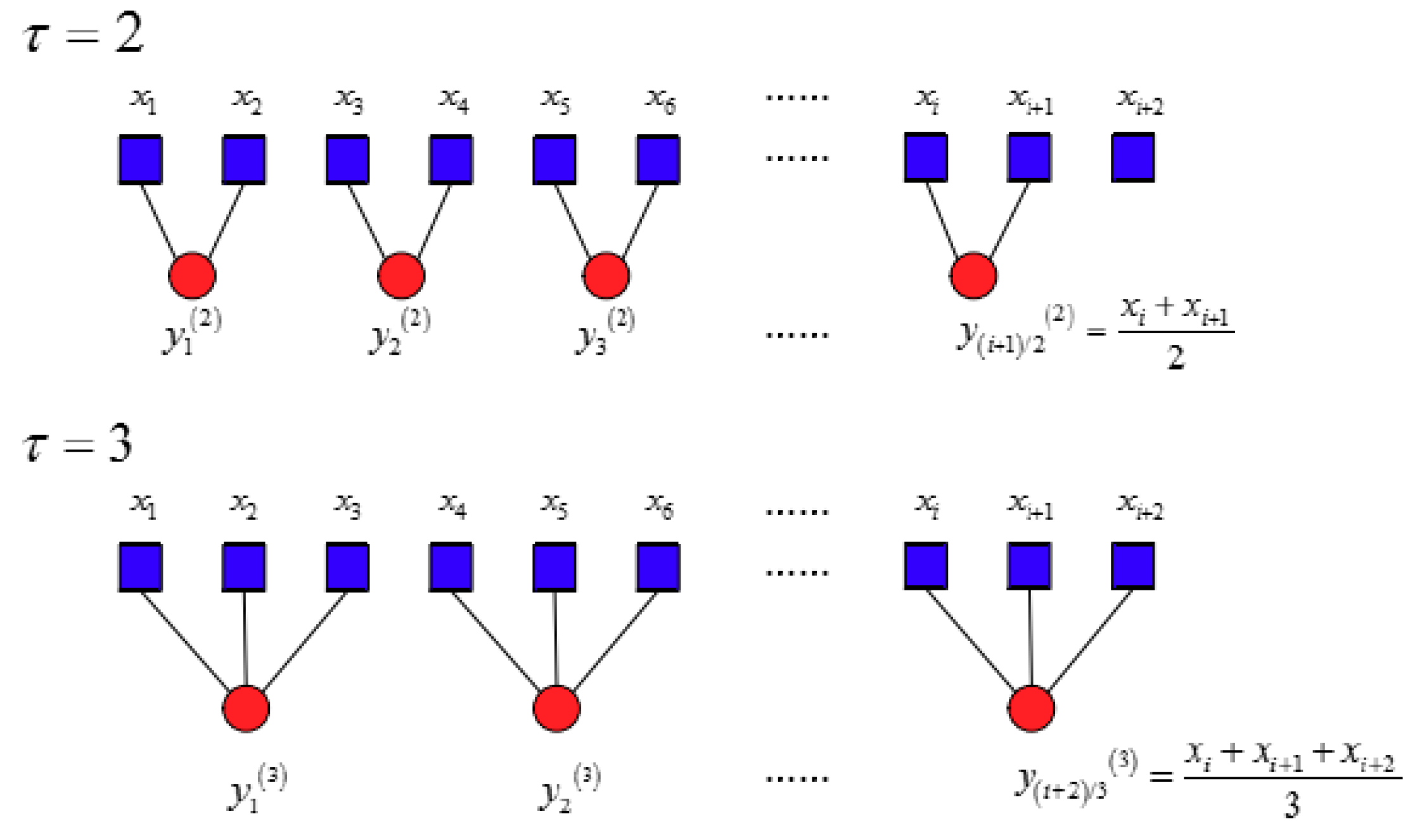
Figure 12.
Schematic of the coarse-graining process at and .
Figure 12.
Schematic of the coarse-graining process at and .
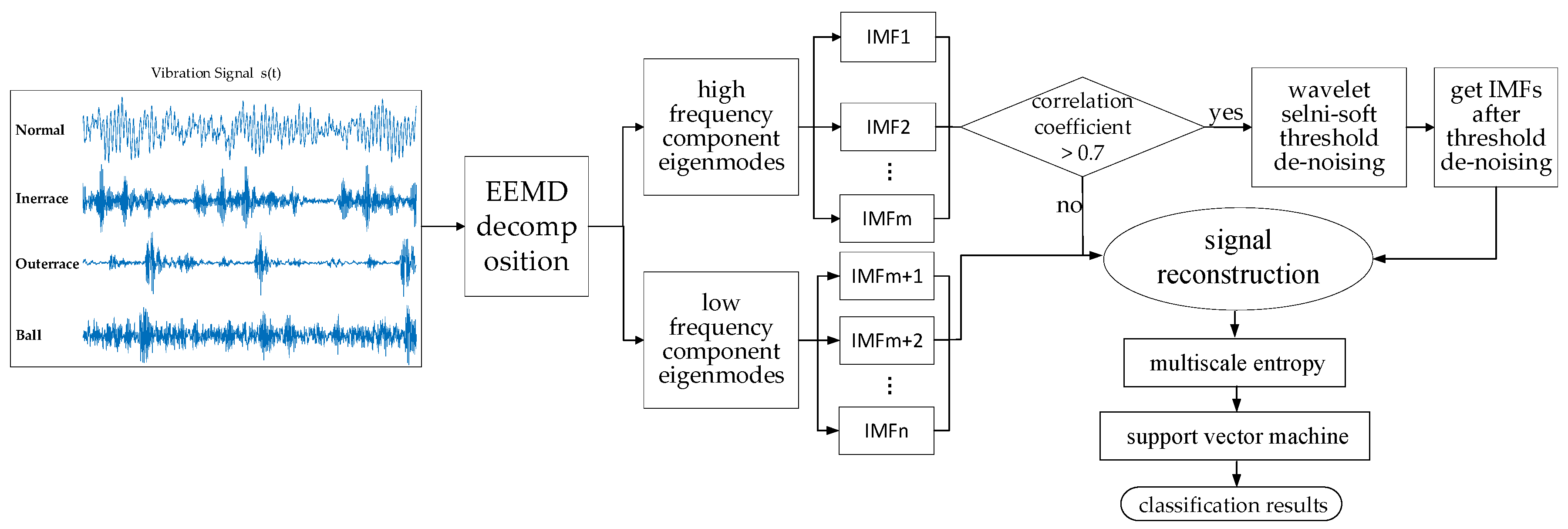
Figure 13.
Flow of the presented model.
Figure 13.
Flow of the presented model.
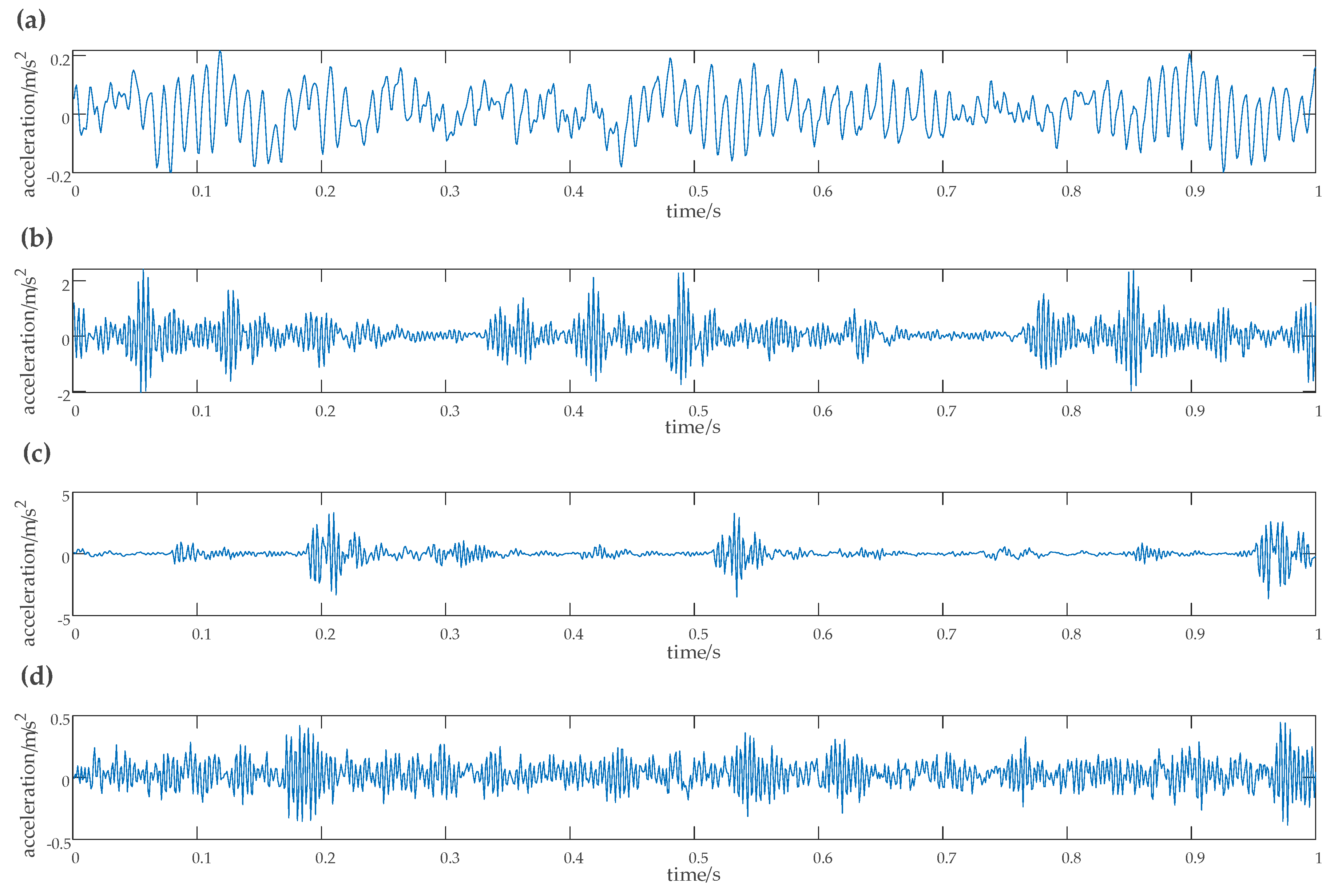
Figure 14.
Vibration signal time diagram of the SKF6203 bearing. (a) Amplitude of vibration acceleration of the original signal, (b) amplitude of vibration acceleration of the inner race fault signal, (c) amplitude of vibration acceleration of the outer race fault signal, (d) amplitude of vibration acceleration of the rolling element fault signal.
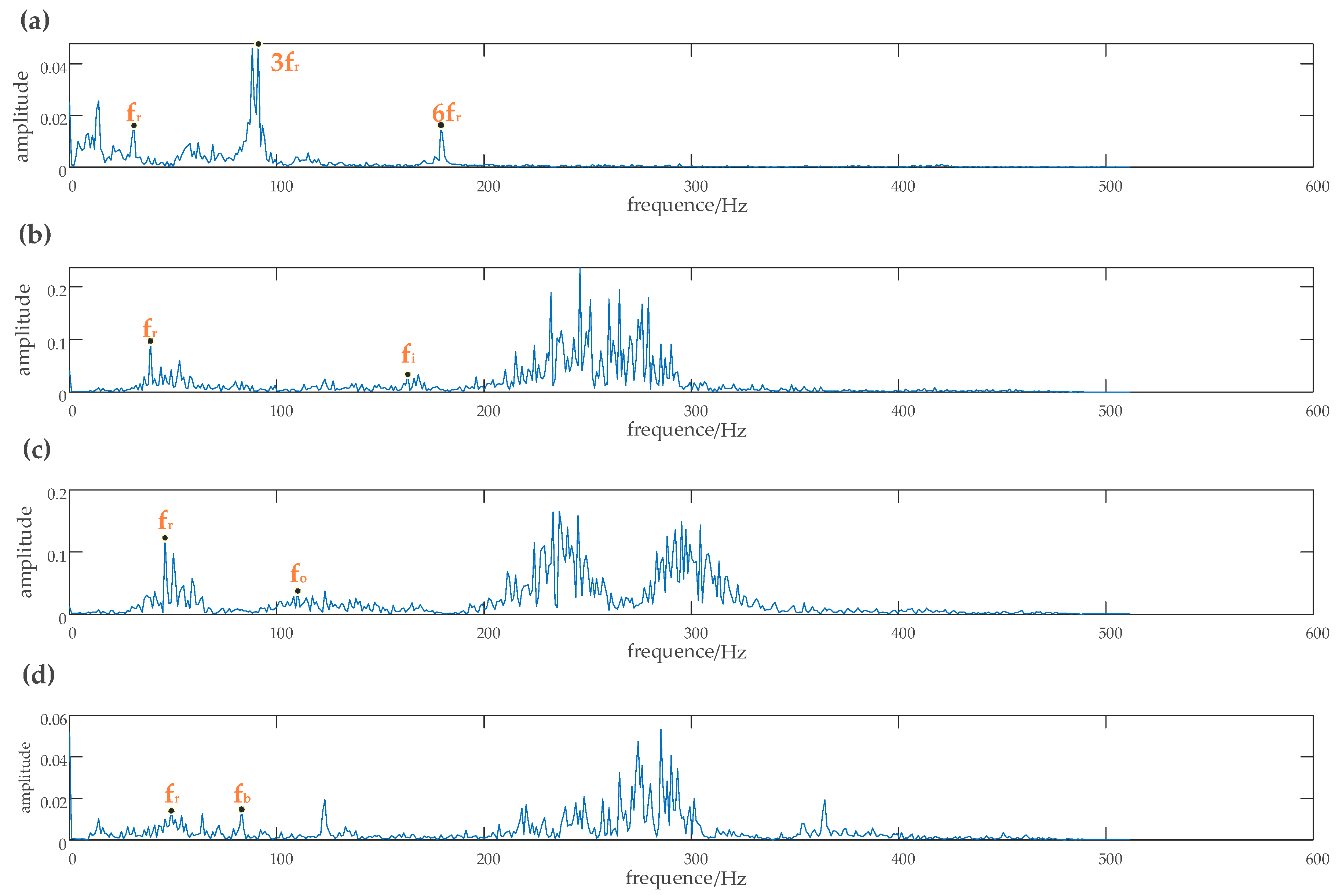
Figure 15.
Vibration signal Spectrum diagram of the SKF6203 bearing. (a) Spectrum of the raw signal, (b) spectrum of the inner race fault signal, (c) spectrum of the outer race fault signal, (d) spectrum of the ball fault signal.
Figure 15.
Vibration signal Spectrum diagram of the SKF6203 bearing. (a) Spectrum of the raw signal, (b) spectrum of the inner race fault signal, (c) spectrum of the outer race fault signal, (d) spectrum of the ball fault signal.
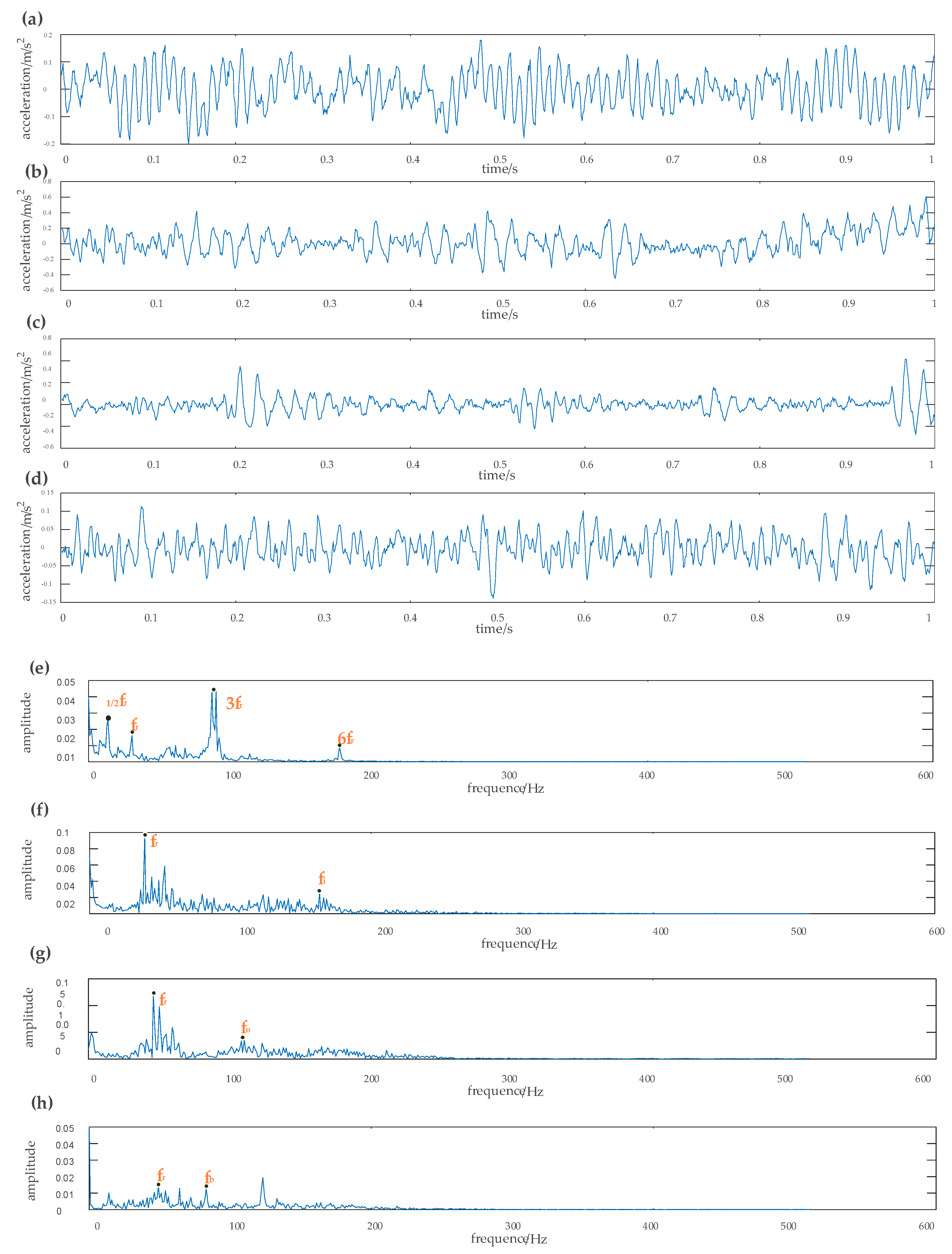
Figure 16.
Time-domain and frequency waveform of different signals obtained by EEMD-WSST. (a) Amplitude of vibration acceleration of the original signal, (b) amplitude of vibration acceleration of the inner race fault signal, (c) amplitude of vibration acceleration of the outer race fault signal, (d) amplitude of vibration acceleration of the ball fault signal, (e) spectrum of the raw signal, (f) spectrum of the inner race fault signal, (g) spectrum of the outer race fault signal, (h) spectrum of the ball fault signal.
Figure 17.
The results of the MSE analysis. (a) MSE curve of the MSE-EEMD, (b) MSE curve of the MSE-EEMD-WSST, (c) MSE scatter diagrams of the MSE-EEMD, (d) MSE scatter diagrams of the MSE-EEMD-WSST.
Figure 17.
The results of the MSE analysis. (a) MSE curve of the MSE-EEMD, (b) MSE curve of the MSE-EEMD-WSST, (c) MSE scatter diagrams of the MSE-EEMD, (d) MSE scatter diagrams of the MSE-EEMD-WSST.
Figure 18.
Classification results of fault identification with different characteristics of case 1. (a) Classification result of the original fault signals and sample entropy (SE-OFS), (b) classification result of the SE-EMD, (c) classification result of the SE-EEMD, (d) classification result of the MSE-OFS, (e) classification result of the MSE-EMD, (f) Classification result of the MSE-EEMD-WSST.
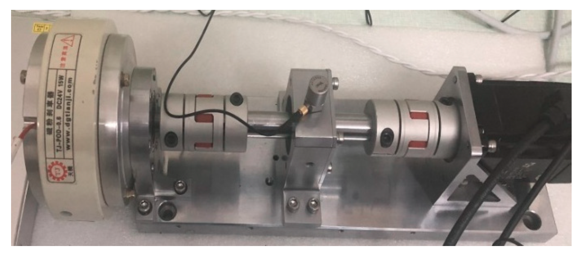
Figure 19.
The rotating machinery test bed.
Figure 19.
The rotating machinery test bed.
Figure 20.
The waveform of the vibration of different fault types. (a) Amplitude of vibration acceleration of the original signal, (b) amplitude of vibration acceleration of the inner race fault signal, (c) amplitude of vibration acceleration of the outer race fault signal, (d) amplitude of vibration acceleration of the rolling element fault signal, (e) spectrum of the original signal, (f) spectrum of the inner race fault signal, (g) spectrum of the outer race fault signal, (h) spectrum of the rolling element fault signal.
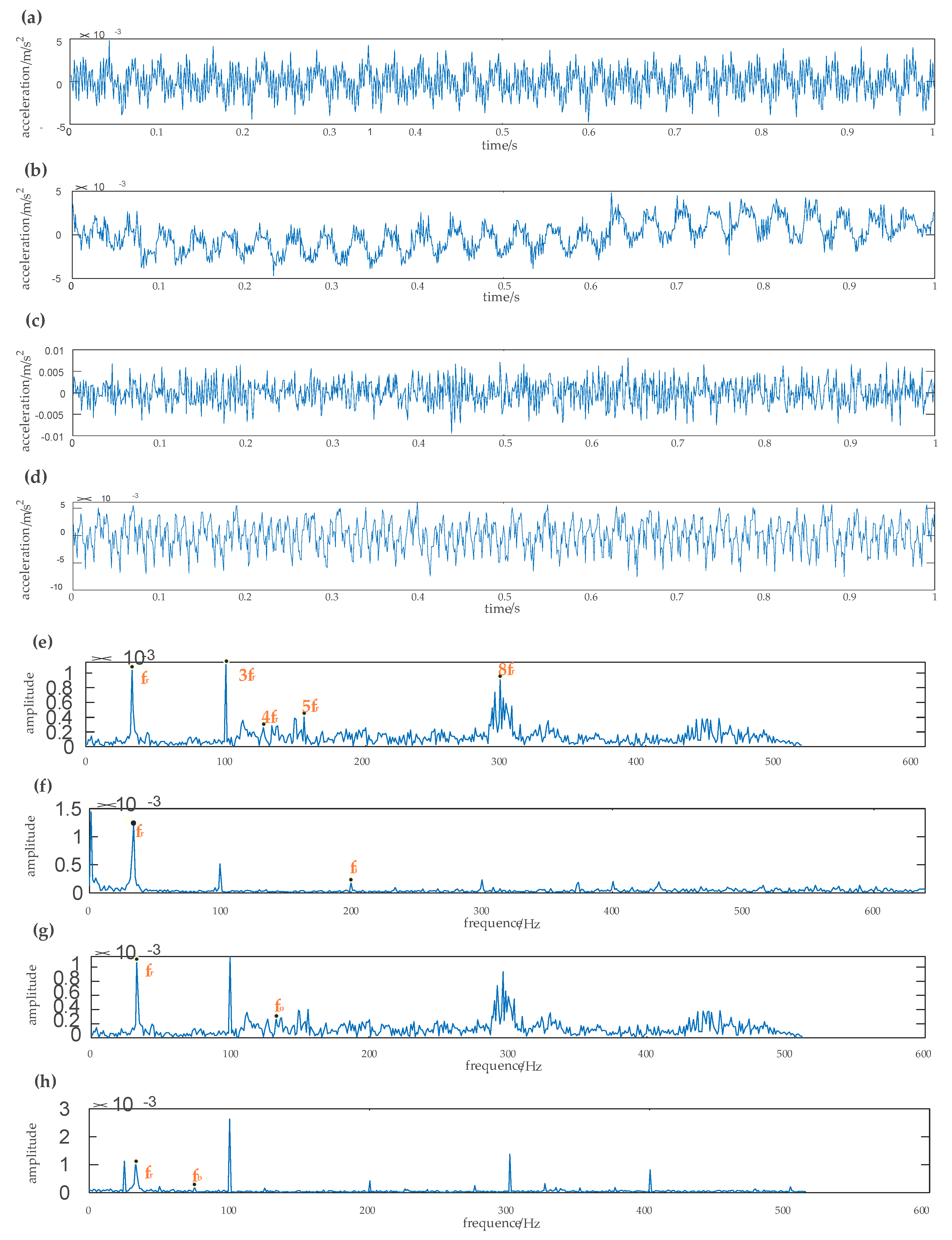
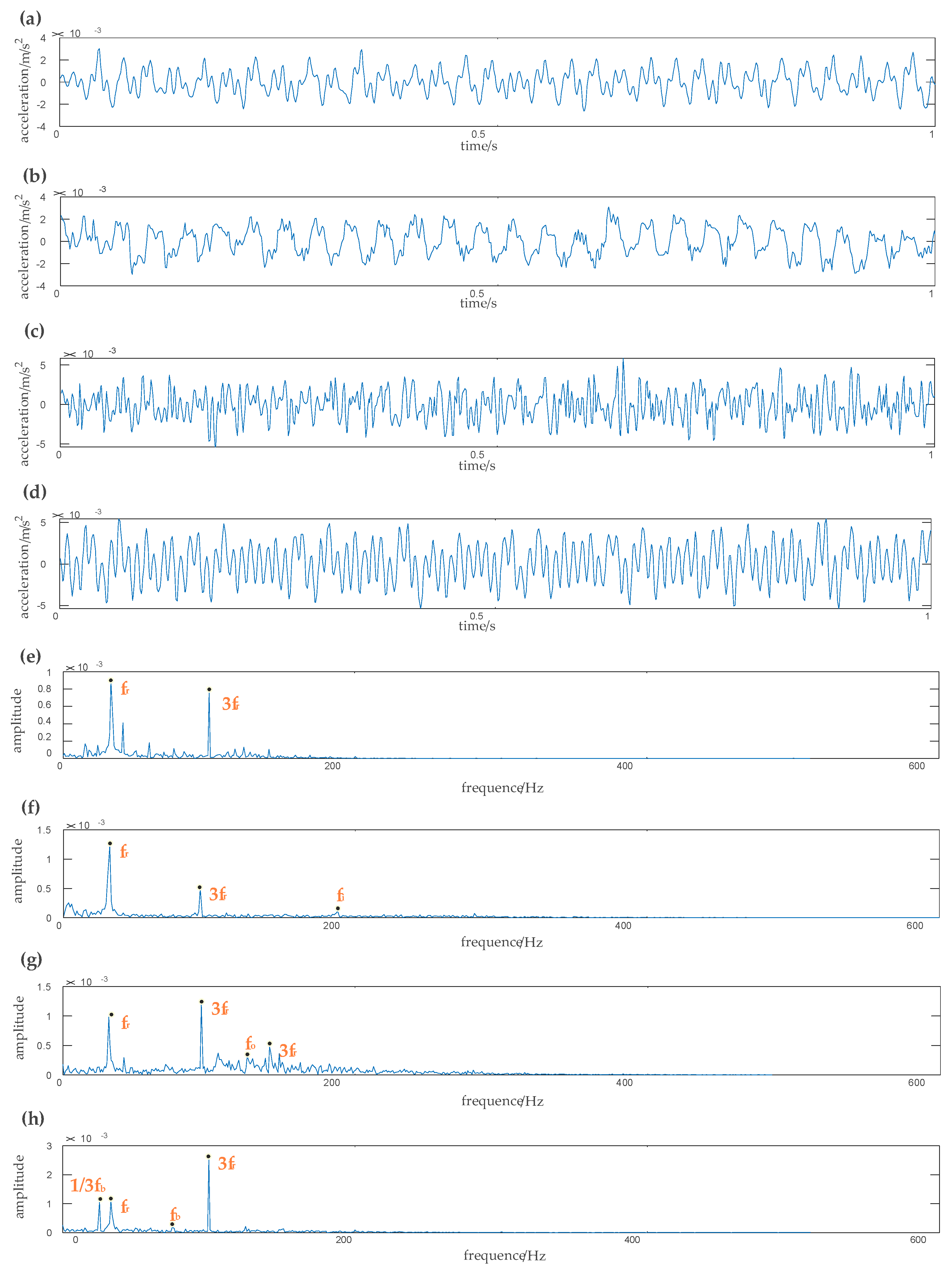
Figure 21.
Time-domain and frequency waveform of different signals obtained by EEMD-WSST. (a) Amplitude of vibration acceleration of original signal, (b) amplitude of vibration acceleration of the inner race fault signal, (c) amplitude of vibration acceleration of the outer race fault signal, (d) amplitude of vibration acceleration of the rolling element fault signal, (e) spectrum of the original signal, (f) spectrum of the inner race fault signal, (g) spectrum of the outer race fault signal, (h) spectrum of the rolling element fault signal.
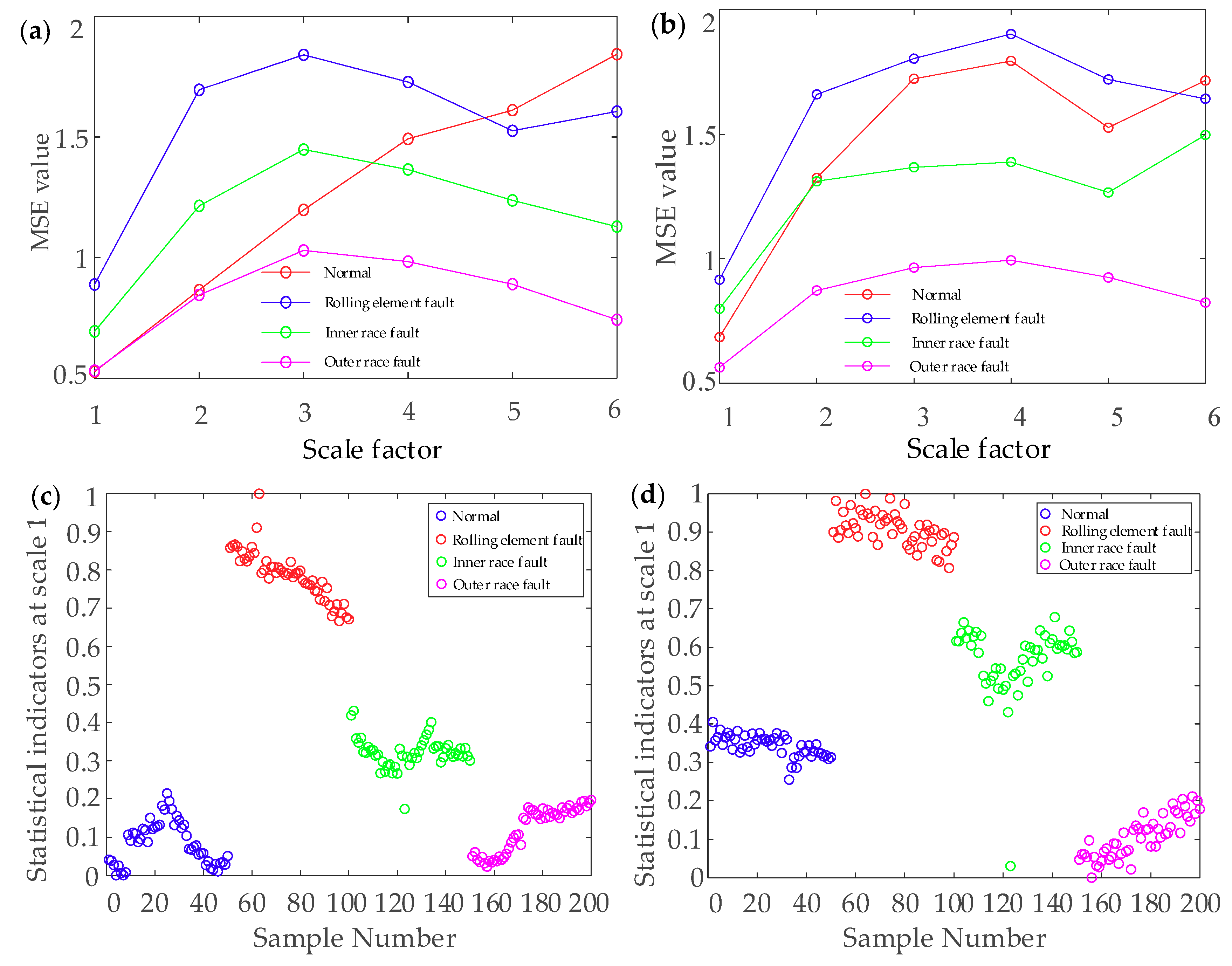
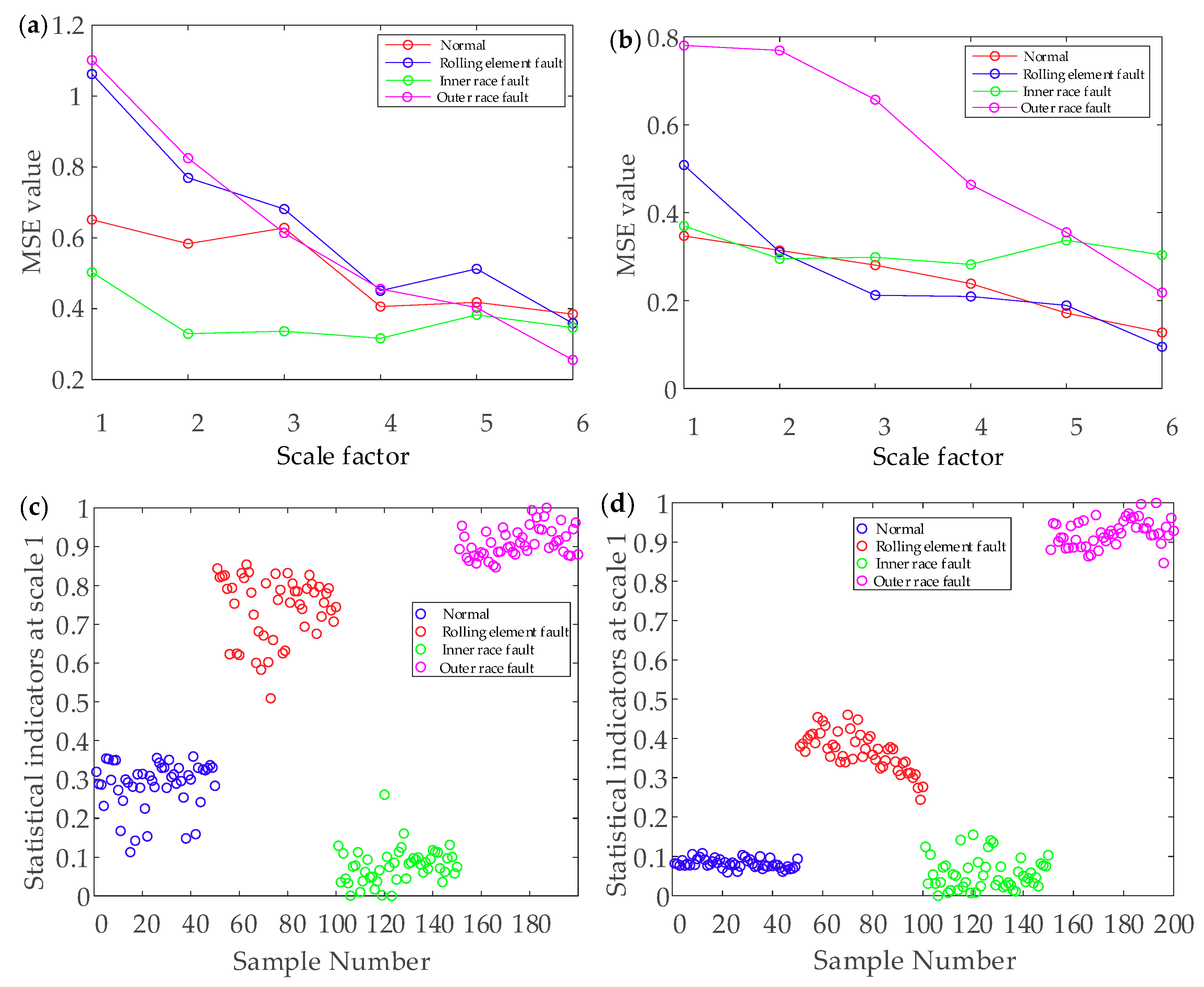
Figure 22.
The result of MSE analysis. (a) MSE curve of the MSE-EEMD. (b) MSE curve of the MSE-EEMD-WSST. (c) MSE scatter diagrams of the MSE-EEMD. (d) MSE scatter diagrams of the MSE-EEMD-WSST.
Figure 22.
The result of MSE analysis. (a) MSE curve of the MSE-EEMD. (b) MSE curve of the MSE-EEMD-WSST. (c) MSE scatter diagrams of the MSE-EEMD. (d) MSE scatter diagrams of the MSE-EEMD-WSST.
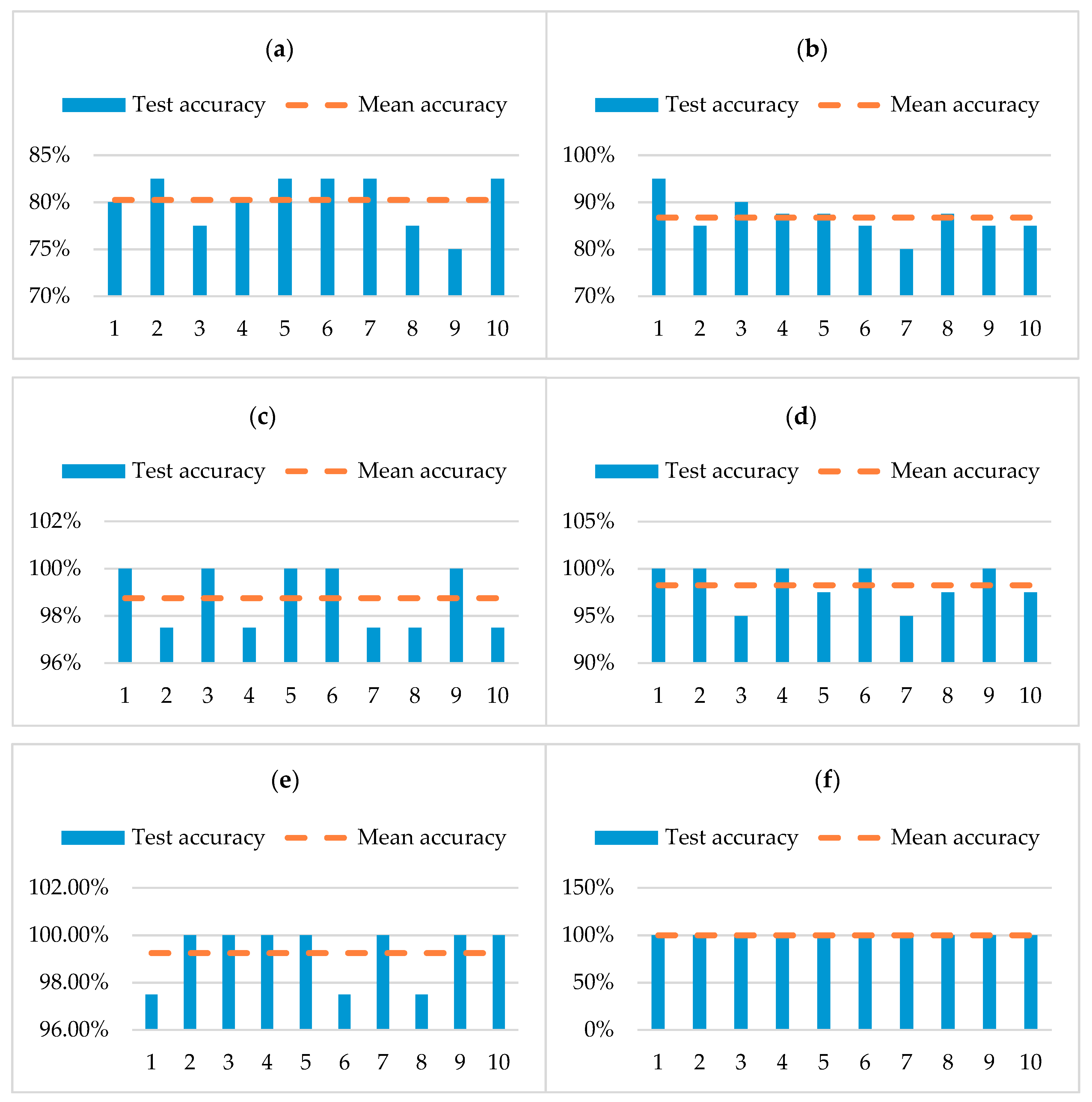
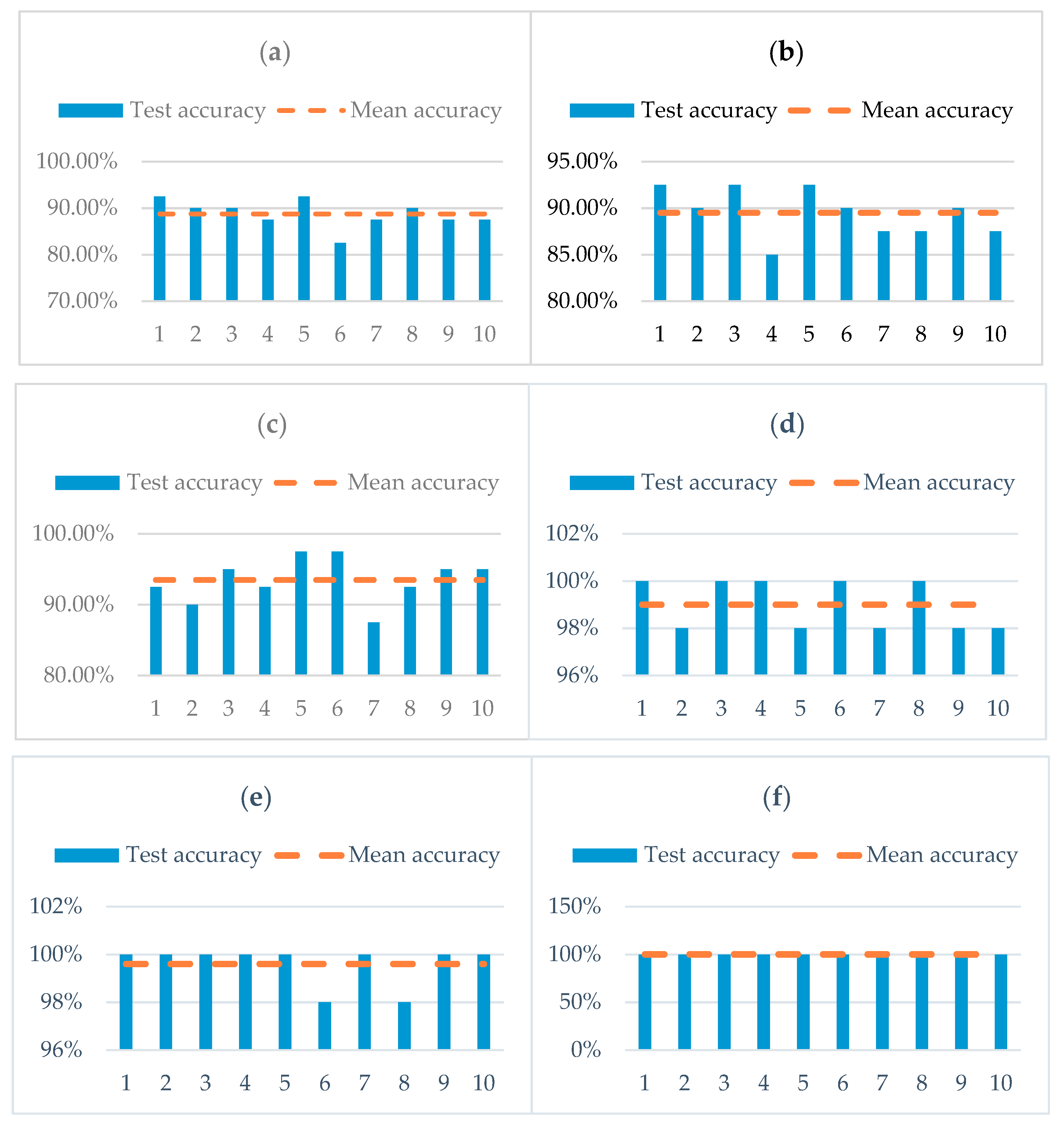
Figure 23.
Classification results of fault identification with different characteristics of case 2. (a) Classification result of the SE-OFS, (b) classification result of the SE-EMD, (c) classification result of the SE-EEMD, (d) classification result of the MSE-OFS, (e) classification result of the MSE-EMD, (f) classification result of the MSE-EEMD-WSST.
Table 1.
Correlation degree based on Pearson correlation coefficients.
Table 1.
Correlation degree based on Pearson correlation coefficients.
| Pearson Correlation Coefficient | Correlation Degree |
|---|
| 0.7–1.0 | strong linear correlation |
| 0.4–0.7 | significant correlation |
| 0–0.4 | weak linear correlation |
Table 2.
The correlation analysis results of intrinsic mode functions (IMFs).
Table 2.
The correlation analysis results of intrinsic mode functions (IMFs).
| IMFs | IMF1 | IMF2 | IMF3 | IMF4 | IMF5 | IMF6 | IMF7 | IMF8 | IMF9 | IMF10 | IMF11/Rec. | Rec. |
|---|
| EMD correlation coefficient | 0.7612 | 0.5694 | 0.3336 | 0.2584 | 0.1726 | 0.1319 | 0.092 | 0.0483 | 0.0261 | 0.0310 | 0.0204 | 0.0157 |
| EEMD correlation coefficient | 0.7142 | 0.531 | 0.2981 | 0.1891 | 0.1469 | 0.1026 | 0.0806 | 0.0387 | 0.0151 | 0.0217 | 0.0112 | |
Table 3.
The evaluation results of the denoising methods.
Table 3.
The evaluation results of the denoising methods.
| | Wavelet Denoising | EMD Forced Denoising | EEMD Forced Denoising | EEMD-WHT | EEMD-WST | EMD-WSST | EEMD-WSST |
|---|
| RMSE | 1.7239 | 1.3685 | 1.3560 | 1.5656 | 1.5738 | 1.2203 | 1.1196 |
| SNR | 0.6290 | 2.6342 | 2.7145 | 1.4655 | 1.4206 | 3.6300 | 4.3782 |
Table 4.
The details of the four conditions.
Table 4.
The details of the four conditions.
| Working Condition | Defect Size (Inches) | Number of Training Data Points | Number of Testing Data Points | Label of Classification |
|---|
| Normal | 0 | 40 | 10 | 1 |
| Inner race | 0.021 | 40 | 10 | 2 |
| Outer race | 0.021 | 40 | 10 | 3 |
| Rolling element | 0.021 | 40 | 10 | 4 |
Table 5.
Fault identification results of different feature extraction methods.
Table 5.
Fault identification results of different feature extraction methods.
| Feature Set | Total | Normal | Inner Race Fault | Outer Race Fault | Rolling Element Fault | Average Classification Accuracy (%) |
|---|
| Misclassification Number | Misclassification Number | Misclassification Number | Misclassification Number |
|---|
| SE-OFS | 79 | 4 | 75 | 0 | 0 | 80.25% |
| SE-EMD | 52 | 25 | 1 | 25 | 1 | 86.75% |
| SE-EEMD | 5 | 0 | 5 | 0 | 0 | 98.75% |
| MSE-OFS | 7 | 0 | 3 | 4 | 0 | 98.25% |
| MSE-EMD | 3 | 0 | 3 | 0 | 0 | 99.25% |
| MSE-EEMD-WSST | 0 | 0 | 0 | 0 | 0 | 100% |
Table 6.
Comparison between a number of other techniques. Support vector machine (SVM), higher order statistics analysis (HOSA), principal components analysis (PCA), artificial neural networks (ANN), ensemble empirical mode decomposition (EEMD), inter-cluster distance (ICD), multiscale permutation entropy (MPE), stacked sparse denoising autoencoder (SSDAE), fault diagnosis model based on ensemble deep neural network and convolution neural networks (CNNEPDNN), Feature-to-Feature- and Feature-to-Category- Maximum Information Coefficient (FF-FC-MIC), Hilbert-Huang transform (HHT), window marginal spectrum clustering (WMSC).
| Reference | Feature Extraction | Classification | Accuracy (%) |
|---|
| [30] | HOSA + PCA | “one-against all” SVM | 96.98 |
| [31] | Time–frequency domain | ANN | 93.00 |
| [32] | Time- and frequency-domains | SVM | 98.70 |
| [33] | IMFs decomposed by EEMD | SVM with parameter optimized by ICD | 97.91 |
| [34] | EEMD-MPE | SSDAE | 99.60 |
| [35] | CNNEPDNN | CNNEPDNN | 98.10 |
| [36] | FF_FC_MIC | SVM | 99.17 |
| [37] | HHT-WMSC | SVM | 100 |
Table 7.
The specific parameters of the 7204C/P5 bearing.
Table 7.
The specific parameters of the 7204C/P5 bearing.
| Outer Diameter/mm | Inner Diameter/mm | Pitch Diameter/mm | Ball Number | Ball Diameter/mm | Contact Angle/° | Rotation Frequency/Hz | Inner Race Fault Frequency/Hz | Outer Race Fault Frequency/Hz | Rolling Element Fault Frequency/Hz |
|---|
| 20 | 47 | 33.5 | 10 | 7.4 | 15 | 33.33 | 202.207 | 131.092 | 72.01 |
Table 8.
Classification results of fault cases under different methods in case 2.
Table 8.
Classification results of fault cases under different methods in case 2.
| Feature Set | Total | Normal | Inner Race Fault | Outer Race Fault | Rolling Element Fault | Average Classification Accuracy (%) |
|---|
| Misclassification Number | Misclassification Number | Misclassification Number | Misclassification Number |
|---|
| SE-OFS | 45 | 0 | 45 | 0 | 0 | 88.75% |
| SE-EMD | 42 | 19 | 2 | 0 | 21 | 89.50% |
| SE-EEMD | 26 | 0 | 26 | 0 | 0 | 93.50% |
| MSE-OFS | 3 | 0 | 3 | 0 | 0 | 98.75% |
| MSE-EMD | 2 | 1 | 1 | 0 | 0 | 99. 05% |
| MSE-EEMD-WSST | 0 | 0 | 0 | 0 | 0 | 100% |


