1. Introduction
Optimization formulations that involve information-theoretic quantities (e.g., mutual information) have been instrumental in a variety of learning problems found in machine learning. A notable example is the information bottleneck (
) method [
1]. Suppose
Y is a target variable and
X is an observable correlated variable with joint distribution
. The goal of
is to learn a “compact” summary (aka bottleneck)
T of
X that is maximally “informative” for inferring
Y. The bottleneck variable
T is assumed to be generated from
X by applying a random function
F to
X, i.e.,
, in such a way that it is conditionally independent of
Y given
X, that we denote by
The
quantifies this goal by measuring the “compactness” of
T using the mutual information
and, similarly, “informativeness” by
. For a given level of compactness
,
extracts the bottleneck variable
T that solves the constrained optimization problem
where the supremum is taken over all randomized functions
satisfying
Y  X
X  T
T.
The optimization problem that underlies the information bottleneck has been studied in the information theory literature as early as the 1970’s—see [
2,
3,
4,
5]—as a technique to prove impossibility results in information theory and also to study the common information between
X and
Y. Wyner and Ziv [
2] explicitly determined the value of
for the special case of binary
X and
Y—a result widely known as Mrs. Gerber’s Lemma [
2,
6]. More than twenty years later, the information bottleneck function was studied by Tishby et al. [
1] and re-formulated in a data analytic context. Here, the random variable
X represents a high-dimensional observation with a corresponding low-dimensional feature
Y.
aims at specifying a compressed description of image which is maximally informative about feature
Y. This framework led to several applications in clustering [
7,
8,
9] and quantization [
10,
11].
A closely-related framework to
is the privacy funnel (
) problem [
12,
13,
14]. In the
framework, a bottleneck variable
T is sought to maximally preserve “information” contained in
X while revealing as little about
Y as possible. This framework aims to capture the inherent trade-off between revealing
X perfectly and leaking a sensitive attribute
Y. For instance, suppose a user wishes to share an image
X for some classification tasks. The image might carry information about attributes, say
Y, that the user might consider as sensitive, even when such information is of limited use for the tasks, e.g., location, or emotion. The
framework seeks to extract a representation of
X from which the original image can be recovered with maximal accuracy while minimizing the privacy leakage with respect to
Y. Using mutual information for both privacy leakage and informativeness, the privacy funnel can be formulated as
where the infumum is taken over all randomized function
and
r is the parameter specifying the level of informativeness. It is evident from the formulations (
2) and (
3) that
and
are closely related. In fact, we shall see later that they correspond to the upper and lower boundaries of a two-dimensional compact convex set. This duality has led to design of greedy algorithms [
12,
15] for estimating
based on the agglomerative information bottleneck [
9] algorithm. A similar formulation has recently been proposed in [
16] as a tool to train a neural network for learning a private representation of data
X; see [
17,
18] for other closely-related formulations. Solving
and
optimization problems analytically is challenging. However, recent machine learning applications, and deep learning algorithms in particular, have reignited the study of both
and
(see Related Work).
In this paper, we first give a cohesive overview of the existing results surrounding the
and the
formulations. We then provide a comprehensive analysis of
and
from an information-theoretic perspective, as well as a survey of several formulations connected to the
and
that have been introduced in the information theory and machine learning literature. Moreover, we overview connections with coding problems such as remote source-coding [
19], testing against independence [
20], and dependence dilution [
21]. Leveraging these connections, we prove a new cardinality bound for the bottleneck variable in
, leading to more tractable optimization problem for
. We then consider a broad family of optimization problems by going beyond mutual information in formulations (
2) and (
3). We propose two candidates for this task: Arimoto’s mutual information [
22] and
f-information [
23]. By replacing
and/or
with either of these measures, we generate a family of optimization problems that we referred to as the bottleneck problems. These problems are shown to better capture the underlying trade-offs intended by
and
(see also the short version [
24]). More specifically, our main contributions are listed next.
Computing
and
are notoriously challenging when
X takes values in a set with infinite cardinality (e.g.,
X is drawn from a continuous probability distribution). We consider three different scenarios to circumvent this difficulty. First, we assume that
X is a Gaussian perturbation of
Y, i.e.,
where
is a noise variable sampled from a Gaussian distribution independent of
Y. Building upon the recent advances in entropy power inequality in [
25], we derive a sharp upper bound for
. As a special case, we consider jointly Gaussian
for which the upper bound becomes tight. This then provides a significantly simpler proof for the fact that in this special case the optimal bottleneck variable
T is also Gaussian than the original proof given in [
26]. In the second scenario, we assume that
Y is a Gaussian perturbation of
X, i.e.,
. This corresponds to a practical setup where the feature
Y might be perfectly obtained from a noisy observation of
X. Relying on the recent results in strong data processing inequality [
27], we obtain an upper bound on
which is tight for small values of
R. In the last scenario, we compute second-order approximation of
under the assumption that
T is obtained by Gaussian perturbation of
X, i.e.,
. Interestingly, the rate of increase of
for small values of
r is shown to be dictated by an asymmetric measure of dependence introduced by Rényi [
28].
We extend the Witsenhausen and Wyner’s approach [
3] for analytically computing
and
. This technique converts solving the optimization problems in
and
to determining the convex and concave envelopes of a certain function, respectively. We apply this technique to binary
X and
Y and derive a closed form expression for
– we call this result Mr. Gerber’s Lemma.
Relying on the connection between
and noisy source coding [
19] (see [
29,
30]), we show that the optimal bottleneck variable
T in optimization problem (
2) takes values in a set
with cardinality
. Compared to the best cardinality bound previously known (i.e.,
), this result leads to a reduction in the search space’s dimension of the optimization problem (
2) from
to
. Moreover, we show that this does not hold for
, indicating a fundamental difference in optimizations problems (
2) and (
3).
Following [
14,
31], we study the deterministic
and
(denoted by
and
) in which
T is assumed to be a deterministic function of
X, i.e.,
for some function
f. By connecting
and
with entropy-constrained scalar quantization problems in information theory [
32], we obtain bounds on them explicitly in terms of
. Applying these bounds to
, we obtain that
is bounded by one from above and by
from below.
By replacing
and/or
in (
2) and (
3) with Arimoto’s mutual information or
f-information, we generate a family of bottleneck problems. We then argue that these new functionals better describe the trade-offs that were intended to be captured by
and
. The main reason is three-fold: First, as illustrated in
Section 2.3, mutual information in
and
are mainly justified when
independent samples
of
are considered. However, Arimoto’s mutual information allows for operational interpretation even in the single-shot regime (i.e., for
). Second,
in
and
is meant to be a proxy for the efficiency of reconstructing
Y given observation
T. However, this can be accurately formalized by probability of correctly guessing
Y given
T (i.e., Bayes risk) or minimum mean-square error (MMSE) in estimating
Y given
T. While
bounds these two measures, we show that they are precisely characterized by Arimoto’s mutual information and
f-information, respectively. Finally, when
is unknown, mutual information is known to be notoriously difficult to estimate. Nevertheless, Arimoto’s mutual information and
f-information are easier to estimate: While mutual information can be estimated with estimation error that scales as
[
33], Diaz et al. [
34] showed that this estimation error for Arimoto’s mutual information and
f-information is
.
We also generalize our computation technique that enables us to analytically compute these bottleneck problems. Similar as before, this technique converts computing bottleneck problems to determining convex and concave envelopes of certain functions. Focusing on binary X and Y, we derive closed form expressions for some of the bottleneck problems.
1.1. Related Work
The
formulation has been extensively applied in representation learning and clustering [
7,
8,
35,
36,
37,
38]. Clustering based on
results in algorithms that cluster data points in terms of the similarity of
. When data points lie in a metric space, usually geometric clustering is preferred where clustering is based upon the geometric (e.g., Euclidean) distance. Strouse and Schwab [
31,
39] proposed the deterministic
(denoted by
) by enforcing that
is a deterministic mapping:
denotes the supremum of
over all functions
satisfying
. This optimization problem is closely related to the problem of scalar quantization in information theory: designing a function
with a pre-determined output alphabet with
f optimizing some objective functions. This objective might be maximizing or minimizing
[
40] or maximizing
for a random variable
Y correlated with
X [
32,
41,
42,
43]. Since
for
, the latter problem provides lower bounds for
(and thus for
). In particular, one can exploit [
44] (Theorem 1) to obtain
provided that
. This result establishes a linear gap between
and
irrespective of
.
The connection between quantization and
further allows us to obtain multiplicative bounds. For instance, if
and
, where
is independent of
Y, then it is well-known in information theory literature that
for all non-constant
(see, e.g., [
45] (Section 2.11)), thus
for
. We further explore this connection to provide multiplicative bounds on
in
Section 2.5.
The study of
has recently gained increasing traction in the context of deep learning. By taking
T to be the activity of the hidden layer(s), Tishby and Zaslavsky [
46] (see also [
47]) argued that neural network classifiers trained with cross-entropy loss and stochastic gradient descent (SGD) inherently aims at solving the
optimization problems. In fact, it is claimed that the graph of the function
(the so-called the information plane) characterizes the learning dynamic of different layers in the network: shallow layers correspond to maximizing
while deep layers’ objective is minimizing
. While the generality of this claim was refuted empirically in [
48] and theoretically in [
49,
50], it inspired significant follow-up studies. These include (i) modifying neural network training in order to solve the
optimization problem [
51,
52,
53,
54,
55]; (ii) creating connections between
and generalization error [
56], robustness [
51], and detection of out-of-distribution data [
57]; and (iii) using
to understand specific characteristic of neural networks [
55,
58,
59,
60].
In both
and
, mutual information poses some limitations. For instance, it may become infinity in deterministic neural networks [
48,
49,
50] and also may not lead to proper privacy guarantee [
61]. As suggested in [
55,
62], one way to address this issue is to replace mutual information with other statistical measures. In the privacy literature, several measures with strong privacy guarantee have been proposed including Rényi maximal correlation [
21,
63,
64], probability of correctly recovering [
65,
66], minimum mean-squared estimation error (MMSE) [
67,
68],
-information [
69] (a special case of
f-information to be described in
Section 3), Arimoto’s and Sibson’s mutual information [
61,
70]—to be discussed in
Section 3, maximal leakage [
71], and local differential privacy [
72]. All these measures ensure interpretable privacy guarantees. For instance, it is shown in [
67,
68] that if
-information between
Y and
T is sufficiently small, then no functions of
Y can be efficiently reconstructed given
T; thus providing an interpretable privacy guarantee.
Another limitation of mutual information is related to its estimation difficulty. It is known that mutual information can be estimated from
n samples with the estimation error that scales as
[
33]. However, as shown by Diaz et al. [
34], the estimation error for most of the above measures scales as
. Furthermore, the recently popular variational estimators for mutual information, typically implemented via deep learning methods [
73,
74,
75], presents some fundamental limitations [
76]: the variance of the estimator might grow exponentially with the ground truth mutual information and also the estimator might not satisfy basic properties of mutual information such as data processing inequality or additivity. McAllester and Stratos [
77] showed that some of these limitations are inherent to a large family of mutual information estimators.
1.2. Notation
We use capital letters, e.g.,
X, for random variables and calligraphic letters for their alphabets, e.g.,
. If
X is distributed according to probability mass function (pmf)
, we write
. Given two random variables
X and
Y, we write
and
as the joint distribution and the conditional distribution of
Y given
X. We also interchangeably refer to
as a channel from
X to
Y. We use
to denote both entropy and differential entropy of
X, i.e., we have
if
X is a discrete random variable taking values in
with probability mass function (pmf)
and
where
X is an absolutely continuous random variable with probability density function (pdf)
. If
X is a binary random variable with
, we write
. In this case, its entropy is called binary entropy function and denoted by
. We use superscript
to describe a standard Gaussian random variable, i.e.,
. Given two random variables
X and
Y, their (Shannon’s) mutual information is denoted by
. We let
denote the set of all probability distributions on the set
. Given an arbitrary
and a channel
, we let
denote the resulting output distribution on
. For any
, we use
to denote
and for any integer
,
.
Throughout the paper, we assume a pair of (discrete or continuous) random variables are given with a fixed joint distribution , marginals and , and conditional distribution . We then use to denote an arbitrary distribution with .
2. Information Bottleneck and Privacy Funnel: Definitions and Functional Properties
In this section, we review the information bottleneck and its closely related functional, the privacy funnel. We then prove some analytical properties of these two functionals and develop a convex analytic approach which enables us to compute closed-form expressions for both these two functionals in some simple cases.
To precisely quantify the trade-off between these two conflicting goals, the
optimization problem (
2) was proposed [
1]. Since any randomized function
can be equivalently characterized by a conditional distribution, the optimization problem (
2) can be instead expressed as
where
R and
denote the level of desired compression and informativeness, respectively. We use
and
to denote
and
, respectively, when the joint distribution is clear from the context. Notice that if
, then
.
Now consider the setup where data
X is required to be disclosed while maintaining the privacy of a sensitive attribute, represented by
Y. This goal was formulated by
in (
3). As before, replacing randomized function
with conditional distribution
, we can equivalently express (
3) as
where
and
r denote the level of desired privacy and informativeness, respectively. The case
is particularly interesting in practice and specifies perfect privacy, see e.g., [
13,
78]. As before, we write
and
for
and
when
is clear from the context.
The following properties of
and
follow directly from their definitions. The proof of this result (and any other results in this section) is given in
Appendix A.
Theorem 1. For a given , the mappings and have the following properties:
.
for any and for .
for any and for any .
is continuous, strictly increasing, and concave on the range .
is continuous, strictly increasing, and convex on the range .
If for all and , then both and are continuously differentiable over .
is non-increasing and is non-decreasing.
According to this theorem, we can always restrict both
R and
r in (
4) and (
5), respectively, to
as
for all
.
Define
as
It can be directly verified that
is convex. According to this theorem,
and
correspond to the upper and lower boundary of
, respectively. The convexity of
then implies the concavity and convexity of
and
.
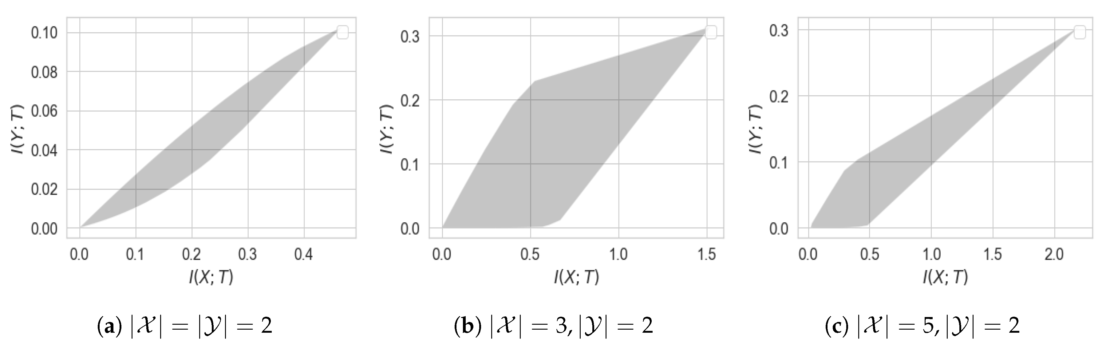
Figure 1 illustrates the set
for the simple case of binary
X and
Y.
While both
and
, their behavior in the neighborhood around zero might be completely different. As illustrated in
Figure 1,
for all
, whereas
for
for some
. When such
exists, we say perfect privacy occurs: there exists a variable
T satisfying
Y  X
X  T
T such that
while
; making
T a representation of
X having perfect privacy (i.e., no information leakage about
Y). A necessary and sufficient condition for the existence of such
T is given in [
21] (Lemma 10) and [
13] (Theorem 3), described next.
Theorem 2 (Perfect privacy). Let be given and be the set of vectors . Then there exists such that for if and only if vectors in are linearly independent.
In light of this theorem, we obtain that perfect privacy occurs if
. It also follows from the theorem that for binary
X, perfect privacy cannot occur (see
Figure 1a).
Theorem 1 enables us to derive a simple bounds for and . Specifically, the facts that is non-decreasing and is non-increasing immediately result in the the following linear bounds.
Theorem 3 (Linear lower bound)
. For , we have In light of this theorem, if
, then
, implying
for a deterministic function
g. Conversely, if
then
because for all
T forming the Markov relation
Y  g
g(
Y)
 T
T, we have
. On the other hand, we have
if and only if there exists a variable
satisfying
and thus the following double Markov relations
It can be verified (see [
79] (Problem 16.25)) that this double Markov condition is equivalent to the existence of a pair of functions
f and
g such that
and (
X,Y)
 f
f(
X)

. One special case of this setting, namely where
g is an identity function, has been recently studied in details in [
53] and will be reviewed in
Section 2.5. Theorem 3 also enables us to characterize the “worst” joint distribution
with respect to
and
. As demonstrated in the following lemma, if
is an erasure channel then
.
Lemma 1. Let be such that , , and for some . Then Let be such that , , and for some . Then
The bounds in Theorem 3 hold for all r and R in the interval . We can, however, improve them when r and R are sufficiently small. Let and denote the slope of and at zero, i.e., and .
Theorem 4. Given , we have This theorem provides the exact values of
and
and also simple bounds for them. While the exact expressions for
and
are usually difficult to compute, a simple plug-in estimator is proposed in [
80] for
. This estimator can be readily adapted to estimate
. Theorem 4 reveals a profound connection between
and the strong data processing inequality (SDPI) [
81]. More precisely, thanks to the pioneering work of Anantharam et al. [
82], it is known that the supremum of
over all
is equal the supremum of
over all
satisfying
Y  X
X  T
T and hence
specifies the strengthening of the data processing inequality of mutual information. This connection may open a new avenue for new theoretical results for
, especially when
X or
Y are continuous random variables. In particular, the recent non-multiplicative SDPI results [
27,
83] seem insightful for this purpose.
In many practical cases, we might have
n i.i.d. samples
of
. We now study how
behaves in
n. Let
and
. Due to the i.i.d. assumption, we have
. This can also be described by independently feeding
,
, to channel
producing
. The following theorem, demonstrated first in [
3] (Theorem 2.4), gives a formula for
in terms of
n.
This theorem demonstrates that an optimal channel
for i.i.d. samples
is obtained by the Kronecker product of an optimal channel
for
. This, however, may not hold in general for
, that is, we might have
, see [
13] (Proposition 1) for an example.
2.1. Gaussian and
In this section, we turn our attention to a special, yet important, case where
, where
and
is independent of
Y. This setting subsumes the popular case of jointly Gaussian
whose information bottleneck functional was computed in [
84] for the vector case (i.e.,
are jointly Gaussian random vectors).
Lemma 2. Let be n i.i.d. copies of and where are i.i.d samples of independent of Y. Then, we have It is worth noting that this result was concurrently proved in [
85]. The main technical tool in the proof of this lemma is a strong version of the entropy power inequality [
25] (Theorem 2) which holds even if
,
, and
are random vectors (as opposed to scalar). Thus, one can readily generalize Lemma 2 to the vector case. Note that the upper bound established in this lemma holds without any assumptions on
. This upper bound provides a significantly simpler proof for the well-known fact that for the jointly Gaussian
, the optimal channel
is Gaussian. This result was first proved in [
26] and used in [
84] to compute an expression of
for the Gaussian case.
Corollary 1. If are jointly Gaussian with correlation coefficient ρ, then we haveMoreover, the optimal channel is given by for where is the variance of Y. In Lemma 2, we assumed that
X is a Gaussian perturbation of
Y. However, in some practical scenarios, we might have
Y as a Gaussian perturbation of
X. For instance, let
X represent an image and
Y be a feature of the image that can be perfectly obtained from a noisy observation of
X. Then, the goal is to compress the image with a given compression rate while retaining maximal information about the feature. The following lemma, which is an immediate consequence of [
27] (Theorem 1), gives an upper bound for
in this case.
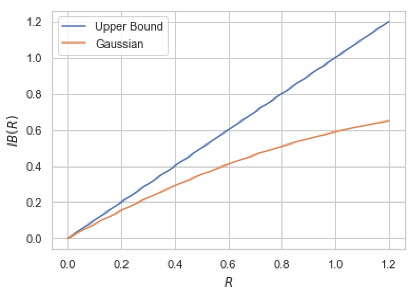
Lemma 3. Let be n i.i.d. copies of a random variable X satisfying and be the result of passing , , through a Gaussian channel , where and is independent of X. Then, we havewhere is the Gaussian complimentary CDF and for is the binary entropy function. Moreover, we have Note that that Lemma 3 holds for any arbitrary
X (provided that
) and hence (
9) bounds information bottleneck functionals for a wide family of
. However, the bound is loose in general for large values of
R. For instance, if
are jointly Gaussian (implying
for some
), then the right-hand side of (
9) does not reduce to (
8). To show this, we numerically compute the upper bound (
9) and compare it with the Gaussian information bottleneck (
8) in
Figure 2.
The privacy funnel functional is much less studied even for the simple case of jointly Gaussian. Solving the optimization in
over
without any assumptions is a difficult challenge. A natural assumption to make is that
is Gaussian for each
. This leads to the following variant of
where
and
is independent of
X. This formulation is tractable and can be computed in closed form for jointly Gaussian
as described in the following example.
Example 1. Let X and Y be jointly Gaussian with correlation coefficient ρ. First note that since mutual information is invariant to scaling, we may assume without loss of generality that both X and Y are zero mean and unit variance and hence we can write where is independent of Y. Consequently, we haveandIn order to ensure , we must have . Plugging this choice of σ into (13), we obtain This example indicates that for jointly Gaussian
, we have
if and only if
(thus perfect privacy does not occur) and the constraint
is satisfied by a unique
. These two properties in fact hold for all continuous variables
X and
Y with finite second moments as demonstrated in Lemma A1 in
Appendix A. We use these properties to derive a second-order approximation of
when
r is sufficiently small. For the following theorem, we use
to denote the variance of the random variable
U and
. We use
for short.
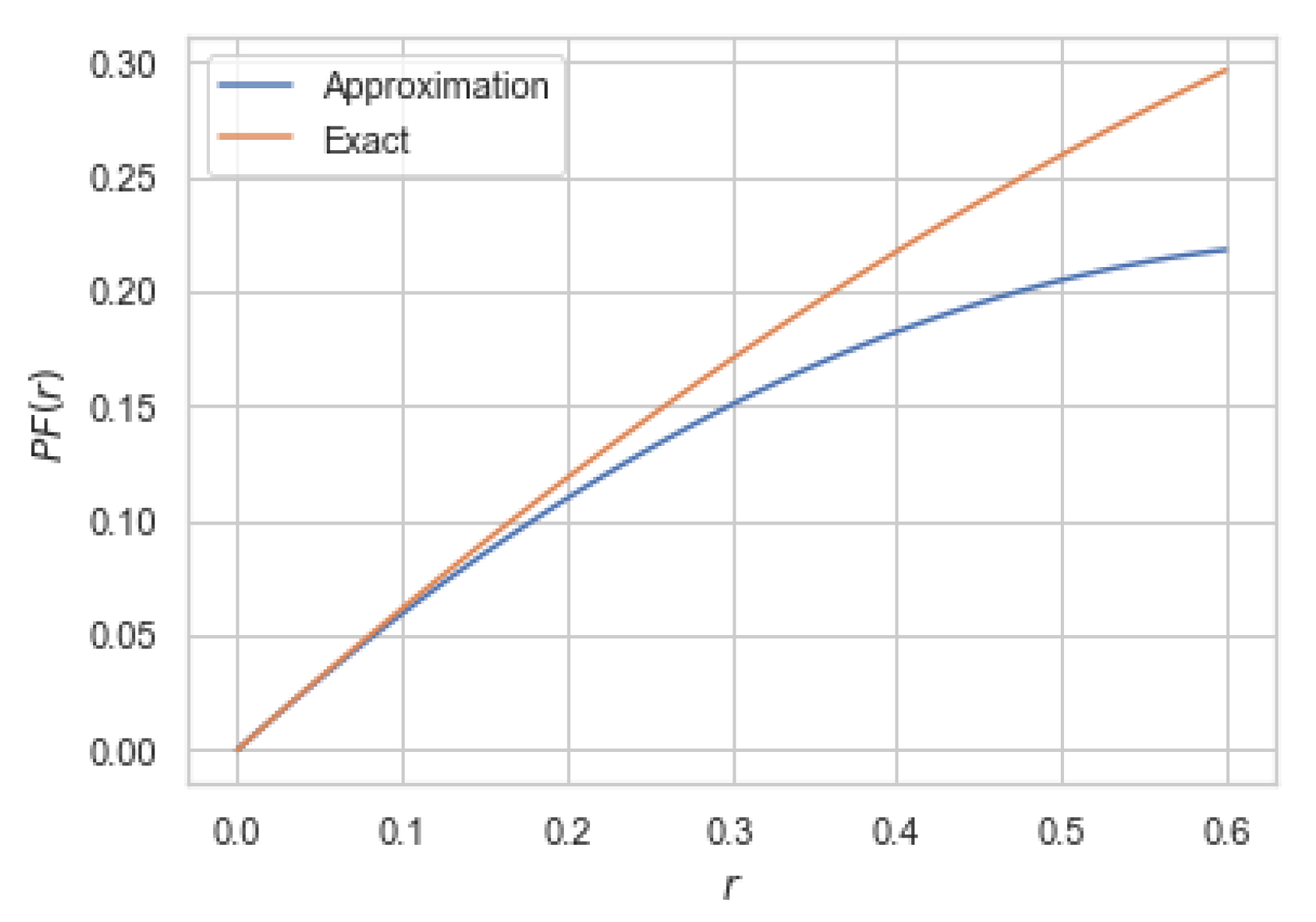
Theorem 6. For any pair of continuous random variables with finite second moments, we have as where and It is worth mentioning that the quantity
was first defined by Rényi [
28] as an asymmetric measure of correlation between
X and
Y. In fact, it can be shown that
where supremum is taken over all measurable functions
f and
denotes the correlation coefficient. As a simple illustration of Theorem 6, consider jointly Gaussian
X and
Y with correlation coefficient
for which
was computed in Example 1. In this case, it can be easily verified that
and
. Hence, for jointly Gaussian
with correlation coefficient
and unit variance, we have
. In
Figure 3, we compare the approximation given in Theorem 6 for this particular case.
2.2. Evaluation of and
The constrained optimization problems in the definitions of
and
are usually challenging to solve numerically due to the non-linearity in the constraints. In practice, however, both
and
are often approximated by their corresponding Lagrangian optimizations
and
where
is the Lagrangian multiplier that controls the tradeoff between compression and informativeness in for
and the privacy and informativeness in
. Notice that for the computation of
, we can assume, without loss of generality, that
since otherwise the maximizer of (
15) is trivial. It is worth noting that
and
in fact correspond to lines of slope
supporting
from above and below, thereby providing a new representation of
.
Let
be a pair of random variables with
for some
and
is the output of
when the input is
(i.e.,
). Define
This function, in general, is neither convex nor concave in
. For instance,
is concave and
is convex in
. The lower convex envelope of
is defined as the largest convex function smaller than
. Similarly, the upper concave envelope of
is defined as the smallest concave function larger than
. Let
and
denote the lower convex and upper concave envelopes of
, respectively. If
is convex at
, that is
, then
remains convex at
for all
because
where the last equality follows from the fact that
is convex. Hence, at
we have
Analogously, if
is concave at
, that is
, then
remains concave at
for all
.
Notice that, according to (
15) and (
16), we can write
and
In light of the above arguments, we can write
for all
where
is the smallest
such that
touches
. Similarly,
for all
where
is the largest
such that
touches
. In the following theorem, we show that
and
are given by the values of
and
, respectively, given in Theorem 4. A similar formulae
and
were given in [
86].
Kim et al. [
80] have recently proposed an efficient algorithm to estimate
from samples of
involving a simple optimization problem. This algorithm can be readily adapted for estimating
. Proposition 1 implies that in optimizing the Lagrangians (
17) and (
18), we can restrict the Lagrange multiplier
, that is
and
Remark 1. As demonstrated by Kolchinsky et al. [53], the boundary points 0 and are required for the computation of . In fact, when Y is a deterministic function of X, then only
and are required to compute the and other values of β are vacuous. The same argument can also be used to justify the inclusion of in computing . Note also that since becomes convex for , computing becomes trivial for such values of β. Remark 2. Observe that the lower convex envelope of any function f can be obtained by taking Legendre-Fenchel transformation (aka. convex conjugate) twice. Hence, one can use the existing linear-time algorithms for approximating Legendre-Fenchel transformation (e.g., [87,88]) for approximating . Once
and
are computed, we can derive
and
via standard results in optimization (see [
3] (Section IV) for more details):
and
Following the convex analysis approach outlined by Witsenhausen and Wyner [
3],
and
can be directly computed from
and
by observing the following. Suppose for some
,
(resp.
) at
is obtained by a convex combination of points
,
for some
in
, integer
, and weights
(with
). Then
, and
with properties
and
attains the minimum (resp. maximum) of
. Hence,
is a point on the upper (resp. lower) boundary of
; implying that
for
(resp.
for
). If for some
,
at
coincides with
, then this corresponds to
. The same holds for
. Thus, all the information about the functional
(resp.
) is contained in the subset of the domain of
(resp.
) over which it differs from
. We will revisit and generalize this approach later in
Section 3.
We can now instantiate this for the binary symmetric case. Suppose
X and
Y are binary variables and
is binary symmetric channel with crossover probability
, denoted by
and defined as
for some
. To describe the result in a compact fashion, we introduce the following notation: we let
denote the binary entropy function, i.e.,
. Since this function is strictly increasing
, its inverse exists and is denoted by
. Moreover,
for
.
Lemma 4 (Mr. and Mrs. Gerber’s Lemma)
. For for and for , we haveandwhere , , and . The result in (
24) was proved by Wyner and Ziv [
2] and is widely known as Mrs. Gerber’s Lemma in information theory. Due to the similarity, we refer to (
25) as Mr. Gerber’s Lemma. As described above, to prove (
24) and (
25) it suffices to derive the convex and concave envelopes of the mapping
given by
where
is the output distribution of
when the input distribution is
for some
. It can be verified that
. This function is depicted in
Figure 4 depending of the values of
.
2.3. Operational Meaning of and
In this section, we illustrate several information-theoretic settings which shed light on the operational interpretation of both
and
. The operational interpretation of
has recently been extensively studied in information-theoretic settings in [
29,
30]. In particular, it was shown that
specifies the rate-distortion region of noisy source coding problem [
19,
89] under the logarithmic loss as the distortion measure and also the rate region of the lossless source coding with side information at the decoder [
90]. Here, we state the former setting (as it will be useful for our subsequent analysis of cardinality bound) and also provide a new information-theoretic setting in which
appears as the solution. Then, we describe another setting, the so-called dependence dilution, whose achievable rate region has an extreme point specified by
. This in fact delineate an important difference between
and
: while
describes the entire rate-region of an information-theoretic setup,
specifies only a corner point of a rate region. Other information-theoretic settings related to
and
include CEO problem [
91] and source coding for the Gray-Wyner network [
92].
2.3.1. Noisy Source Coding
Suppose Alice has access only to a noisy version
X of a source of interest
Y. She wishes to transmit a rate-constrained description from her observation (i.e.,
X) to Bob such that he can recover
Y with small average distortion. More precisely, let
be
n i.i.d. samples of
. Alice encodes her observation
through an encoder
and sends
to Bob. Upon receiving
, Bob reconstructs a “soft” estimate of
via a decoder
where
. That is, the reproduction sequence
consists of
n probability measures on
. For any source and reproduction sequences
and
, respectively, the distortion is defined as
where
We say that a pair of rate-distortion
is achievable if there exists a pair
of encoder and decoder such that
The noisy rate-distortion function
for a given
, is defined as the minimum rate
such that
is an achievable rate-distortion pair. This problem arises naturally in many data analytic problems. Some examples include feature selection of a high-dimensional dataset, clustering, and matrix completion. This problem was first studied by Dobrushin and Tsybakov [
19], who showed that
is analogous to the classical rate-distortion function
It can be easily verified that
and hence (after relabeling
as
T)
where
, which is equal to
defined in (
4). For more details in connection between noisy source coding and
, the reader is referred to [
29,
30,
91,
93]. Notice that one can study an essentially identical problem where the distortion constraint (
28) is replaced by
This problem is addressed in [
94] for discrete alphabets
and
and extended recently in [
95] for any general alphabets.
2.3.2. Test against Independence with Communication Constraint
As mentioned earlier, the connection between
and noisy source coding, described above, was known and studied in [
29,
30]. Here, we provide a new information-theoretic setting which provides yet another operational meaning for
. Given
n i.i.d. samples
from joint distribution
Q, we wish to test whether
are independent of
, that is,
Q is a product distribution. This task is formulated by the following hypothesis test:
for a given joint distribution
with marginals
and
. Ahlswede and Csiszár [
20] investigated this problem under a communication constraint: While
Y observations (i.e.,
) are available, the
X observations need to be compressed at rate
R, that is, instead of
, only
is present where
satisfies
For the type I error probability not exceeding a fixed
, Ahlswede and Csiszár [
20] derived the smallest possible type 2 error probability, defined as
The following gives the asymptotic expression of
for every
. For the proof, refer to [
20] (Theorem 3).
Theorem 7 ([
20])
. For every and , we have In light of this theorem,
specifies the exponential rate at which the type II error probability of the hypothesis test (
31) decays as the number of samples increases.
2.3.3. Dependence Dilution
Inspired by the problems of information amplification [
96] and state masking [
97], Asoodeh et al. [
21] proposed the dependence dilution setup as follows. Consider a source sequences
of
n i.i.d. copies of
. Alice observes the source
and wishes to encode it via the encoder
for some
. The goal is to ensure that any user observing
can construct a list, of fixed size, of sequences in
that contains likely candidates of the actual sequence
while revealing negligible information about a correlated source
. To formulate this goal, consider the decoder
where
denotes the power set of
. A
dependence dilution triple is said to be achievable if, for any
, there exists a pair of encoder and decoder
such that for sufficiently large
n
having fixed size
where
and simultaneously
Notice that without side information
J, the decoder can only construct a list of size
which contains
with probability close to one. However, after
J is observed and the list
is formed, the decoder’s list size can be reduced to
and thus reducing the uncertainty about
by
. This observation can be formalized to show (see [
96] for details) that the constraint (
32) is equivalent to
which lower bounds the amount of information
J carries about
. Built on this equivalent formulation, Asoodeh et al. [
21] (Corollary 15) derived a necessary condition for the achievable dependence dilution triple.
Theorem 8 ([
21])
. Any achievable dependence dilution triple satisfiesfor some auxiliary random variable T satisfying Y  X
X  T and taking values.
 According to this theorem, specifies the best privacy performance of the dependence dilution setup for the maximum amplification rate . While this informs the operational interpretation of , Theorem 8 only provides an outer bound for the set of achievable dependence dilution triple . It is, however, not clear that characterizes the rate region of an information-theoretic setup.
The fact that fully characterizes the rate-region of an source coding setup has an important consequence: the cardinality of the auxiliary random variable T in can be improved to instead of .
2.4. Cardinality Bound
Recall that in the definition of
in (
4), no assumption was imposed on the auxiliary random variable
T. A straightforward application of Carathéodory-Fenchel-Eggleston theorem (see e.g., [
98] (Section III) or [
79] (Lemma 15.4)) reveals that
is attained for
T taking values in a set
with cardinality
. Here, we improve this bound and show
is sufficient.
Theorem 9. For any joint distribution and , information bottleneck is achieved by T taking at most values.
The proof of this theorem hinges on the operational characterization of
as the lower boundary of the rate-distortion region of noisy source coding problem discussed in
Section 2.3. Specifically, we first show that the extreme points of this region is achieved by
T taking
values. We then make use of a property of the noisy source coding problem (namely, time-sharing) to argue that all points of this region (including the boundary points) can be attained by such
T. It must be mentioned that this result was already claimed by Harremoës and Tishby in [
99] without proof.
In many practical scenarios, feature
X has a large alphabet. Hence, the bound
, albeit optimal, still can make the information bottleneck function computationally intractable over large alphabets. However, label
Y usually has a significantly smaller alphabet. While it is in general impossible to have a cardinality bound for
T in terms of
, one can consider approximating
assuming
T takes
N values. The following result, recently proved by Hirche and Winter [
100], is in this spirit.
Theorem 10 ([
100])
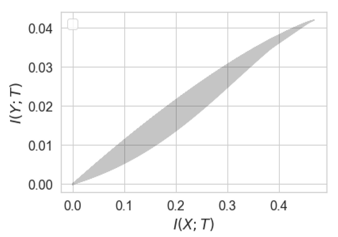
. For any , we havewhere and denotes the information bottleneck functional (4) with the additional constraint that . Recall that, unlike
, the graph of
characterizes the rate region of a Shannon-theoretic coding problem (as illustrated in
Section 2.3), and hence any boundary points can be constructed via time-sharing of extreme points of the rate region. This lack of operational characterization of
translates into a worse cardinality bound than that of
. In fact, for
the cardinality bound
cannot be improved in general. To demonstrate this, we numerically solve the optimization in
assuming that
when both
X and
Y are binary. As illustrated in
Figure 5, this optimization does not lead to a convex function, and hence, cannot be equal to
.
2.5. Deterministic Information Bottleneck
As mentioned earlier,
formalizes an information-theoretic approach to clustering high-dimensional feature
X into cluster labels
T that preserve as much information about the label
Y as possible. The clustering label is assigned by the soft operator
that solves the
formulation (
4) according to the rule:
is likely assigned label
if
is small where
. That is, clustering is assigned based on the similarity of conditional distributions. As in many practical scenarios, a hard clustering operator is preferred, Strouse and Schwab [
31] suggested the following variant of
, termed as deterministic information bottleneck
where the maximization is taken over all deterministic functions
f whose range is a finite set
. Similarly, one can define
One way to ensure that
for a deterministic function
f is to restrict the cardinality of the range of
f: if
then
is necessarily smaller than
R. Using this insight, we derive a lower for
in the following lemma.
Lemma 5. For any given , we haveand Note that both
R and
r are smaller than
and thus the multiplicative factors of
in the lemma are smaller than one. In light of this lemma, we can obtain
and
In most of practical setups,
might be very large, making the above lower bound for
vacuous. In the following lemma, we partially address this issue by deriving a bound independent of
when
Y is binary.
Lemma 6. Let be a joint distribution of arbitrary X and binary for some . Then, for any we havewhere . 3. Family of Bottleneck Problems
In this section, we introduce a family of bottleneck problems by extending
and
to a large family of statistical measures. Similar to
and
, these bottleneck problems are defined in terms of boundaries of a two-dimensional convex set induced by a joint distribution
. Recall that
and
are the upper and lower boundary of the set
defined in (
6) and expressed here again for convenience
Since
is given,
and
are fixed. Thus, in characterizing
it is sufficient to consider only
and
. To generalize
and
, we must therefore generalize
and
.
Given a joint distribution
and two non-negative real-valued functions
and
, we define
and
When
and
, we interchangeably write
for
and
for
.
These definitions provide natural generalizations for Shannon’s entropy and mutual information. Moreover, as we discuss later in
Section 3.2 and
Section 3.3, it also can be specialized to represent a large family of popular information-theoretic and statistical measures. Examples include information and estimation theoretic quantities such as Arimoto’s conditional entropy of order
for
, probability of correctly guessing for
, maximal correlation for binary case, and
f-information for
given by
f-divergence. We are able to generate a family of bottleneck problems using different instantiations of
and
in place of mutual information in
and
. As we argue later, these problems better capture the essence of “informativeness” and “privacy”; thus providing analytical and interpretable guarantees similar in spirit to
and
.
Computing these bottleneck problems in general boils down to the following optimization problems
and
Consider the set
Note that if both
and
are continuous (with respect to the total variation distance), then
is compact. Moreover, it can be easily verified that
is convex. Hence, its upper and lower boundaries are well-defined and are characterized by the graphs of
and
, respectively. As mentioned earlier, these functional are instrumental for computing the general bottleneck problem later. Hence, before we delve into the examples of bottleneck problems, we extend the approach given in
Section 2.2 to compute
and
.
3.1. Evaluation of and
Analogous to
Section 2.2, we first introduce the Lagrangians of
and
as
and
where
is the Lagrange multiplier, respectively. Let
be a pair of random variable with
and
is the result of passing
through the channel
. Letting
we obtain that
recalling that
and
are the upper concave and lower convex envelop operators. Once we compute
and
for all
, we can use the standard results in optimizations theory (similar to (
21) and (
22)) to recover
and
. However, we can instead extend the approach Witsenhausen and Wyner [
3] described in
Section 2.2. Suppose for some
,
(resp.
) at
is obtained by a convex combination of points
,
for some
in
, integer
, and weights
(with
). Then
, and
with properties
and
attains the maximum (resp. minimum) of
, implying that
is a point on the upper (resp. lower) boundary of
. Consequently, such
satisfies
for
(resp.
for
). The algorithm to compute
and
is then summarized in the following three steps:
Construct the functional for and and all and .
Compute and evaluated at .
If for distributions in for some , we have or for some satisfying , then then , and give the optimal in and , respectively.
We will apply this approach to analytically compute and (and the corresponding bottleneck problems) for binary cases in the following sections.
3.2. Guessing Bottleneck Problems
Let
be given with marginals
and
and the corresponding channel
. Let also
be an arbitrary distribution on
and
be the output distribution of
when fed with
. Any channel
, together with the Markov structure
Y  X
X  T
T, generates unique
and
. We need the following basic definition from statistics.
Definition 1. Let U be a discrete and V be an arbitrary random variables supported on and with , respectively. Then the probability of correctly guessing U and the probability of correctly guessing U given V are given byandMoreover, the multiplicative gain of the observation V in guessing U is defined as (the reason for ∞ in the notation becomes clear later) As the names suggest, and characterize the optimal efficiency of guessing U with or without the observation V, respectively. Intuitively, quantifies how useful the observation V is in estimating U: If it is small, then it means it is nearly as hard for an adversary observing V to guess U as it is without V. This observation motivates the use of as a measure of privacy in lieu of in .
It is worth noting that
is not symmetric in general, i.e.,
. Since observing
T can only improve, we have
; thus
. However,
does not necessarily imply independent of
Y and
T; instead, it means
T is useless in estimating
Y. As an example, consider
and
and
with
. Then
and
Thus, if
, then
. This then implies that
whereas
Y and
T are clearly dependent; i.e.,
. While in general
and
are not related, it can be shown that
if
Y is uniform (see [
65] (Proposition 1)). Hence, only with this uniformity assumption,
implies the independence.
Consider
and
. Clearly, we have
. Note that
thus both measures
and
are special cases of the models described in the previous section. In particular, we can define the corresponding
and
. We will see later that
and
correspond to Arimoto’s mutual information of orders 1 and
∞, respectively. Define
This bottleneck functional formulated an interpretable guarantee:
Recall that the functional
aims at extracting maximum information of
X while protecting privacy with respect to
Y. Measuring the privacy in terms of
, this objective can be better formulated by
with the interpretable privacy guarantee:
Notice that the variable
T in the formulations of
and
takes values in a set
of arbitrary cardinality. However, a straightforward application of the Carathéodory-Fenchel-Eggleston theorem (see e.g., [
79] (Lemma 15.4)) reveals that the cardinality of
can be restricted to
without loss of generality. In the following lemma, we prove more basic properties of
and
.
Lemma 7. For any with Y supported on a finite set , we have
.
for any and for .
is strictly increasing and concave on the range .
is strictly increasing, and convex on the range .
The proof follows the same lines as Theorem 1 and hence omitted. Lemma 7 in particular implies that inequalities
and
in the definition of
and
can be replaced by
and
, respectively. It can be verified that
satisfies the data-processing inequality, i.e.,
for the Markov chain
Y  X
X  T
T. Hence, both
and
must be smaller than
. The properties listed in Lemma 7 enable us to derive a slightly tighter upper bound for
as demonstrated in the following.
Lemma 8. For any with Y supported on a finite set , we haveand The proof of this lemma (and any other results in this section) is given in
Appendix B. This lemma shows that the gap between
and
when
R is sufficiently close to
behaves like
Thus,
approaches
as
at least linearly.
In the following theorem, we apply the technique delineated in
Section 3.1 to derive closed form expressions for
and
for the binary symmetric case, thereby establishing similar results as Mr and Mrs. Gerber’s Lemma.
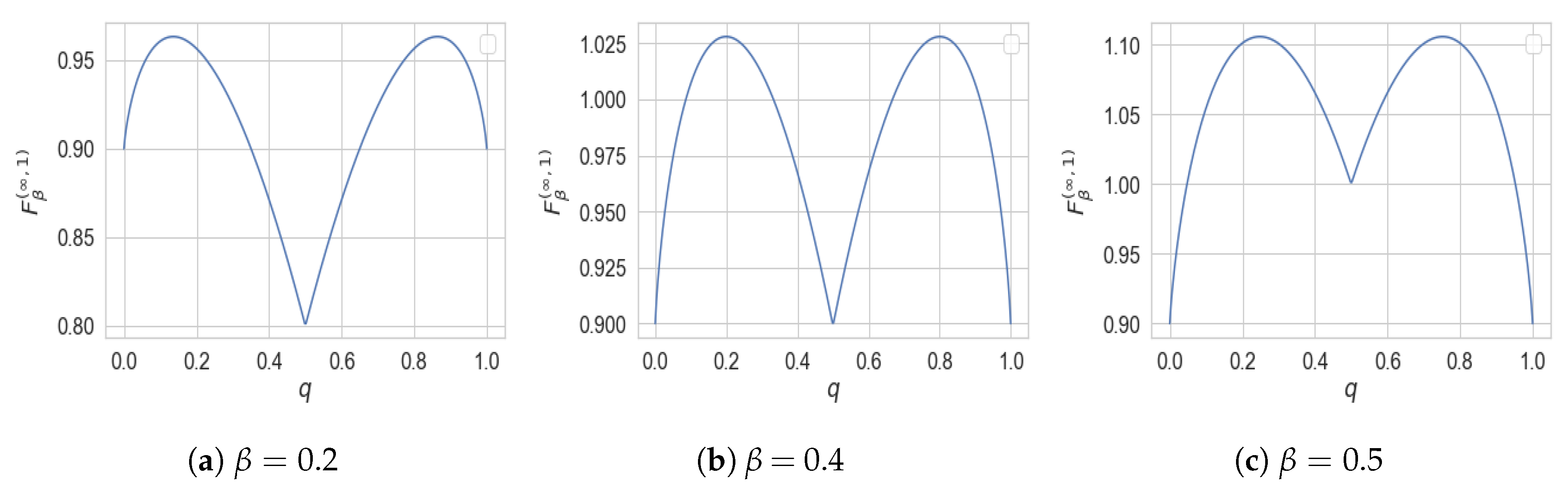
Theorem 11. For and with , we haveandwhere . As described in
Section 3.1, to compute
and
it suffices to derive the convex and concave envelopes of the mapping
where
and
is the result of passing
through
, i.e.,
. In this case,
and
can be expressed as
This function is depicted in
Figure 6.
The detailed derivation of convex and concave envelope of
is given in
Appendix B. The proof of this theorem also reveals the following intuitive statements. If
and
, then among all random variables
T satisfying
Y  X
X  T
T and
, the minimum
is given by
. Notice that, without any information constraint (i.e.,
),
. Perhaps surprisingly, this shows that the mutual information constraint has a linear effect on the privacy of
Y. Similarly, to prove (
51), we show that among all
R-bit representations
T of
X, the best achievable accuracy
is given by
. This can be proved by combining Mrs. Gerber’s Lemma (cf. Lemma 4) and Fano’s inequality as follows. For all
T such that
, the minimum of
is given by
. Since by Fano’s inequality,
, we obtain
which leads to the same result as above. Nevertheless, in
Appendix B we give another proof based on the discussion of
Section 3.1.
3.3. Arimoto Bottleneck Problems
The bottleneck framework proposed in the last section benefited from interpretable guarantees brought forth by the quantity . In this section, we define a parametric family of statistical quantities, the so-called Arimoto’s mutual information, which includes both Shannon’s mutual information and as extreme cases.
Definition 2 ([
22])
. Let and be two random variables supported over finite sets and , respectively. Their Arimoto’s mutual information of order is defined aswhereis the Rényi entropy of order α andis the Arimoto’s conditional entropy of order α. By continuous extension, one can define
for
and
as
and
, respectively. That is,
Arimoto’s mutual information was first introduced by Arimoto [
22] and then later revisited by Liese and Vajda in [
101] and more recently by Verdú in [
102]. More in-depth analysis and properties of
can be found in [
103]. It is shown in [
71] (Lemma 1) that
for
quantifies the minimum loss in recovering
U given
V where the loss is measured in terms of the so-called
-loss. This loss function reduces to logarithmic loss (
27) and
for
and
, respectively. This sheds light on the utility and/or privacy guarantee promised by a constraint on Arimoto’s mutual information. It is now natural to use
for defining a family of bottleneck problems.
Definition 3. Given a pair of random variables over finite sets and and , we define and asand Of course,
and
. It is known that Arimoto’s mutual information satisfies the data-processing inequality [
103] (Corollary 1), i.e.,
for the Markov chain
Y  X
X  T
T. On the other hand,
. Thus, both
and
equal
for
. Note also that
where
(see (
39)) corresponding to the function
. Consequently,
and
are characterized by the lower and upper boundary of
, defined in (
37), with respect to
and
. Specifically, we have
where
, and
where
and
and
. This paves the way to apply the technique described in
Section 2.2 to compute
and
. Doing so requires the upper concave and lower convex envelope of the mapping
for some
, where
. In the following theorem, we drive these envelopes and give closed form expressions for
and
for a special case where
.
Theorem 12. Let and with . We have for where for and solvesMoreover,where and solves By letting
, this theorem indicates that for
X and
Y connected through
and all variables
T forming
Y  X
X  T
T, we have
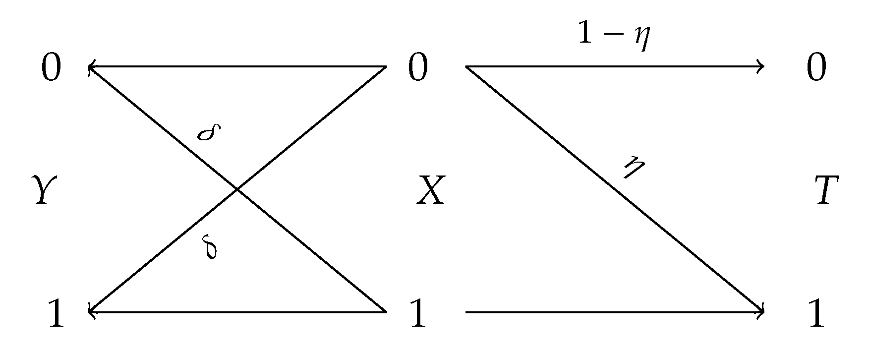
which can be shown to be achieved
generated by the following channel (see
Figure 7)
Note that, by assumption,
, and hence the event
is less likely than
. Therefore, (
61) demonstrates that to ensure correct recoverability of
X with probability at lest
, the most private approach (with respect to
Y) is to obfuscate the higher-likely event
with probability
. As demonstrated in (
61) the optimal privacy guarantee is linear in the utility parameter in the binary symmetric case. This is in fact a special case of the larger result recently proved in [
65] (Theorem 1): the infimum of
over all variables
T such that
is piece-wise linear in
, on equivalently, the mapping
is piece-wise linear.
Computing analytically for every seems to be challenging, however, the following lemma provides bounds for and in terms of and , respectively.
Lemma 9. For any pair of random variables over finite alphabets and , we haveandwhere and . The previous lemma can be directly applied to derive upper and lower bounds for and given and .
3.4. f-Bottleneck Problems
In this section, we describe another instantiation of the general framework introduced in terms of functions and that enjoys interpretable estimation-theoretic guarantee.
Definition 4. Let be a convex function with . Furthermore, let U and V be two real-valued random variables supported over and , respectively. Their f-information is defined bywhere is the f-divergence [104] between distributions and defined as Due to convexity of
f, we have
and hence
f-information is always non-negative. If, furthermore,
f is strictly convex at 1, then equality holds if and only
. Csiszár introduced
f-divergence in [
104] and applied it to several problems in statistics and information theory. More recent developments about the properties of
f-divergence and
f-information can be found in [
23] and the references therein. Any convex function
f with the property
results in an
f-information. Popular examples include
corresponding to Shannon’s mutual information,
corresponding to
T-information [
83], and also
corresponding to
-information [
69] for. It is worth mentioning that if we allow
to be in
in Definition 2 (similar to [
101]), then the resulting Arimoto’s mutual information can be shown to be an
f-information in the binary case for a certain function
f, see [
101] (Theorem 8).
Let
be given with marginals
and
. Consider functions
and
on
and
defined as
Given a conditional distribution
, it is easy to verify that
and
. This in turn implies that
f-information can be utilized in (
40) and (
41) to define general bottleneck: Let
and
be two convex functions satisfying
. Then we define
and
In light of the discussion in
Section 3.1, the optimization problems in
and
can be analytically solved by determining the upper concave and lower convex envelope of the mapping
where
is the Lagrange multiplier and
.
Consider the function
with
. The corresponding
f-divergence is sometimes called Hellinger divergence of order
, see e.g., [
105]. Note that Hellinger divergence of order 2 reduces to
-divergence. Calmon et al. [
68] and Asoodeh et al. [
67] showed that if
for some
, then the minimum mean-squared error (MMSE) of reconstructing any zero-mean unit-variance function of
Y given
T is lower bounded by
, i.e., no function of
Y can be reconstructed with small MMSE given an observation of
T. This result serves a natural justification for
as an operational measure of both privacy and utility in a bottleneck problem.
Unfortunately, our approach described in
Section 3.1 cannot be used to compute
or
in the binary symmetric case. The difficulty lies in the fact that the function
, defined in (
66), for the binary symmetric case is either convex or concave on its entire domain depending on the value of
. Nevertheless, one can consider Hellinger divergence of order
with
and then apply our approach to compute
or
. Since
(see [
106] (Corollary 5.6)), one can justify
as a measure of privacy and utility in a similar way as
.
We end this section by a remark about estimating the measures studied in this section. While we consider information-theoretic regime where the underlying distribution
is known, in practice only samples
are given. Consequently, the de facto guarantees of bottleneck problems might be considerably different from those shown in this work. It is therefore essential to asses the guarantees of bottleneck problems when accessing only samples. To do so, one must derive bounds on the discrepancy between
,
, and
computed on the empirical distribution and the true (unknown) distribution. These bounds can then be used to shed light on the de facto guarantee of the bottleneck problems. Relying on [
34] (Theorem 1), one can obtain that the gaps between the measures
,
, and
computed on empirical distributions and the true one scale as
where
n is the number of samples. This is in contrast with mutual information for which the similar upper bound scales as
as shown in [
33]. Therefore, the above measures appear to be easier to estimate than mutual information.
4. Summary and Concluding Remarks
Following the recent surge in the use of information bottleneck (
) and privacy funnel (
) in developing and analyzing machine learning models, we investigated the functional properties of these two optimization problems. Specifically, we showed that
and
correspond to the upper and lower boundary of a two-dimensional convex set
Y  X
X  T
T} where
represents the observable data
X and target feature
Y and the auxiliary random variable
T varies over all possible choices satisfying the Markov relation
Y  X
X  T
T. This unifying perspective on
and
allowed us to adapt the classical technique of Witsenhausen and Wyner [
3] devised for computing
to be applicable for
as well. We illustrated this by deriving a closed form expression for
in the binary case—a result reminiscent of the Mrs. Gerber’s Lemma [
2] in information theory literature. We then showed that both
and
are closely related to several information-theoretic coding problems such as noisy random coding, hypothesis testing against independence, and dependence dilution. While these connections were partially known in previous work (see e.g., [
29,
30]), we show that they lead to an improvement on the cardinality of
T for computing
. We then turned our attention to the continuous setting where
X and
Y are continuous random variables. Solving the optimization problems in
and
in this case without any further assumptions seems a difficult challenge in general and leads to theoretical results only when
is jointly Gaussian. Invoking recent results on the entropy power inequality [
25] and strong data processing inequality [
27], we obtained tight bounds on
in two different cases: (1) when
Y is a Gaussian perturbation of
X and (2) when
X is a Gaussian perturbation of
Y. We also utilized the celebrated I-MMSE relationship [
107] to derive a second-order approximation of
when
T is considered to be a Gaussian perturbation of
X.
In the second part of the paper, we argue that the choice of (Shannon’s) mutual information in both
and
does not seem to carry specific operational significance. It does, however, have a desirable practical consequence: it leads to self-consistent equations [
1] that can be solved iteratively (without any guarantee to convergence though). In fact, this property is unique to mutual information among other existing information measures [
99]. Nevertheless, we argued that other information measures might lead to better interpretable guarantee for both
and
. For instance, statistical accuracy in
and privacy leakage in
can be shown to be precisely characterized by probability of correctly guessing (aka Bayes risk) or minimum mean-squared error (MMSE). Following this observation, we introduced a large family of optimization problems, which we call bottleneck problems, by replacing mutual information in
and
with Arimoto’s mutual information [
22] or
f-information [
23]. Invoking results from [
33,
34], we also demonstrated that these information measures are in general easier to estimate from data than mutual information. Similar to
and
, the bottleneck problems were shown to be fully characterized by boundaries of a two-dimensional convex set parameterized by two real-valued non-negative functions
and
. This perspective enabled us to generalize the technique used to compute
and
for evaluating bottleneck problems. Applying this technique to the binary case, we derived closed form expressions for several bottleneck problems.


 X
X 


