A Review of the Classical Canonical Ensemble Treatment of Newton’s Gravitation

Abstract

It is common lore that the canonical gravitational partition function $\mathcal{Z}$ associated with the classical Boltzmann-Gibbs (BG) exponential distribution cannot be built up because of mathematical pitfalls. The integral needed for writing up $\mathcal{Z}$ diverges. We review here how to avoid this pitfall and obtain a (classical) statistical mechanics of Newton’s gravitation. This is done using (1) the analytical extension treatment obtained of Gradshteyn and Rizhik and (2) the well known dimensional regularization technique.

1. Introduction

Common lore asserts that, in dealing with gravity, the classical Boltzmann-Gibbs (BG) probability distribution is unable to produce finite results. Why? Because the pertinent partition function $\mathcal{Z}$ diverges in any $\nu$ dimensional space [1,2,3,4,5]. If one calls m and M the masses involved, $\nu$ the number of space-dimensions, G the gravitation constant, $\beta$ the inverse temperature, and x-p the phase-space coordinates, one has

$${\mathcal{Z}}_{\nu }=\underset{R}{\int }{e}^{-\beta \left(\frac{p^2}{2m}-\frac{GmM}{r}\right)}{d}^{\nu }x{d}^{\nu }p,$$

(1)

involving a positive exponential. However, common lore is not able to envision the possibility of taking care of such divergences via dimensional regularization. Note that Z is not an observable, what matters is the convergence of physical expectations values one builds with it.

Dimensional regularization (DR) [6,7,8,9,10] can be regarded as a very important advance in theoretical physics. Actually DR is now well over 40 years old. It is appealed to in variegated branches of physics (see, as examples, the 54 references cited in Reference [11]).

The contents of Reference [12] will be reviewed here. There, for first time ever, a finite gravitational $\mathcal{Z}$ was computed for Boltzmann entropy using a generalization of the DR technique [12]. The feat was repeated, this time for Tsallis statistics in Reference [11]. We wish here to review these results in a rather accessible manner.

The present work intends to review the conjoining of gravitation plus DR to produce a finite thermo-statistics. The statistical mechanics of gravitation needs revisiting, we feel, because it has not yet percolated into the Statistical Mechanics community. Thus, in this effort we review the main points of how to overcome the above-mentioned technical problem of divergences by judicious use of an appropriate combination of (i) dimensional regularization and (ii) analytical extension. We remark that we deal only with two-body gravitational interactions. The more general N-bodies gravitational problem has not yet been solved. Indeed, it constitutes a frontier problem in Celestial Mechanics. We are not concerned with the general problem here.

Note also that, as is well known, at the quantum field theory level, the usual dimensional regularization cannot cope with the gravitational field (because it is non-renormalizable). Our present elaborations are of a quite different kind, though, because we will deal with Newton’s classical gravity. We apply our generalization of dimensional regularization [10], with which it is possible treat non-renormalizable theories.

2. Illustrating the Mechanism of Dimensional Regularization (DR) in a Simple Context

Let us discuss DR in a simple environment, accepting its justification as reported in Reference [10], that in turn generalizes References [6,7,8].

A first example is obtained using Tsallis’ q-entropy $S_T$[13] ($q\in \mathcal{R}$). We look at a harmonic oscillator (HO) whose Hamiltonian reads simply

$$H=P^2+Q^2.$$

(2)

Now, for this system the q-probability distribution $P_t$ can be cast as [13]

$$P_t={\mathcal{Z}}^{-1}{[1+(1-q)\beta (P^2+Q^2)]}^{\frac{1}{q-1}}.$$

(3)

In turn, the $q-$entropy $S_T$ becomes

$$S_T=\frac{1-\underset{R}{\int }{P}_t^{q}d\mu }{q-1}.$$

(4)

We concentrate our efforts on the partition function $\mathcal{Z}$ for the HO in three dimensions. The first DR idea is to re-write $\mathcal{Z}$ in $\nu$ dimensions, not in 3.

$$\mathcal{Z}=\int {[1+(1-q)\beta (P^2+Q^2)]}^{\frac{1}{q-1}}{d}^{\nu }p{d}^{\nu }q,$$

(5)

where $P^2=p_1^2+p_2^2+\cdots p_{\nu }^2$ and $Q^2=q_1^2+q_2^2+\cdots q_{\nu }^2$. In dealing with these kind of integrals one employs hyper-spherical coordinates and has

$$\mathcal{Z}=\frac{2{\pi }^{\nu }}{\Gamma \left(\nu \right)}\underset{0}{\overset{\infty }{\int }}{s}^{2\nu -1}{[1+(1-q)\beta s^2]}^{\frac{1}{q-1}}ds,$$

(6)

where $s^2=P^2+Q^2$. With the replacement $s^2=x$ one finds

$$\mathcal{Z}=\frac{{\pi }^{\nu }}{\Gamma \left(\nu \right)}\underset{0}{\overset{\infty }{\int }}\frac{x^{\nu -1}}{{[1+(1-q)\beta x]}^{\frac{1}{1-q}}}dx.$$

(7)

This integral can be looked up in Reference [14].

$$\frac{{\pi }^{\nu }}{\Gamma \left(\nu \right)}\underset{0}{\overset{\infty }{\int }}\frac{x^{\mu -1}}{{(1+\gamma x)}^v}dx={\gamma }^{-\mu }B(\mu ,v-\mu ),$$

(8)

where $B(\mu ,v-\mu )$ is the celebrated Euler Beta function. Matching (7) to (8) one discovers that $\mu =\nu$, $v=\frac{1}{1-q}$, $\gamma =(1-q)\beta$. Accordingly,

$$\mathcal{Z}=\frac{{\pi }^{\nu }}{\Gamma \left(\nu \right)}{\left[\beta (1-q)\right]}^{-\nu }B\left(\nu ,\frac{1}{1-q}-\nu \right),$$

(9)

where

$$B\left(\nu ,\frac{1}{1-q}-\nu \right)=\frac{\Gamma \left(\nu \right)\Gamma \left(\frac{1}{1-q}-\nu \right)}{\Gamma \left(\frac{1}{1-q}\right)}.$$

(10)

Note that $\Gamma \left(z\right)$ stands for the well known Gamma function of Euler. It displays poles at $z=0,-1,-2,-3,\dots .$ (all negative integer numbers and also zero). (10) entails

$$\mathcal{Z}={\left[\frac{\pi }{\beta (1-q)}\right]}^{\nu }\frac{\Gamma \left(\frac{1}{1-q}-\nu \right)}{\Gamma \left(\frac{1}{1-q}\right)}.$$

(11)

Following now Reference [11], we set $q=\frac{2}{3}$ in (11). Since $\Gamma \left(3\right)=2$, we are led to

$$\mathcal{Z}=\frac{1}{2}{\left(\frac{3\pi }{\beta }\right)}^{\nu }\Gamma \left(3-\nu \right).$$

(12)

One notes that for $\nu =3$, $\mathcal{Z}$ does diverge. We have generalized Bollini-Giambiagi’s DR approach by performing a Laurent-expansion (LE) of $\mathcal{Z}$ around $\nu =3$ and selecting after this what one regards as the physical $\mathcal{Z}$-result, i.e., the $\nu -3$-independent term of the LE. We justify this procedure in Appendix A. We now proceed with the LE by defining

$$f\left(\nu \right)={\left(\frac{3\pi }{\beta }\right)}^{\nu },$$

(13)

whose (specializing Laurent to Taylor) Taylor-expansion around $\nu =3$ is

$$f\left(\nu \right)={\left(\frac{3\pi }{\beta }\right)}^3\sum _{n=0}^{\infty }{\ln }^n\left(\frac{3\pi }{\beta }\right)\frac{{(\nu -3)}^n}{n!}.$$

(14)

LE reads

$$\Gamma (3-\nu )=\frac{1}{3-\nu }-\mathit{C}+\sum _{m=1}^{\infty }{c}_m{(3-\nu )}^m,$$

(15)

$\mathit{C}$ being Euler’s constant [14]. Multiplying the two series we obtain (the $c_m$ above and $a_m$ below are constants)

$$f\left(\nu \right)\Gamma (3-\nu )={\left(\frac{3\pi }{\beta }\right)}^3\frac{1}{3-\nu }-{\left(\frac{3\pi }{\beta }\right)}^3\mathit{C}-{\left(\frac{3\pi }{\beta }\right)}^3\ln \left(\frac{3\pi }{\beta }\right)+\sum _{m=1}^{\infty }{a}_m{(3-\nu )}^m.$$

(16)

Then, $\mathcal{Z}$ becomes

$$\mathcal{Z}=-\frac{1}{2}{\left(\frac{3\pi }{\beta }\right)}^3\left[\mathit{C}+\ln \left(\frac{3\pi }{\beta }\right)\right],$$

(17)

or,

$$\mathcal{Z}=-\frac{1}{2}{\left(3\pi k_{B}T\right)}^3\left[\mathit{C}+\ln \left(3\pi k_{B}T\right)\right].$$

(18)

Since we need $\mathcal{Z}>0$ [since all thermal quantities are to be real and expressed in terms of $\ln Z$], T has to obey

$$0<T<\frac{e^{-\mathit{C}}}{3\pi k_B},$$

(19)

entailing an upper bound for T. We have seen above that DR is indeed an accessible procedure that produces a finite partition function. We will use it for the gravitational interaction below.

3. Tsallis Statistical Treatment of Gravity

Consider the two-body Newton gravity and its Tsallis’ statistical mechanics. m and M are the involved masses. M is assumed to be at rest at the origin, while m moves. G is the gravitation constant. With reference to the precedent Section we see that the partition function is

$${\mathcal{Z}}_{\nu }=\underset{R}{\int }{\left[1+(1-q)\beta \left(\frac{p^2}{2m}-\frac{GmM}{r}\right)\right]}_{+}^{\frac{1}{q-1}}{d}^{\nu }x{d}^{\nu }p,$$

(20)

where with ${\left[\right]}_{+}$ we understand a positive bracket [one takes into account only that variables’ region where the bracket is positive]. This is called the Tsallis-cut off [13]. In the integration process one uses, as above, hyper-spherical coordinates and two integrals, each in $\nu$ dimensions. We are left with only two radial coordinates (one in spatial coordinates and the other in momentum ones), together with $2(\nu -1)$ angles. As the argument of the brackets should be positive, we have

$$\begin{gathered} \mathcal{Z}\nu ={\left[\frac{2{\pi }^{\frac{\nu }{2}}}{\Gamma \left(\frac{\nu }{2}\right)}\right]}^2{\left[\beta (q-1)\right]}^{\frac{1}{q-1}}\underset{0}{\overset{\infty }{\int }}{r}^{\nu -1}dr\times \\ \underset{0}{\overset{\sqrt{2m\left(\frac{1}{\beta (q-1)}+\frac{GmM}{r}\right)}}{\int }}{p}^{\nu -1}{\left[\frac{1}{\beta (q-1)}+\frac{GmM}{r}-\frac{p^2}{2m}\right]}^{\frac{1}{q-1}}dp. \end{gathered}$$

(21)

Again, using ${\left[\right]}_{+}$ means that one takes into account only that p region where the bracket is positive, which entails that our p integration must run from 0 to $\sqrt{2m\left(\frac{1}{\beta (q-1)}+\frac{GmM}{r}\right)}$. Our two integrals can be computed by appeal to Euler’s Beta function $\mathcal{B}$ [14]. Consider the first integral, that we call $I_1$.

$$\begin{gathered} I_1=\underset{0}{\overset{\sqrt{2m\left(\frac{1}{\beta (q-1)}+\frac{GmM}{r}\right)}}{\int }}{p}^{\nu -1}{\left[\frac{1}{\beta (q-1)}+\frac{GmM}{r}-\frac{p^2}{2m}\right]}^{\frac{1}{q-1}}dp= \\ {\left[\frac{1}{\beta (q-1)}+\frac{GmM}{r}\right]}^{\frac{\nu }{2}+\frac{1}{q-1}}\mathcal{B}\left(\frac{\nu }{2},\frac{1}{q-1}+1\right). \end{gathered}$$

(22)

Thus,

$${\mathcal{Z}}_{\nu }=\frac{2{\pi }^{\nu }{\left(2m\right)}^{\frac{\nu }{2}}}{{\left[\Gamma \left(\frac{\nu }{2}\right)\right]}^2}{\left[\beta (q-1)\right]}^{\frac{\nu }{2}}{\left(GmM\right)}^{\nu }\mathcal{B}\left(\frac{\nu }{2},\frac{1}{q-1}+1\right)\mathcal{B}\left(\frac{\nu }{2}+\frac{1}{1-q},-\nu \right).$$

(23)

We see that poles emerge at any (entire) dimension $\nu$, $\nu =3$ included. We do need to appeal to dimensional regularization (DR). We use the DR-generalization given in Reference [10]

We then face, with $\mathcal{M}$ the pertinent integration-domain in our $\nu$-phase space,

$$\begin{gathered} {\mathcal{Z}}_{\nu }{\langle \mathcal{U}\rangle }_{\nu }=\underset{\mathcal{M}}{\int }{\left[1+(1-q)\beta \left(\frac{p^2}{2m}-\frac{GmM}{r}\right)\right]}_{+}^{\frac{1}{q-1}}\left(\frac{p^2}{2m}-\frac{GmM}{r}\right)d^{\nu }x{d}^{\nu }p= \\ {\left[\frac{2{\pi }^{\frac{\nu }{2}}}{\Gamma \left(\frac{\nu }{2}\right)}\right]}^2{\left[\beta (q-1)\right]}^{\frac{1}{q-1}}\left\{\underset{0}{\overset{\infty }{\int }}{r}^{\nu -1}\right.dr\times \end{gathered}$$

$$\begin{gathered} \underset{0}{\overset{\sqrt{2m\left(\frac{1}{\beta (q-1)}+\frac{GmM}{r}\right)}}{\int }}\frac{p^{\nu +1}}{2m}{\left[\frac{1}{\beta (q-1)}+\frac{GmM}{r}-\frac{p^2}{2m}\right]}^{\frac{1}{q-1}}dp- \\ \left.GmM\underset{0}{\overset{\infty }{\int }}{r}^{\nu -2}dr\underset{0}{\overset{\sqrt{2m\left(\frac{1}{\beta (q-1)}+\frac{GmM}{r}\right)}}{\int }}{p}^{\nu -1}{\left[\frac{1}{\beta (q-1)}+\frac{GmM}{r}-\frac{p^2}{2m}\right]}^{\frac{1}{q-1}}dp\right\}. \end{gathered}$$

(24)

We remind in passing that Beta functions were invented by Euler and they appear in almost all fields of physics. Via the Beta function one finds

$$\begin{gathered} {\langle \mathcal{U}\rangle }_{\nu }=\frac{2{\pi }^{\nu }{\left(2m\right)}^{\frac{\nu }{2}}}{{\mathcal{Z}}_{\nu }{\left[\Gamma \left(\frac{\nu }{2}\right)\right]}^2}{\left[\beta (q-1)\right]}^{\frac{\nu }{2}-1}{\left(GmM\right)}^{\nu }\left[\mathcal{B}\left(\frac{\nu }{2}+1,\frac{1}{q-1}+1\right)\times \right. \\ \left.\mathcal{B}\left(\frac{\nu }{2}+\frac{1}{1-q},1-\nu \right)-\mathcal{B}\left(\frac{\nu }{2},\frac{1}{q-1}+1\right)\mathcal{B}\left(\frac{\nu }{2}+\frac{1}{1-q}-1,1-\nu \right)\right]. \end{gathered}$$

(25)

3.1. Specialization to the Three-Dimensional Tsallis’ Environment

Let us deal with the $q=\frac{3}{2}$ instance, as done in Reference [11]. We go back now to (23), and work out the DR method and its associated Laurent expansion. We have

$$\begin{gathered} {\mathcal{Z}}_{\nu }=-\frac{8{\pi }^2{\left(\beta G^2{m}^3{M}^2\right)}^{\frac{3}{2}}}{3(\nu -3)}+\frac{4{\pi }^2}{3}{\left(\beta G^2{m}^3{M}^2\right)}^{\frac{3}{2}}\left[\frac{23}{3}-\ln \left(16{\pi }^2\beta G^2{m}^3{M}^2\right)\right]+ \\ \sum _{s=1}^{\infty }{a}_s{(\nu -3)}^s. \end{gathered}$$

(25)

Here, we need the constant term in this Laurent expansion, which provides the physical value of the expansion. Accordingly,

$$\mathcal{Z}=\frac{4{\pi }^2}{3}{\left(\beta G^2{m}^3{M}^2\right)}^{\frac{3}{2}}\left[\frac{23}{3}-\ln \left(16{\pi }^2\beta G^2{m}^3{M}^2\right)\right].$$

(27)

As $\mathcal{Z}$ should be positive, one encounters a temperature-lower bound

$$T>\frac{e^{-\frac{23}{3}}}{k_B}16{\pi }^2{G}^2{m}^3{M}^2.$$

(28)

The temperature cannot fall below the indicated value. This is interesting because classical theories like ours are not valid at low temperatures and the present treatment seems to be aware of this well known fact.

Analogously, from (25), we obtain for $\langle \mathcal{U}\rangle$

$$\begin{gathered} {\mathcal{Z}}_{\nu }{\langle \mathcal{U}\rangle }_{\nu }=\frac{32{\pi }^2{\left(\beta G^2{m}^3{M}^2\right)}^{\frac{3}{2}}}{3(\nu -3)}-\frac{32{\pi }^2}{3}{\left(\beta G^2{m}^3{M}^2\right)}^{\frac{3}{2}}\left[3-\ln \left({\pi }^2\beta G^2{m}^3{M}^2\right)\right]+ \\ \sum _{s=1}^{\infty }{a}_s{(\nu -3)}^s, \end{gathered}$$

(29)

so that, for $\nu =3$,

$$\mathcal{Z}\langle \mathcal{U}\rangle =\frac{32{\pi }^2}{\beta }{\left(\beta G^2{m}^3{M}^2\right)}^{\frac{3}{2}}\left[\ln \left({\pi }^2\beta G^2{m}^3{M}^2\right)-3+2\mathit{C}\right],$$

(30)

and

$$\langle \mathcal{U}\rangle =\frac{8[\ln \left({\pi }^2\beta G^2{m}^3{M}^2\right)-3+2\mathit{C}]}{\beta [\frac{23}{3}-\ln \left(16{\pi }^2\beta G^2{m}^3{M}^2\right)]}.$$

(31)

where $\mathit{C}$ is the Euler’s constant [14]. We have succeeded and are in possession of finite thermodynamical quantities, derived from finite values of the partition function and the mean energy.

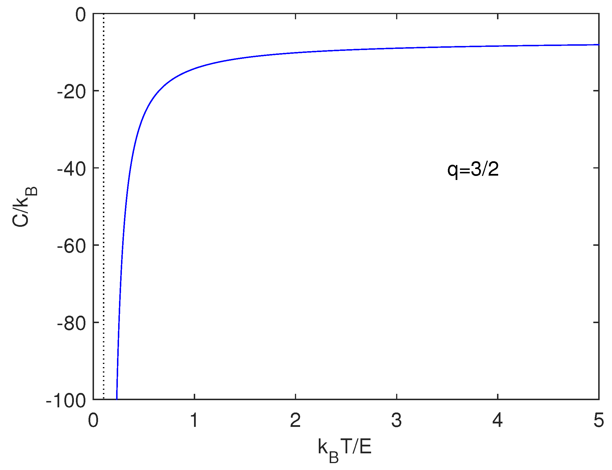
3.2. Predicted Specific Heat

We look now for a specific heat built up as $\mathcal{C}=\frac{\partial \langle \mathcal{U}\rangle }{\partial T}$. For $q=\frac{3}{2}$ we find

$$\begin{gathered} \mathcal{C}=\frac{8k[\ln \left({\pi }^2{G}^2{m}^3{M}^2\right)-4-\ln \left(kT\right)+2\mathit{C}]}{\frac{22}{3}+\ln \left(kT\right)-\ln \left(16{\pi }^2{G}^2{m}^3{M}^2\right)}- \\ \frac{8k[3\ln \left({\pi }^2{G}^2{m}^3{M}^2\right)-3-\ln \left(kT\right)+2\mathit{C}]}{{\left[\frac{22}{3}+\ln \left(kT\right)-\ln \left(16{\pi }^2{G}^2{m}^3{M}^2\right)\right]}^2} \end{gathered}$$

(32)

Figure 1 depicts the specific heat corresponding to Equation (31). One defines $E=G^2{m}^3{M}^2$ with $m\ll M$ and express our quantities in $k_{B}T/E$-units. The specific heat is negative, as Astrophysics indicates for gravitation [1]. This property has been linked to self-gravitational systems [1].

4. Boltzmann-Gibbs Statistics

We pass now to the orthodox statistical formalism, which poses new challenges.

4.1. Analytic Extension

Analytic extension (or continuation) is a technique to extend the domain of a given analytic function. Analytic continuation often succeeds in defining further values of a function, for example in a new region where an infinite series representation in terms of which it is initially defined becomes divergent. Here we should keep in mind that one is dealing with the integral of an exponentially increasing function in $\beta GmM/r$ given by (1).

We appeal in what follows to the use of analytical extension to obtain the result of some useful integrals that we will need later on. The discussion is rather technical and can be skipped without losing sight of our objectives. Whittaker functions play a protagonic role. Such functions are special solutions of Whittaker’s equation, a modified form of the confluent hypergeometric equation. Equations of motion for holonomic systems are Whittaker’s equations (system are called holonomic if all their constraints are holonomic, and a constraint is holonomic if it is expressible as a function).

4.2. Helpful Integrals

Recourse is now to be made to Table [14], where one finds a helpful integral for us, after specializing it. We speak of

$$\underset{0}{\overset{\infty }{\int }}{x}^{\nu -1}{(x+\gamma )}^{\mu -1}{e}^{-\frac{\beta }{x}}dx={\beta }^{\frac{\nu -1}{2}}{\gamma }^{\frac{\nu -1}{2}+\mu }\Gamma (1-\mu -\nu )e^{\frac{\beta }{2\gamma }}{W}_{\frac{\nu -1}{2}+\mu ,-\frac{\nu }{2}}\left(\frac{\beta }{\gamma }\right),$$

(33)

where $\left|\arg \right(\gamma \left)\right|<\pi$. Also, $\Re (1-\mu -\nu )>0$. W is one of the two Whittaker functions. Here we do not demand $\Re \beta >0$, as emphasized by Gradshteyn and Rizhik [14] [see the picture in page 340, Equation (7), named ET II 234(13)a, with reference made to Reference [15] (Caltech’s Bateman Project)]. The final letter “a” stands for analytical extension. Choosing $\mu =1$ one has

$$\underset{0}{\overset{\infty }{\int }}{x}^{\nu -1}{e}^{-\frac{\beta }{x}}dx={\beta }^{\frac{\nu -1}{2}}{\gamma }^{\frac{\nu +1}{2}}\Gamma (-\nu )e^{\frac{\beta }{2\gamma }}{W}_{\frac{\nu +1}{2},-\frac{\nu }{2}}\left(\frac{\beta }{\gamma }\right),$$

(34)

for $\nu \ne 0,-1,-2,-3,.\dots .$ In addition [14],

$$W_{\frac{\nu +1}{2},-\frac{\nu }{2}}\left(\frac{\beta }{\gamma }\right)=M_{\frac{\nu +1}{2},\frac{\nu }{2}}\left(\frac{\beta }{\gamma }\right)={\left(\frac{\beta }{\gamma }\right)}^{\frac{\nu +1}{2}}{e}^{-\frac{\beta }{2\gamma }}.$$

(35)

Here. M is Whittaker’s function two. Thus,

$$\underset{0}{\overset{\infty }{\int }}{x}^{\nu -1}{e}^{-\frac{\beta }{x}}dx={\beta }^{\nu }\Gamma (-\nu ),$$

(36)

which one can evaluate for all $\nu =1,2,3,\dots .$ by recourse to the DR approach [6,7,8,10]. If we turn $\beta$ into $-\beta$ in (33) we have to deal with

$$\underset{0}{\overset{\infty }{\int }}{x}^{\nu -1}{(x+\gamma )}^{\mu -1}{e}^{\frac{\beta }{x}}dx={(-\beta )}^{\frac{\nu -1}{2}}{\gamma }^{\frac{\nu -1}{2}+\mu }\Gamma (1-\mu -\nu )e^{-\frac{\beta }{2\gamma }}{W}_{\frac{\nu -1}{2}+\mu ,-\frac{\nu }{2}}\left(-\frac{\beta }{\gamma }\right).$$

(37)

Again, one chooses $\mu =1$ so that

$$\underset{0}{\overset{\infty }{\int }}{x}^{\nu -1}{e}^{\frac{\beta }{x}}dx={(-\beta )}^{\frac{\nu -1}{2}}{\gamma }^{\frac{\nu +1}{2}}\Gamma (-\nu )e^{-\frac{\beta }{2\gamma }}{W}_{\frac{\nu +1}{2},-\frac{\nu }{2}}\left(-\frac{\beta }{\gamma }\right),$$

(38)

that holds for $\nu \ne 0,-1,-2,-3,\dots \dots$

We tackle now

$$W_{\frac{\nu +1}{2},-\frac{\nu }{2}}\left(-\frac{\beta }{\gamma }\right)=M_{\frac{\nu +1}{2},\frac{\nu }{2}}\left(-\frac{\beta }{\gamma }\right)={\left(-\frac{\beta }{\gamma }\right)}^{\frac{\nu +1}{2}}{e}^{\frac{\beta }{2\gamma }},$$

(39)

plus

$$\underset{0}{\overset{\infty }{\int }}{x}^{\nu -1}{e}^{\frac{\beta }{x}}dx={(-\beta )}^{\nu }\Gamma (-\nu ),$$

(40)

equivalent to interchange $\beta$ with $-\beta$ in (36). We arrive at the fact that restricting the analytical extension (AE) of (33) is the same as effecting the AE of the restriction. This reaffirms that Gradshteyn and Rizhik’s AE is valid. Equation (40) exhibits a cut at $\Re \beta >0$. We are entitled to select then ${(-\beta )}^{\nu }=e^{i\pi \nu }{\beta }^{\nu }$, ${(-\beta )}^{\nu }=e^{-i\pi \nu }{\beta }^{\nu }$, or ${(-\beta )}^{\nu }=\cos \left(\pi \nu \right){\beta }^{\nu }$. We choose the latter possibility and find

$$\underset{0}{\overset{\infty }{\int }}{x}^{\nu -1}{e}^{\frac{\beta }{x}}dx=\cos \left(\pi \nu \right){\beta }^{\nu }\Gamma (-\nu ),$$

(41)

a useful result, to be employed in what follows.

Reference [14] allows us to realize that

$$\underset{0}{\overset{\infty }{\int }}{x}^{\nu -1}{e}^{-\beta x^2-\gamma x}dx={\left(2\beta \right)}^{-\frac{\nu }{2}}\Gamma \left(\nu \right)e^{\frac{{\gamma }^2}{8\beta }}{D}_{-\nu }\left(\frac{\gamma }{\sqrt{2\beta }}\right),$$

(42)

with D being the parabolic-cylinder function. Choosing $\gamma =0$ we encounter

$$\underset{0}{\overset{\infty }{\int }}{x}^{\nu -1}{e}^{-\beta x^2}dx={\left(2\beta \right)}^{-\frac{\nu }{2}}\Gamma \left(\nu \right)D_{-\nu }\left(0\right).$$

(43)

Given that

$$D_{-\nu }\left(0\right)=\frac{2^{-\frac{\nu }{2}}\sqrt{\pi }}{\Gamma \left(\frac{\nu +1}{2}\right)},$$

(44)

one has

$$\underset{0}{\overset{\infty }{\int }}{x}^{\nu -1}{e}^{-\beta x^2}dx=\frac{2^{-\nu }{\beta }^{-\frac{\nu }{2}}\sqrt{\pi }\Gamma \left(\nu \right)}{\Gamma \left(\frac{\nu +1}{2}\right)},$$

(45)

still another helpful result for our future considerations.

5. The $\mathit{\nu }$-Dimensional BG Distribution

The BG partition function ${\mathcal{Z}}_{\nu }$ is well-known (see any text-book on Statistical Mechanics)

$${\mathcal{Z}}_{\nu }=\underset{\mathcal{M}}{\int }{e}^{-\beta \left(\frac{p^2}{2m}-\frac{GmM}{r}\right)}{d}^{\nu }x{d}^{\nu }p,$$

(46)

with $\beta$ the inverse temperature, m and M the involved masses and G the gravitation constant. M is assumed to be at rest at the origin. In effecting the integration process one appeals to hyper-spherical coordinates for the two integrals, each in $\nu$ dimensions. The corresponding change of variables is

$$\begin{gathered} x_1=r\cos {\theta }_1 \\ {x}_2=r\sin {\theta }_1\cos {\theta }_2 \\ {x}_3=r\sin {\theta }_1\sin {\theta }_2\cos {\theta }_3 \\ . \\ . \\ {x}_{\nu -1}=r\sin {\theta }_1\dots \dots \sin {\theta }_{\nu -2}\cos {\theta }_{\nu -1} \\ {x}_{\nu }=\sin {\theta }_1\dots \dots \sin {\theta }_{\nu -1}\sin {\theta }_{\nu -1}, \end{gathered}$$

(47)

where $0\le {\theta }_j\le \pi$, $1\le j\le \nu -2$, and $0\le {\theta }_{\nu -1}\le 2\pi$. The integration on the angular variables (${\mathsf{\Omega }}_{\nu }=({\theta }_1,{\theta }_2,\dots ,{\theta }_{\nu -1})$) yields as a result

$$\underset{{\mathsf{\Omega }}_{\nu }}{\int }d{\mathsf{\Omega }}_{\nu }=\frac{2{\pi }^{\frac{\nu }{2}}}{\Gamma \left(\frac{\nu }{2}\right)}$$

(48)

We are left now with only two radial coordinates (one in r-space, the other in p-space). Then,

$${\mathcal{Z}}_{\nu }={\left[\frac{2{\pi }^{\frac{\nu }{2}}}{\Gamma \left(\frac{\nu }{2}\right)}\right]}^2\underset{0}{\overset{\infty }{\int \int }}{\left(rp\right)}^{\nu -1}{e}^{-\beta \left(\frac{p^2}{2m}-\frac{GmM}{r}\right)}drdp.$$

(49)

At this stage we need (41). Accordingly, $\underset{0}{\overset{\infty }{\int }}{r}^{\nu -1}{e}^{\beta \frac{GmM}{r}}dr$ and (45) for $\underset{0}{\overset{\infty }{\int }}{p}^{\nu -1}{e}^{-\beta \frac{p^2}{2m}}dp,$ so that we obtain

$${\mathcal{Z}}_{\nu }=4\sqrt{\pi }\cos \left(\pi \nu \right){\left(\frac{{\pi }^2\beta G^2{m}^3{M}^2}{2}\right)}^{\frac{\nu }{2}}\frac{\Gamma \left(\nu \right)\Gamma (-\nu )}{{\left[\Gamma \left(\frac{\nu }{2}\right)\right]}^2\Gamma \left(\frac{\nu +1}{2}\right)}.$$

(50)

Looking at (50) one ascertains that poles emerge at any (entire) dimension $\nu$, $\nu =3$ included. Then, appeal to dimensional regularization (DR) to deal with them becomes mandatory. For this we used in Section 4 the generalized DR approach advanced in Reference [10].

Still, we need first an expression for the mean energy

$${\langle \mathcal{U}\rangle }_{\nu }=\frac{1}{{\mathcal{Z}}_{\nu }}\underset{R}{\int }{e}^{-\beta \left(\frac{p^2}{2m}-\frac{GmM}{r}\right)}\left(\frac{p^2}{2m}-\frac{GmM}{r}\right)d^{\nu }x{d}^{\nu }p.$$

(51)

Invoking the hyper-spherical coordinates previously presented we find for ${\langle \mathcal{U}\rangle }_{\nu }$

$${\langle \mathcal{U}\rangle }_{\nu }=\frac{1}{{\mathcal{Z}}_{\nu }}{\left[\frac{2{\pi }^{\frac{\nu }{2}}}{\Gamma \left(\frac{\nu }{2}\right)}\right]}^2\underset{o}{\overset{\infty }{\int \int }}{e}^{-\beta \left(\frac{p^2}{2m}-\frac{GmM}{r}\right)}\left(\frac{p^2}{2m}-\frac{GmM}{r}\right)p^{\nu -1}{r}^{\nu -1}dpdr.$$

(52)

Now, we use again (41) and (45), which gives for the mean energy

$$\begin{gathered} {\langle U\rangle }_{\nu }=\frac{1}{{\mathcal{Z}}_{\nu }}\frac{\sqrt{\pi }}{\beta }\cos \left(\pi \nu \right){\left(\frac{{\pi }^2\beta G^2{m}^3{M}^2}{2}\right)}^{\frac{\nu }{2}}\times \\ \left[\frac{\Gamma (\nu +2)\Gamma (-\nu )}{{\left[\Gamma \left(\frac{\nu }{2}\right)\right]}^2\Gamma \left(\frac{\nu +3}{2}\right)}+4\frac{\Gamma \left(\nu \right)\Gamma (1-\nu )}{{\left[\Gamma \left(\frac{\nu }{2}\right)\right]}^2\Gamma \left(\frac{\nu +1}{2}\right)}\right]. \end{gathered}$$

(53)

In this Section, we have obtained the basic ingredients for working with the canonical ensemble. We now have the partition function for gravity and the mean energy. For them one can obtain the gravitational entropy, first of all, and all the relevant thermodynamic quantities associated with gravity.

5.1. The 3D Regularized BG Distribution

We go back to (50). The idea it to work the ensuing dimensional regularization (DR) process. If we have, for instance, an expression $F\left(\nu \right)$ that diverges, say, for $\nu =3$, our Bollini-Giambiagi’s DR generalized approach consists in performing the Laurent-expansion of F around $\nu =3$ and choose then, as the physical result for F, the $\nu =3$-independent term in that expansion. The justification for this procedure is carefully explained in Reference [10] (see Appendix A).

In our present situation, the pertinent Laurent expansion in $\nu$ (around $\nu =3$) takes the appearance

$$\begin{gathered} {\mathcal{Z}}_{\nu }=-\frac{1}{3\sqrt{\pi }}\left[1+\frac{2}{3(\nu -3)}\right]{\left(2{\pi }^2\beta G^2{m}^3{M}^2\right)}^{\frac{3}{2}}\times \\ \left[\ln \left(2{\pi }^2\beta G^2{m}^3{M}^2\right)+\mathit{C}-\frac{17}{3}\right]+\sum _{s=1}^{\infty }{a}_s{(\nu -3)}^s, \end{gathered}$$

(54)

$\mathit{C}$ standing for Euler’s constant. We see that ${\mathcal{Z}}_{\nu }$ does diverge at $\nu =3$. By fiat (and this is the central tenet of DR), the $(\nu -3)$-independent term in the Laurent expansion of ${\mathcal{Z}}_{\nu }$’s gives the physical value of the $\mathcal{Z}$. Accordingly, from the $\nu$-independent term one finds

$$\mathcal{Z}=\frac{1}{3\sqrt{\pi }}{\left(2{\pi }^2\beta G^2{m}^3{M}^2\right)}^{\frac{3}{2}}\left[\frac{17}{3}-\mathit{C}-\ln \left(8{\pi }^2\beta G^2{m}^3{M}^2\right)\right].$$

(55)

Since $\mathcal{Z}$ is necessarily positive, one encounters a temperature-lower bound

$$T>\frac{e^{-\frac{17}{3}+\mathit{C}}}{k_B}8{\pi }^2{G}^2{m}^3{M}^2,$$

(56)

than can not be perforated.

Analogously, from (53), one obtains for $\langle \mathcal{U}\rangle$ the Laurent expansion

$$\begin{gathered} \mathcal{Z}{\langle \mathcal{U}\rangle }_{\nu }=\frac{8}{\sqrt{\pi }\beta (\nu -3)}{\left(\frac{{\pi }^2\beta G^2{m}^3{M}^2}{2}\right)}^{\frac{3}{2}}+\frac{8}{\sqrt{\pi }\beta }{\left(\frac{{\pi }^2\beta G^2{m}^3{M}^2}{2}\right)}^{\frac{3}{2}}\times \\ \left[\frac{1}{2}\ln \left(\frac{{\pi }^2\beta G^2{m}^3{M}^2}{2}\right)+2\ln 2+\frac{\mathit{C}}{2}-\frac{5}{2}\right]+\sum _{s=1}^{\infty }{a}_s{(\nu -3)}^s, \end{gathered}$$

(57)

where $\mathcal{Z}$ is that of Equation (55). As above, the $(\nu -3)$-independent term is the physical value of the mean energy $\langle \mathcal{U}\rangle$

$$\langle \mathcal{U}\rangle =\frac{1}{\mathcal{Z}}\frac{8}{\sqrt{\pi }\beta }{\left(\frac{{\pi }^2\beta G^2{m}^3{M}^2}{2}\right)}^{\frac{3}{2}}\left[\frac{1}{2}\ln \left(\frac{{\pi }^2\beta G^2{m}^3{M}^2}{2}\right)+2\ln 2+\frac{\mathit{C}}{2}-\frac{5}{2}\right].$$

(58)

Replacing here $\mathcal{Z}$’s physical value provided by Equation (55) we can write

$$\langle \mathcal{U}\rangle =-\frac{3}{2\beta }\frac{\ln \left({\pi }^2\beta G^2{m}^3{M}^2\right)+3\ln 2+\mathit{C}-5}{\ln \left({\pi }^2\beta G^2{m}^3{M}^2\right)+\ln 8+\mathit{C}-\frac{17}{3}}.$$

(59)

We have thus obtained finite gravitational values for the partition function and the mean energy. From them, we get of course all remaining thermodynamic quantities.

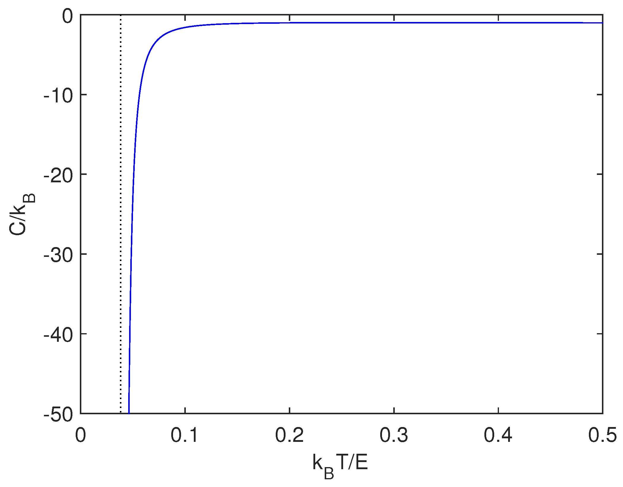
5.2. BG Specific Heat

In Reference [12], the authors derived a canonical gravitational mean energy function. It is natural to now use it for computing the specific heat $\mathcal{C}=\frac{\partial \langle \mathcal{U}\rangle }{\partial T}$. This entails dealing with

$$\begin{gathered} \mathcal{C}=\frac{3k}{2}\frac{\ln \left({\pi }^2\beta G^2{m}^3{M}^2\right)+3\ln 2-6+\mathit{C}}{\frac{17}{3}-\mathit{C}-\ln \left(2{\pi }^2\beta G^2{m}^3{M}^2\right)-\ln 2}- \\ \frac{3k}{2}\frac{\ln \left(16{\pi }^2\beta G^2{m}^3{M}^2\right)+3\ln 2-5+\mathit{C}}{{\left[\frac{17}{3}-\mathit{C}-\ln \left(2{\pi }^2\beta G^2{m}^3{M}^2\right)-\ln 2\right]}^2}. \end{gathered}$$

(60)

Figure 2 displays $\mathcal{C}$ as given by Equation (60). Let us call $E=G^2{m}^3{M}^2$, with $m\ll M$ and express our quantities in $k_{B}T/E$-units. $\mathcal{C}$ turns out to be negative, as astrophysicists expect for gravitation [1]. Certainly, in astrophysics this fact is associated with self-gravitating systems [1]. Thirring did magnificently illustrate negative heat capacities [16,17]. In another vein, Verlinde has linked this sort of system with an entropic force [18]. It should seem natural to then guess that such an entropic force may appear at the energy-associated poles discussed above.

6. Conclusions

It is a common belief that the gravitational partition function $\mathcal{Z}$ linked to a Boltzmann-Gibbs (BG) probability distribution does diverge [1,2].

Here, we tried to undermine this belief as false and circumvented the problem by contemplating the possibility of dimensional regularization. Analytical extension plus dimensional regularization (DR) allows one to encounter finite $\mathcal{Z}$ (see Appendix A).

In preparation for dealing with the Boltzmann-Gibbs approach we worked out the pertinent, easier Tsallis problem and investigated the poles both in its Tsallis’ $\mathcal{Z}$ and in the average energy. These poles emerge at specific, discrete q-values. We studied the thermodynamic behavior at the poles and encountered notable peculiarities. Having succeeded in this Tsallis case, we tackled the orthodox Boltzmann-Gibbs (BG) case and were able to successfully remove the emerging singularities.

The treatment of the gravitational problem is considerably more difficult in the BG than in the Tsallis scenario. The latter only requires dimensional regularization. For BG we need analytic extension as well.

It is important to emphasize that our generalized DR treatment of Reference [10], not the original DR formulation, is the treatment that allows one to bypass divergences in the canonical ensemble Newtonian $\mathcal{Z}$.

References

- Lynden-Bell, D.; Lynden-Bell, R.M. On the negative specific heat paradox. Mon. Not. R. Astron. Soc. 1977, 181, 405–419. [Google Scholar] [CrossRef]
- Padmanabhan, T. Statistical mechanics of gravitating systems. Phys. Rep. 1990, 188, 285–362. [Google Scholar] [CrossRef]
- Padmanabhan, T. Statistical Mechanics of gravitating systems in static and cosmological backgrounds. In Dynamics and Thermodynamics of Systems with Long-Range Interactions; Dauxois, T., Ruffo, S., Arimondo, E., Wilkens, M., Eds.; Springer: Berlin/Heidelberg, Germany, 2002. [Google Scholar]
- Padmanabhan, T. Theoretical Astrophysics: Volume 1, Astrophysical Processes; Cambridge University Press: Cambridge, UK, 2000; Chapter 10. [Google Scholar]
- Binney, J.; Tremaine, S. Galactic Dynamics; Princeton University Press: Princeton, NJ, USA, 1987. [Google Scholar]
- Bollini, C.G.; Giambiagi, J.J. Lowest order “divergent” graps in ν-dimensional space. Phys. Lett. B 1972, 40, 566–568. [Google Scholar] [CrossRef]
- Bollini, C.G.; Giambiagi, J.J. Dimensional Renorinalization: The Number of Dimensions as a Regularizing Parameter. Nuovo Cim. B 1972, 12, 20–26. [Google Scholar]
- Bollini, C.G.; Giambiagi, J.J. Dimensional Regularization in Configuration Space. Phys. Rev. D 1996, 53, 5761. [Google Scholar] [CrossRef]
- Bietenholz, W.; Prado, L. Revolutionary physics in reactionary Argentina. Phys. Today 2014, 67, 38–43. [Google Scholar] [CrossRef]
- Plastino, A.; Rocca, M.C. Quantum Field Theory, Feynman and Wheeler Propagators, Dimensional Regularization in Configuration Space and Convolution of Laurent Invariant Distributions. J. Phys. Commun. 2018, 2, 115029. [Google Scholar] [CrossRef]
- Zamora, J.D.; Rocca, M.C.; Plastino, A.; Ferri, G.L. Application of a dimensionally regularized Tsallis’ Statistical Mechanics to Newton’s gravitation. Physica A 2018, 497, 310–318. [Google Scholar] [CrossRef]
- Rocca, M.C.; Plastino, A.; Ferri, G.L.; Zamora, D. Dimensionally regularized Boltzmann-Gibbs Statistical Mechanics and two-body Newton’s gravitation. Physica A 2018, 503, 793–799. [Google Scholar]
- Tsallis, C. Introduction to Nonextensive Statistical Mechanics Approaching a Complex World; Springer: New York, NY, USA, 2009. [Google Scholar]
- Gradshteyn, I.S.; Rizhik, I.M. Table of Integrals Series and Products; Academic Press: New York, NY, USA, 1965. [Google Scholar]
- Erdelyi, A. Tables of Integral Tranforms; McGraw Hill: New York, NY, USA, 1954; Volume II. [Google Scholar]
- Thirring, W. Systems with negative specific heat. Zeitschrift für Physik A Hadrons and Nuclei 1970, 235, 339–352. [Google Scholar] [CrossRef]
- Thirring, W. The Story of Negative Specific Heat. Paths of Discovery, Pontifical Academy of Sciences, Acta 18, Vatican City. 2006. Available online: http://www.pas.va/content/dam/accademia/pdf/acta18/acta18-thirring.pdf (accessed on 11 July 2019).
- Verlinde, E. On the Origin of Gravity and the Laws of Newton. J. High Energy Phys. 2011, 2011, 29. [Google Scholar] [CrossRef]
- Bollini, C.G.; Escobar, T.; Rocca, M.C. Convolution of Ultradistributions and Field Theory. Int. J. Theor. Phys. 1999, 38, 2315–2332. [Google Scholar] [CrossRef]
- Bollini, C.G.; Rocca, M.C. Convolution of Lorentz Invariant Ultradistributions and Field Theory. Int. J. Theor. Phys. 2004, 43, 1019–1051. [Google Scholar] [CrossRef]
- Bollini, C.G.; Rocca, M.C. Convolution of Even Ultradistribution and Field Theory. Int. J. Theor. Phys. 2004, 43, 59. [Google Scholar] [CrossRef]
- Bollini, C.G.; Marchiano, P.; Rocca, M.C. Convolution of Ultradistributions, Field Theory, Lorentz Invariance and Resonances. Int. J. Theor. Phys. 2007, 46, 3030–3059. [Google Scholar] [CrossRef][Green Version]
- Silva, J.S.E. Les fonctions analytiques comme ultra-distributions dans le calcul opérationnel. Math. Ann. 1958, 136, 58–96. [Google Scholar] [CrossRef]
- Schwartz, L. Théorie des Distributions; Hermann: Paris, France, 1966. [Google Scholar]
- Gel’fand, I.M.; Shilov, G.E. Generalized Functions; Academic Press: New York, NY, USA, 1964; Volume 1. [Google Scholar]
© 2019 by the authors. Licensee MDPI, Basel, Switzerland. This article is an open access article distributed under the terms and conditions of the Creative Commons Attribution (CC BY) license (http://creativecommons.org/licenses/by/4.0/).
be a vertical band contained in the complex -plane
. Integral (A6) is an analytic function of defined in the domain