A Fault Detection Method Based on CPSO-Improved KICA


Abstract
1. Introduction
2. Monitoring Method Using CPSO-KICA
2.1. Principle of CPSO-KICA
2.1.1. KICA
2.1.2. The Selection of Fitness Function
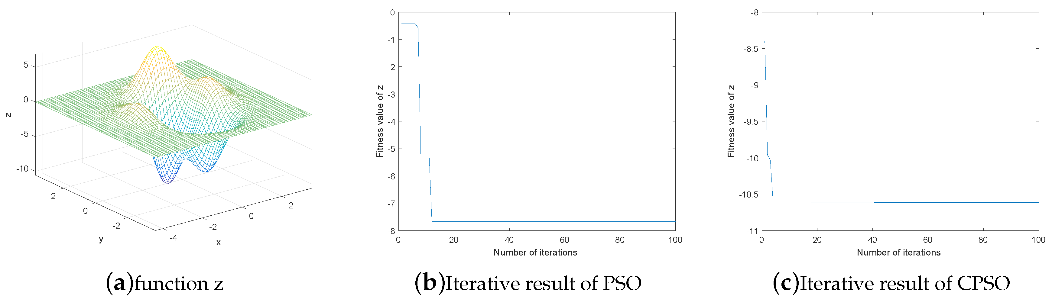
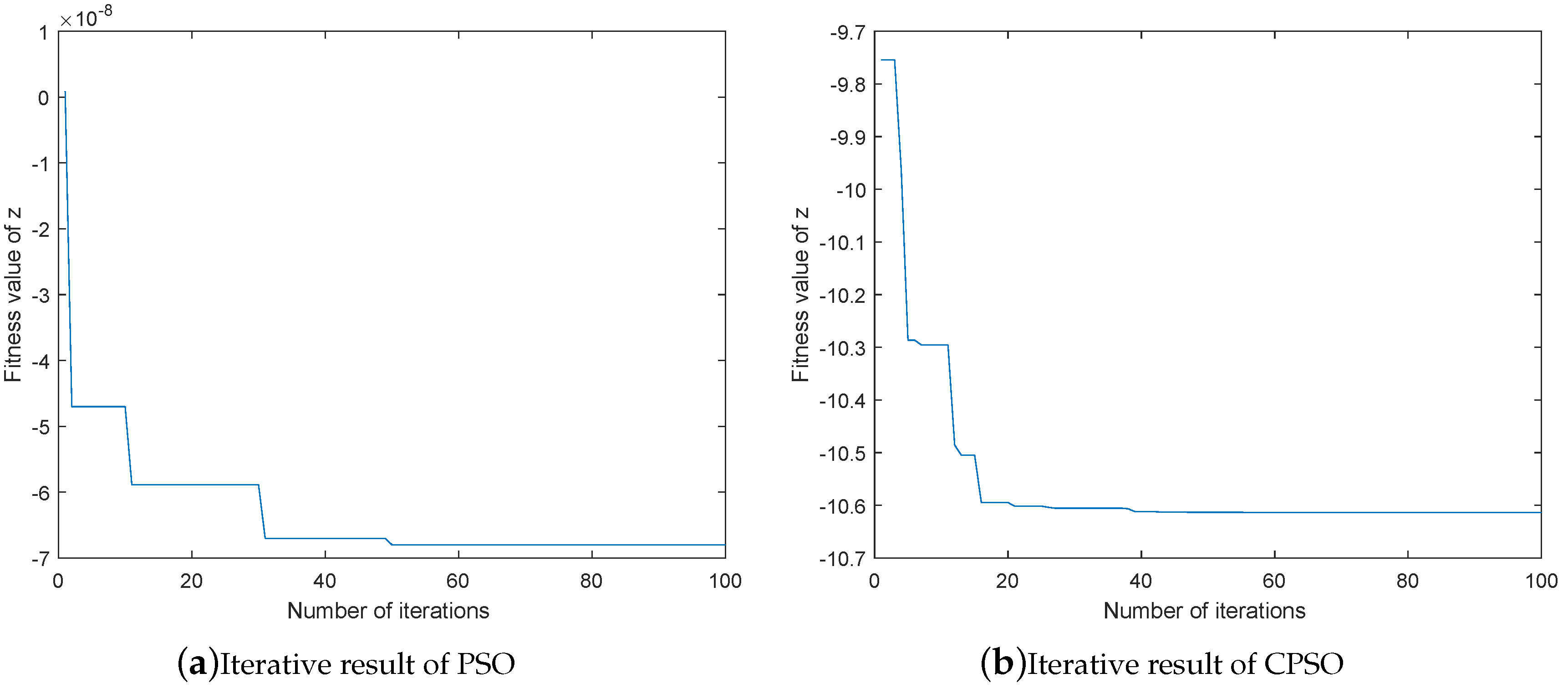
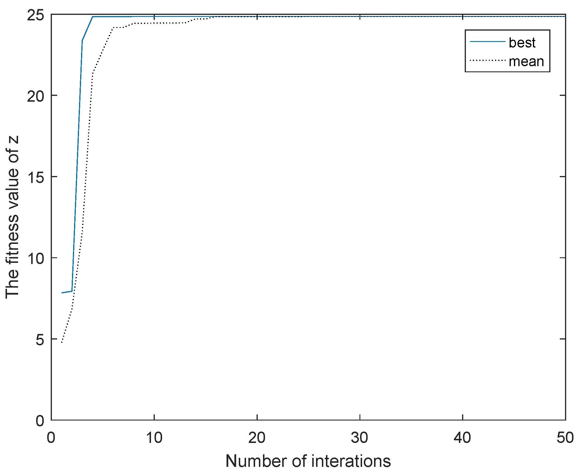
2.1.3. CPSO
2.2. The Process Monitoring Methods
3. Simulation
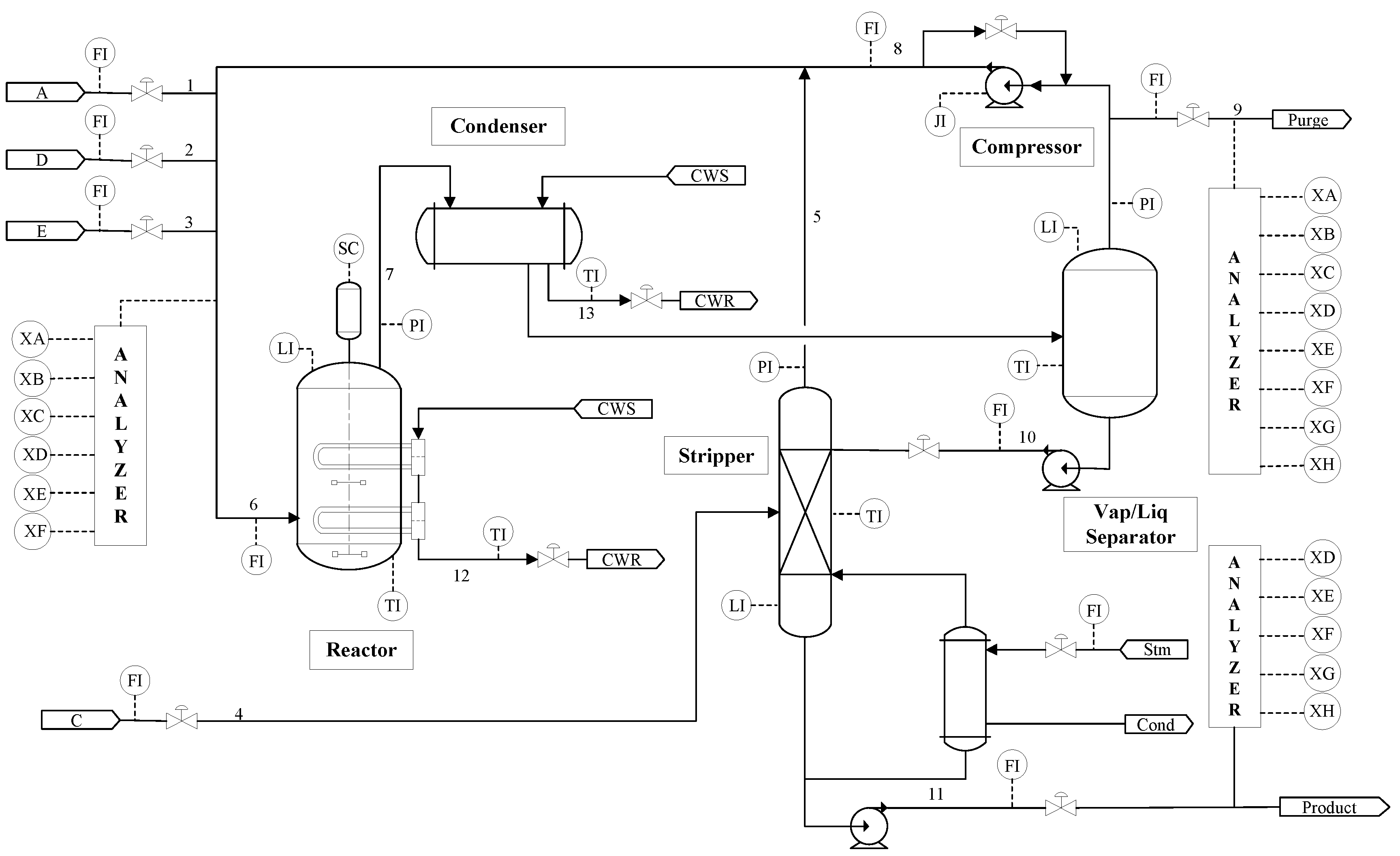
3.1. Data Acquisition
3.2. Results of the Experiment
4. Conclusions
Author Contributions
Funding
Acknowledgments
Conflicts of Interest
References
- Zeng, J.; Xie, L.; Kruger, U.; Gao, C. Regression-Based Analysis of Multivariate Non-Gaussian Datasets for Diagnosing Abnormal Situations in Chemical Processes. AIChE J. 2013, 60, 148–159. [Google Scholar] [CrossRef]
- Santos-Ruiz, J.R.; Bermúdez, F.R.; López-Estrada, V.; Puig, L.; Torres, J.A. Online leak diagnosis in pipelines using an EKF-based and steady-state mixed approach. Control Eng. Pract. 2018, 81, 55–64. [Google Scholar] [CrossRef]
- Santos-Ruiz, J.R.; Bermúdez, F.R.; López-Estrada, V.; Puig, L.; Torres, J.A. Diagnosis of Fluid Leaks in Pipelines Using Dynamic PCA. Int. Fed. Autom. Control. 2018, 51, 373–380. [Google Scholar] [CrossRef]
- Lee, J.M.; Qin, S.J.; Lee, I.B. Fault Detection and Diagnosis of Multivariate Process Based on Modified Independent Component Analysis. AIChE J. 2006, 52, 3501–3514. [Google Scholar] [CrossRef]
- Kano, M.; Tanaka, S.; Hasebe, S.; Hashimoto, I.; Ohno, H. Monitoring independent components for fault detection. AIChE J. 2003, 49, 969–976. [Google Scholar] [CrossRef]
- Sharifi, R.; Langari, R. Nonlinear sensor fault diagnosis using mixture of probabilistic PCA models. Mech. Syst. Signal Process. 2017, 85, 638–650. [Google Scholar] [CrossRef]
- Peng, K.; Zhang, K.; He, X.; Li, G.; Yang, X. New kernel independent and principal components analysis-based process monitoring approach with application to hot strip mill process. IET Control Theory Appl. 2014, 8, 1723–1731. [Google Scholar] [CrossRef]
- Du, W.; Fan, Y.; Zhang, Y.; Zhang, J. Fault diagnosis of non-Gaussian process based on FKICA. J. Frankl. Inst. 2016, 354, 318–326. [Google Scholar] [CrossRef]
- Cai, L.; Tian, X.; Chen, S. Monitoring Nonlinear and Non-Gaussian Processes Using Gaussian Mixture Model-Based Weighted Kernel Independent Component Analysis. IEEE Trans. Neural Netw. Learn. Syst. 2017, 28, 122–135. [Google Scholar] [CrossRef]
- Zhu, B.; Cheng, Z.; Wang, H. A Kernel function optimization and selection algorithm based on cost function maximization. IEEE Int. Conf. Imaging Syst. Tech. 2014, 48, 259–263. [Google Scholar]
- Feng, L.; Di, T.; Zhang, Y. HSIC-based Kernel independent component analysis for fault monitoring. Chemom. Intell. Lab. Syst. 2018, 178, 47–55. [Google Scholar] [CrossRef]
- Popovic, M. Research in entropy wonderland: A review of the entropy concept. Therm. Sci. 2017, 22, 12. [Google Scholar]
- Mamta, G.R.; Dutta, M. PSO Based Blind Deconvolution Technique of Image Restoration Using Cepstrum Domain of Motion Blur. Indian J. Sci. Technol. 2018, 10, 1–8. [Google Scholar] [CrossRef]
- Batra, I.; Ghosh, S. An Improved Tent Map-Adaptive Chaotic Particle Swarm Optimization (ITM-CPSO)-Based Novel Approach Toward Security Constraint Optimal Congestion Management. Iran. J. Sci. Technol. Trans. Electr. Eng. 2018, 42, 261–289. [Google Scholar] [CrossRef]
- Zhu, Y.; Gao, J.; Jia, Y.F. Pattern Recognition of Unknown Partial Discharge Based on Improved SVDD. IET Sci. Meas. Technol. 2018, 12, 907–916. [Google Scholar]
- Uslu, F.S.; Binol, H.; Ilarslan, M.; Bal, A. Improving SVDD classification performance on hyperspectral images via correlation based ensemble technique. Opt. Lasers Eng. 2017, 89, 169–177. [Google Scholar] [CrossRef]
- Li, S.; Wen, J. A model-based fault detection and diagnostic methodology based on PCA method and wavelet transform. Energy Build. 2014, 68, 63–71. [Google Scholar] [CrossRef]
- Yunusa-Kaltungo, A.; Sinha, J.K.; Nembhard, A.D. A novel fault diagnosis technique for enhancing maintenance and reliability of rotating machines. Struct. Health Monit. 2015, 6, 604–621. [Google Scholar] [CrossRef]
- Tian, Y.; Du, W.; Qian, F. Fault Detection and Diagnosis for Non-Gaussian Processes with Periodic Disturbance Based on AMRA-ICA. Ind. Chem. Res. 2013, 52, 12082–12107. [Google Scholar] [CrossRef]
- DOWNS; VOGEL. A plant-wide industrial process control problem. Comput. Chem. Eng 1993, 17, 245–255. [Google Scholar] [CrossRef]
- Chiang, L.H.; Russell, E.L.; Braatz, R.D. Fault Detection and Diagnosis in Industrial Systems. Technometrics 2001, 44, 197–198. [Google Scholar]
- Yi, Z.; Etemadi, A. Line-to-Line Fault Detection for Photovoltaic Arrays Based on Multi-resolution Signal Decomposition and Two-stage Support Vector Machine. IEEE Trans. Ind. Electron. 2017, 64, 8546–8556. [Google Scholar] [CrossRef]
- Shen, Y.; Ding, S.X.; Haghani, A.; Hao, H.; Ping, Z. A comparison study of basic data-driven fault diagnosis and process monitoring methods on the benchmark Tennessee Eastman process. J. Process Control 2012, 22, 1567–1581. [Google Scholar]


| Variables | Description |
|---|---|
| XMV(42) | D feed flow (stream 2) |
| XMV(43) | E feed flow (stream 3) |
| XMV(44) | A feed flow (stream 1) |
| XMV(45) | A and C feed flow (stream 4) |
| XMV(46) | Purge valve (stream 9) |
| XMV(47) | Separator pot liquid flow (stream 10) |
| XMV(48) | Stripper liquid product flow (stream 11) |
| XMV(49) | Reactor cooling water valve |
| XMV(50) | Condenser cooling water flow |
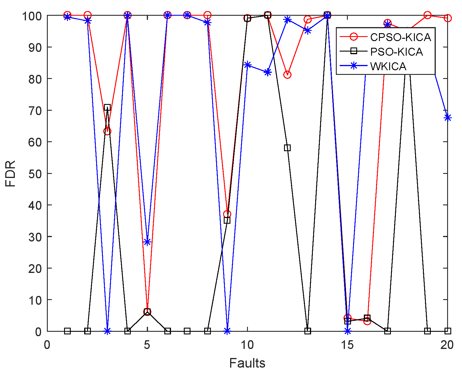
| Fault | WKICA | PSO-KICA | CPSO-KICA | |
|---|---|---|---|---|
| 1 | 99.50 | 99.38 | 0.00 | 100.00 |
| 2 | 98.25 | 98.38 | 0.00 | 100.00 |
| 3 | failed | failed | 71.00 | 63.25 |
| 4 | 99.88 | 91.62 | 0.00 | 100.00 |
| 5 | 28.25 | 25.62 | 6.13 | 6.13 |
| 6 | 100.00 | 100.00 | 0.00 | 100.00 |
| 7 | 100.00 | 99.88 | 0.00 | 100.00 |
| 8 | 97.75 | 97.38 | 0.00 | 100.00 |
| 9 | failed | failed | 35.13 | 37.13 |
| 10 | 84.25 | 79.12 | 99.13 | 99.13 |
| 11 | 82.00 | 50.88 | 100.00 | 100.00 |
| 12 | 98.75 | 99.25 | 58.13 | 82.13 |
| 13 | 95.25 | 94.75 | 0.00 | 98.75 |
| 14 | 99.88 | 99.75 | 100.00 | 100.00 |
| 15 | failed | failed | 3.13 | 4.13 |
| 16 | 90.38 | 78.50 | 4.13 | 3.13 |
| 17 | 97.25 | 91.62 | 0.00 | 97.50 |
| 18 | 90.50 | 89.62 | 93.13 | 94.13 |
| 19 | 89.38 | 54.25 | 0.00 | 100.00 |
| 20 | 67.62 | 54.75 | 0.00 | 99.13 |
| Fault | WKICA | CPSO-KICA | ||
|---|---|---|---|---|
| 1 | 5 | 1.67% | 0 | 0% |
| 2 | 17 | 1.67% | 0 | 0% |
| 3 | failed | 1.67% | 0 | 0% |
| 4 | 2 | 1.67% | 0 | 0% |
| 5 | 1 | 1.67% | 56 | 0% |
| 6 | 0 | 1.67% | 0 | 0% |
| 7 | 0 | 1.67% | 0 | 0% |
| 8 | 19 | 1.67% | 0 | 0% |
| 9 | failed | 1.67% | 16 | 0% |
| 10 | 28 | 1.67% | 7 | 0% |
| 11 | 10 | 1.67% | 0 | 0% |
| 12 | 2 | 1.67% | 7 | 0% |
| 13 | 47 | 1.67% | 5 | 0% |
| 14 | 1 | 1.67% | 0 | 0% |
| 15 | failed | 1.67% | 696 | 0% |
| 16 | 10 | 1.67% | 696 | 0% |
| 17 | 21 | 1.67% | 5 | 0% |
| 18 | 81 | 1.67% | 39 | 0% |
| 19 | 10 | 1.67% | 0 | 0% |
| 20 | 80 | 1.67% | 8 | 0% |
© 2019 by the authors. Licensee MDPI, Basel, Switzerland. This article is an open access article distributed under the terms and conditions of the Creative Commons Attribution (CC BY) license (http://creativecommons.org/licenses/by/4.0/).
Share and Cite
Liu, M.; Li, X.; Lou, C.; Jiang, J. A Fault Detection Method Based on CPSO-Improved KICA. Entropy 2019, 21, 668. https://doi.org/10.3390/e21070668
Liu M, Li X, Lou C, Jiang J. A Fault Detection Method Based on CPSO-Improved KICA. Entropy. 2019; 21(7):668. https://doi.org/10.3390/e21070668
Chicago/Turabian StyleLiu, Mingguang, Xiangshun Li, Chuyue Lou, and Jin Jiang. 2019. "A Fault Detection Method Based on CPSO-Improved KICA" Entropy 21, no. 7: 668. https://doi.org/10.3390/e21070668
APA StyleLiu, M., Li, X., Lou, C., & Jiang, J. (2019). A Fault Detection Method Based on CPSO-Improved KICA. Entropy, 21(7), 668. https://doi.org/10.3390/e21070668