A Thermoelectric-Heat-Pump Employed Active Control Strategy for the Dynamic Cooling Ability Distribution of Liquid Cooling System for the Space Station’s Main Power-Cell-Arrays

Abstract

A proper operating temperature range and an acceptable temperature uniformity are extremely essential for the efficient and safe operation of the Li-ion battery array, which is an important power source of space stations. The single-phase fluid loop is one of the effective approaches for the thermal management of the battery. Due to the limitation that once the structure of the cold plate (CP) is determined, it is difficult to adjust the cooling ability of different locations of the CP dynamically, this may lead to a large temperature difference of the battery array that is attached to the different locations of the CP. This paper presents a micro-channel CP integrated with a thermoelectric heat pump (THP) in order to achieve the dynamic adjustment of the cooling ability of different locations of the CP. The THP functions to balance the heat transfer within the CP, which transports the heat of the high-temperature region to the low-temperature region by regulating the THP current, where a better temperature uniformity of the CP can be achieved. A lumped-parameter model for the proposed system is established to examine the effects of the thermal load and electric current on the dynamic thermal characteristics. In addition, three different thermal control algorithms (basic PID, fuzzy-PID, and BP-PID) are explored to examine the CP’s temperature uniformity performance by adapting the electric current of the THP. The results demonstrate that the temperature difference of the focused CP can be declined by 1.8 K with the assistance of the THP. The proposed fuzzy-PID controller and BP-PID controller present much better performances than that provided by the basic PID controller in terms of overshoot, response time, and steady state error. Such an innovative arrangement will enhance the CP’s dynamic cooling ability distribution effectively, and thus improve the temperature uniformity and operating reliability of the Li-ion space battery array further.

1. Introduction

The Li-ion battery has been proven to be a promising candidate to substitute other energy storage batteries as the power source in space stations [1,2,3] owing to its merits of high power density, high single voltage, long cycling life, environmental friendliness, large operating temperature ranges and so on [4,5,6]. The operation performance of the Li-ion battery array greatly depends on its operating temperature and temperature uniformity. An improper operating temperature may contribute to the reduction in charging efficiency and service life of the batteries [7,8]. Further, an uneven temperature distribution of the single cells may potentially decrease the pack capacity and cause serious safety problems [9]. Accordingly, the battery thermal management system has become an essential approach to enhance the performance of the batteries effectively.

The battery thermal management system has been investigated actively where different cooling technologies, namely air cooling, liquid cooling, heat pipe cooling, and phase change material cooling, were adopted. The air cooling approach [10,11] is classified into natural convection and forced air convection, and the latter is widely researched because of its high convective heat transfer coefficient. The heat pipe cooling [12,13] achieves heat transfer from the heat source to the cooling end to lower the battery array’s temperatur and is largely used in electrical devices for its high effective conductivity. As to the phase change material cooling method, the latent heat of the batteries is stored in the phase change material as the phase changes over a small temperature range, thereby the temperature rise inside the battery can be reduced [14,15]. When confronting more complicated configurations, especially in the case of a large-size high-rate discharging battery array [16], liquid cooling thermal management could manifest better performances than other methods. Furthermore, due to its advantages of strong heat dissipation ability, gravity immunity, structural simplicity, technological maturity, etc., the single-phase fluid loop is regarded as the most promising active approach for Li-ion battery thermal management in space stations.

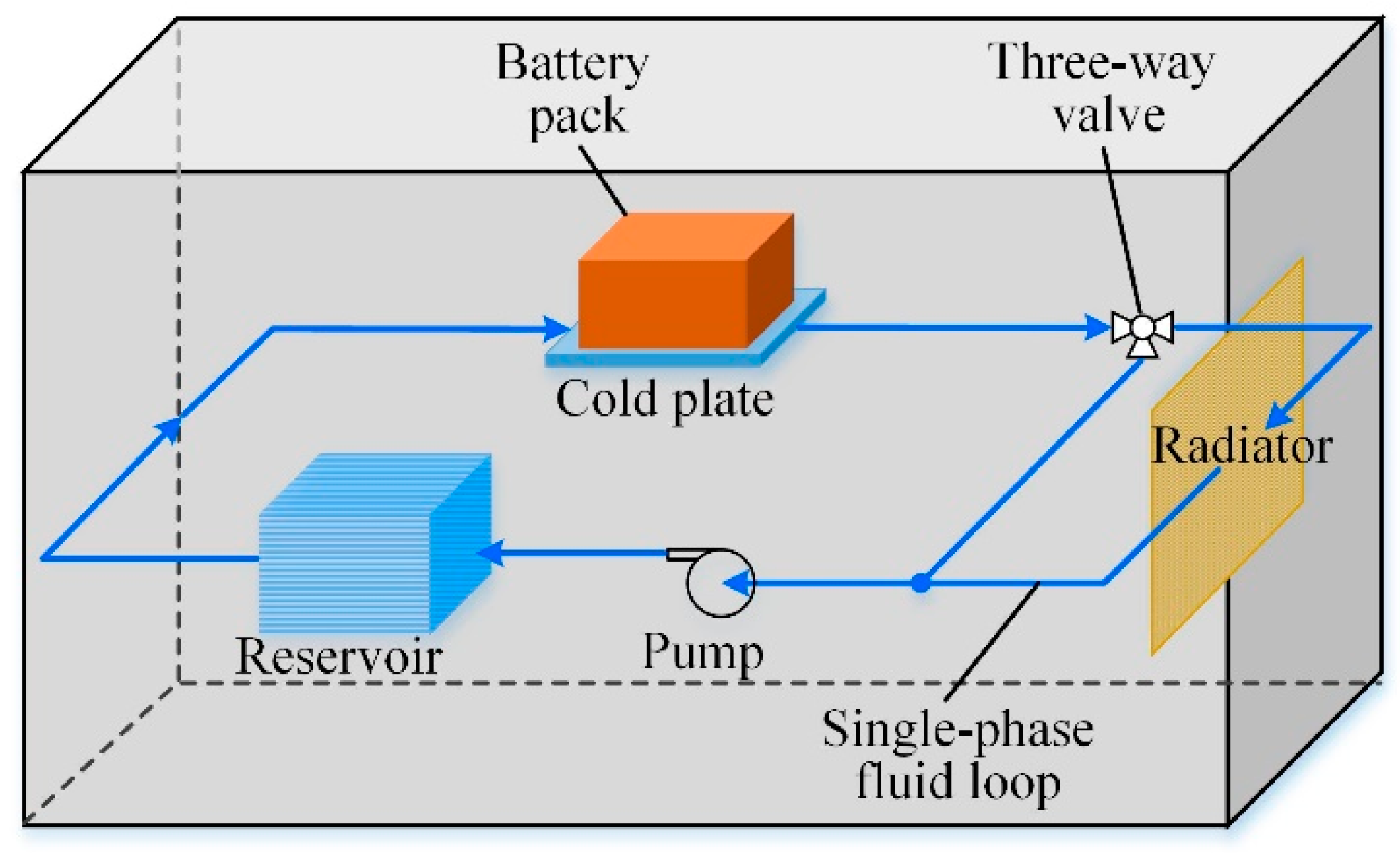
The conventional strategy of the single-phase fluid loop for the space batteries [17] is shown in Figure 1. It comprises of the cold plate (CP), radiator, pump, reservoir and three-way valve. It is shown that the onboard vacuum packaged battery array is cascaded into a single-phase fluid cooling cycle system via a CP. The CP is applied for absorbing the heat generated inside the batteries and the coolant flowing through is for transporting heat to the radiator by which the heat is dissipated to the outer space. To balance the flow through the bypass line and the main fluidic line linking to the radiator, a three-way valve is used by adjusting the valve opening factor between 0% and 100%, through which the coolant temperature can be regulated. The reservoir collects the coolant flowing from the bypass line and the main line for the next cooling cycle, and acts as coolant supplement for the fluid loop when necessary. Undertaking a variety of works, including flow management, heat transfer and energy conversion, etc., the CP is considered to be the key component of the battery liquid cooling system on account of its compactness and ability to separate the battery and fluid [18,19,20].

Much attention has been devoted to the performance improvement of the CP. Yamada et al. [21] developed a honeycomb-cord CP that can obtain a remarkable mass decrease without lowering heat removal capability. Wang et al. [22] designed a silica-plates based cooling system for prismatic lithium-ion batteries during fast charging-discharging process and in specific operating conditions. Jarrett et al. [23] proposed a serpentine-channel CP for the battery liquid cooling system and assessed the effect from the geometry of the channels. The numerical results indicate that with the optimum design, both pressure drop and average temperature can be decreased, but at the expense of temperature uniformity. Wang et al. [24] presented an advanced single phase actively-pumped fluid loop using distributed thermal control strategy applied in spacecraft thermal control system, which included a self-driven CP and a paraffin-actuated thermal control valve. This self-driven control system not only simplified the structure of the conventional mechanically pumped fluid loop effectively, but also improved the operation economy significantly.

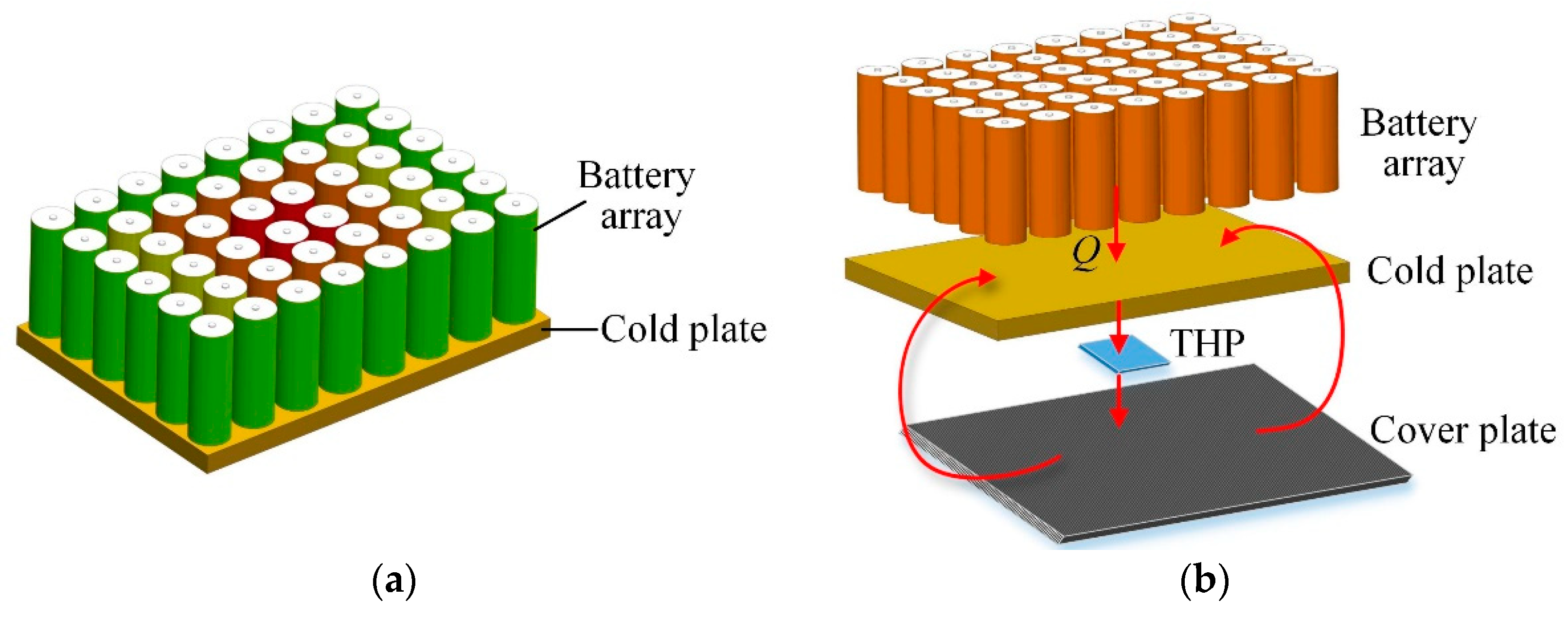
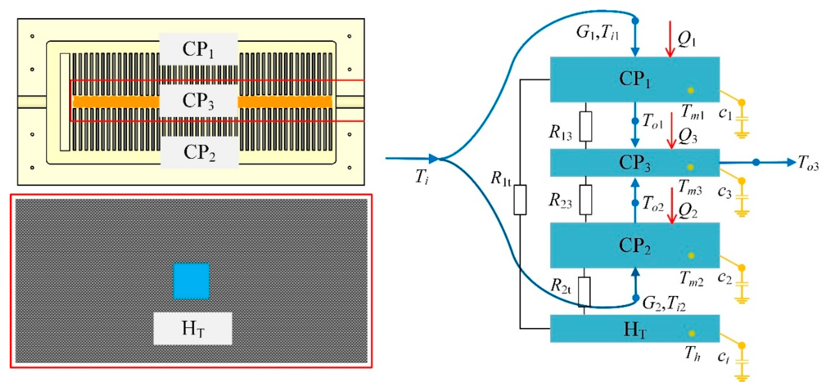
However, few studies focused on the dynamic adjustment of the cooling ability of CP’s different locations which is benefit for the improvement of the overall space battery’s temperature uniformity. As the structure of the CP is fixed, it is difficult to adjust the cooling capacity of the different locations of the CP dynamically which may cause the overheating area or undercooling area. Accordingly, this can directly lead to large temperature difference inside the cells, which is unfavorable for the reliability and capacity utilization of the battery array. As shown in Figure 2a, the temperature of the cells in the middle of the array is much higher than that of the cells on the edge of the CP, which can result in severe temperature unevenness of the power-cell-array and performance degradations or operating failures eventually. Therefore, it is urgent to investigate how to improve the temperature uniformity of the power-cell-array.

To achieve the dynamic cooling ability regulation of different locations of the CP, a thermoelectric heat pump (THP) and a high-heat-conductivity cover plate are employed in this study. Due to the small size, fast cooling speed, no environment pollution, and control simplicity, THPs have been extensively used in the temperature management system [25,26,27]. Traditionally, the cold side of the THP is attached to the cooling object and the hot side of THP the heat sink, which means that the cold-side temperature is usually the only variable can be controlled. The transferred heat in the hot-side heat is dissipated to the external environment space [28,29,30,31]. Nevertheless, different from conventional THP applications, the THP in Figure 2b functions as an effective heat transfer medium through which the heat can be transferred from the high temperature zone to the cover plate firstly. Then the accumulated heat in the cover plate is transferred to the low temperature zone of the CP through heat conduction. Through the function of the THP, the cooling ability of the different locations of the CP can be adjusted dynamically and the temperature uniformity of the power-cell-array can be enhanced notably.

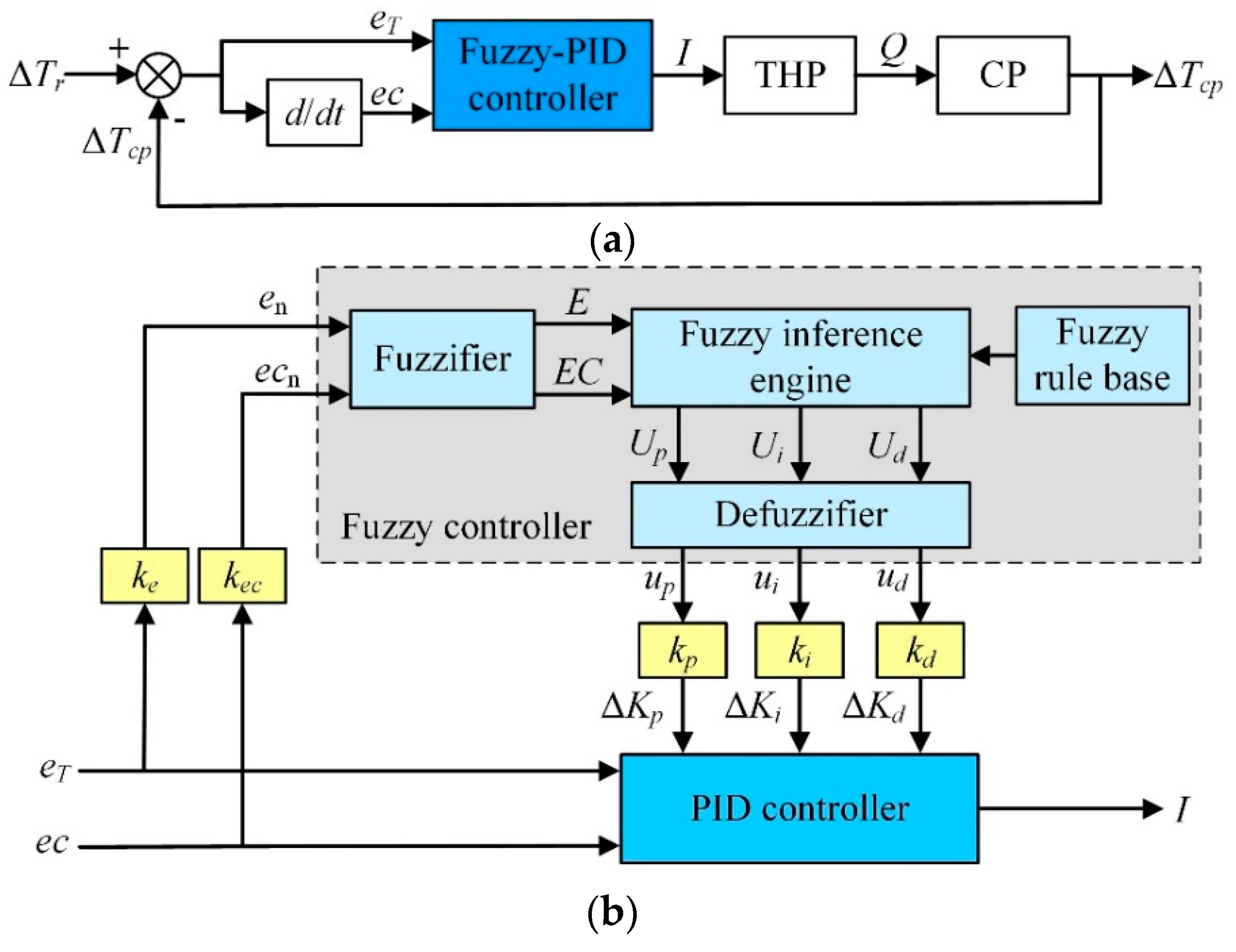
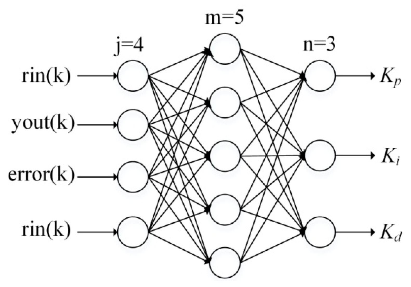
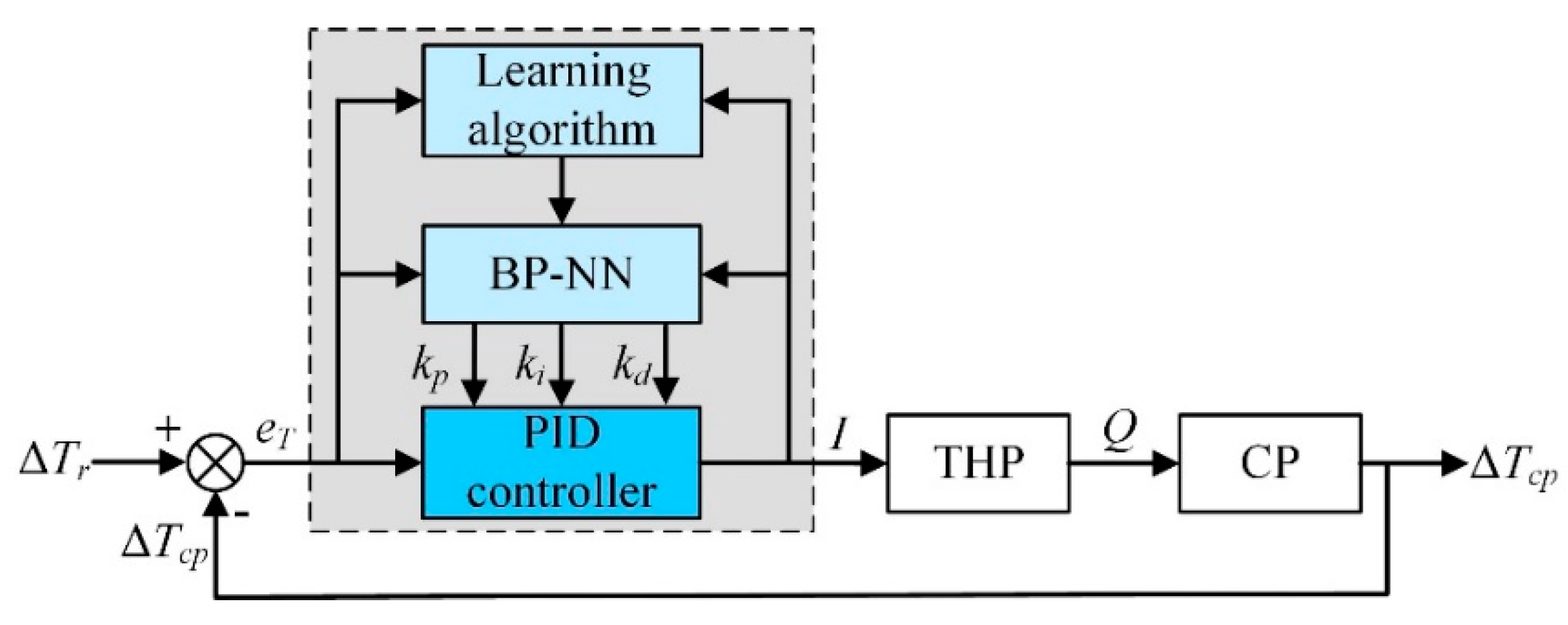
In this paper, an active temperature uniformity control strategy of a novel combined CP-THP system (CCTS) is proposed to improve the temperature uniformity of the CP and finally, the Li-ion space array. A dynamic heat transfer model for the CCTS based on the lumped-parameter method is established. Simulation analyses are conducted to investigate the impacts of the heat load and THP’s electric current on the thermal characteristics of the CP. Three different controllers, namely the basic PID controller, fuzzy-PID controller, and BP-PID controller, are designed to manipulate the CP’s temperature difference by adjusting the electric current passing through the THP. With this THP-based active control strategy, CP’s maximum temperature difference can be decreased, and the temperature uniformity can be improved evidently, which implies that the temperature unevenness of the power-cell-array can be alleviated effectively as well. For further verification, relevant experiments have been conducted and the experimental work will be published in our subsequent paper.

2. System Description and Dynamic Modeling

2.1. General Idea of CCTS

Usually, due to the non-uniformity of the flow pattern in the parallel channels, a clear non-uniform temperature distribution occurs in the CP accordingly which is unfavorable for the temperature uniformity of the space batteries. To alleviate this issue, an adaptive CP module based on the THP is put forward, as described in Figure 3.

The adaptive CP module comprises an aluminum CP, a THP embedded into the lower surface of CP, and a cover plate installed at the bottom of CP. Detailed geometric characteristics of the components of the CP modules are provided in

Table 1. Geometric parameters of CP module.

Parameters (mm)		Value
Cold plate	Outline Size (length × width × height)	600 × 400 × 16
	Wall Thickness	6
	Channel Width	5
	Channel Interval	5
	Channel Height	10
Cover plate	Outline size (length × width × height)	600 × 400 × 2
THP	Outline size (length × width × height)	40 × 40 × 4

. There are two kinds of channel in the CP: (1) multi-fin channels arranged symmetrically and (2) a central channel linking to the outlet. In operation, the working fluid flows from the inlet into the multi-fin channels of both sides. Then these two flows converge into the central channel to be charged out of the CP as a whole through the outlet. Specifically, the cover plate is made of carbon fiber because of its extremely thin thickness, light weight and excellent thermal conductivity, which is of great importance for the system operating in space. Additionally, to guarantee optimal contact among components, the cover plate with eight bolts is capable of sealing the CP perfectly during actual operation.

The configuration of the CCTS is exploded in Figure 4. As described in Figure 2a, the temperature of the batteries in the middle of the array is much higher than that of the batteries on the edge of the array for that the batteries in the middle manifest poor heat dissipation effect, which can also give rise to high temperature in the middle of the CP. Besides, according to the unique channel distribution of CP presented in Figure 3, theoretically there exists the high temperature area corresponding to the central channel in the middle and the low temperature area in the multi-fin channels. The above two reasons both result in temperature non-uniformity of the CP. It will harm the temperature uniformity of the batteries finally. To address this problem, a THP is embedded between the bottom of the CP and the top surface of the cover plate, as also shown in Figure 4, for transferring the heat from the high temperature zone to the low temperature zone of the CP via the carbon fiber plate. Specifically, the cold side of THP is attached to CP’s bottom surface while the hot side to the top surface of the cover plate. In theory, there should be temperature difference between the cold side and the hot side of THP due to the Peltier effect, which means that there may exist temperature difference between the CP and the cover plate. However, owing to the extremely high thermal conductivity and thin thickness of the cover plate, as well as the large contact area between the CP and the cover plate, this temperature difference can be reduced to be negligible.

Considering mainly the effect of heat conduction, we define Q as the thermal load that the battery cells charges into the CP. For temperature acquisition in real time, three temperature sensors are placed on the bottom of CP, which are denoted in Figure 4 as T_m1, T_m2 and T_m3 respectively. To be precise, T_m1 and T_m2 are temperatures of the multi-fin channels on both sides, T_m3 is temperature of the outlet liquid-collecting channel in the middle. Theoretically, T_m1 is identical with T_m2 and both are less than T_m3. Need of special note is that since the cold side of the THP is tightly attached to the middle area of CP’s lower surface, T_m3 is considered to be equal to the cold side temperature of the THP.

The process of counterbalancing the heat is realized by manipulating the electric current that passes through THP. In operation, the electric current input to the THP is adjusted according to the temperature difference among T_m1, T_m2 and T_m3. Therefore, an intelligent controller, as well as a THP driving unit, are designed for simulation.

2.2. Mathematical Modeling

In this section, working mechanism of the CCTS is provided from the point of view of the mathematics and thermodynamics including the lumped-parameter model and the controlling model, which may contribute to a better understanding of the function and dynamic characteristics of the system for the control of its thermal performance.

2.2.1. Lumped-Parameter Model

As shown in Figure 5, a lumped-parameter-based dynamic heat transfer model for the CCTS is proposed to investigate the thermal performance of the CP in detail. In accordance with CP’s channel layout, the multi-fin channels on both sides can be treated as two lumped-parameter nodes which are CP₁ and CP₂ respectively, and the central channel is treated as the third lumped-parameter node CP₃. Besides, the hot side of THP with the cover plate together is considered as the fourth lumped-parameter node H_T similarly, which will be fully described afterwards in this section.

For simplicity, some assumptions are made as follows: (1) the heat transferred from the battery cells to the CP is dominated by heat conduction denoted as thermal load Q; (2) the thermal resistance between the CP and carbon fiber plate is negligible considering the extremely thin thickness and excellent thermal conductivity of the cover plate, as well as large contacting area between the these two components; (3) the thermal resistance between the nodes of CP₁ and CP₂ is also inappreciable because of the small contacting area; (4) the thermal resistance between the node CP₃ and the cold side of THP is considered to be zero for their optimal contact; (5) the initial temperature difference between the hot side and cold side of the THP is 1K.

According to Assumption (2) and Assumption (3), the temperature dynamics of the nodes of CP₁, CP₂, and CP₃, which are based on the energy conservation principle, can be simplified and expressed by Equations (1)–(3).

$$m_1{c}_{cp}\frac{d{T}_{m1}}{d\tau }=Q_1+\frac{1}{R_{13}}\left(T_{m3}-T_{m1}\right)+\frac{1}{R_{1t}}\left(T_h-T_{m1}\right)-c_f{G}_1\eta \left(T_{m1}-T_{i1}\right)$$

(1)

$$m_2{c}_{cp}\frac{d{T}_{m1}}{d\tau }=Q_2+\frac{1}{R_{23}}\left(T_{m3}-T_{m2}\right)+\frac{1}{R_{2t}}\left(T_h-T_{m2}\right)-c_f{G}_2\eta \left(T_{m2}-T_{i2}\right)$$

(2)

$$m_3{c}_{cp}\frac{d{T}_{m3}}{d\tau }=Q_3-\frac{1}{R_{13}}\left(T_{m3}-T_{m1}\right)-\frac{1}{R_{23}}\left(T_{m3}-T_{m2}\right)-c_f{G}_3\eta \left(T_{m3}-T_{i3}\right)-Q_c$$

(3)

where m₁, m₂ and m₃ are the mass of the nodes of CP₁, CP₂ and CP₃ respectively; T_m1, T_m2, T_m3 and T_h are the temperatures of the CP₁, CP₂, CP₃ and the hot side of THP respectively; T_i1, T_i2 and T_i3 are the inlet water temperatures for CP₁, CP₂ and CP₃ respectively; Q is the thermal load of the battery cells; c_cp and c_f are the specific heat of the aluminum-made CP and water as working fluid; R₁₃ and R₂₃ are thermal resistances between CP₁ and CP₃, as well as between CP₂ and CP₃; R_1t and R_2t are thermal resistances between CP₁ and the hot side of THP, as well as between CP₂ and the hot side of THP; G₁, G₂ and G₃ are the mass flow rates of CP₁, CP₂ and CP₃ respectively; η is the heat exchange efficiency. It is noted that due to the symmetry of the two multi-fin channels, all the parameters of CP₁ and CP₂ are considered identical with each other theoretically (namely, m₁ = m₂, T_m1 = T_m2, T_i1 = T_i2, G₁ = G₂, R₁₃ = R₂₃, R_1t = R_2t). Additionally, G₃ is the total mass flow rate coming into the CP which is the sum of G₁ and G₂.

Equations (4) and (5) calculate the output water temperatures from the nodes CP₁ and CP₂ respectively. Equation (6) presents the temperature dynamic equation of the mixing working fluids from the nodes of CP₁ and CP₂. By solving the Equations (1)–(6), we can obtain the temperature of mixing water from nodes of CP₁ and CP₂ (T_fo) which is actually the input water temperature of the node of CP₃ (T_i3) as expressed by Equation (7). Besides, the coolant outlet temperature from the CP is given by Equation (8).

$$T_{o1}=T_{i1}+\eta \left(T_{m1}-T_{i1}\right)$$

(4)

$$T_{o2}=T_{i2}+\eta \left(T_{m2}-T_{i2}\right)$$

(5)

$$\begin{array}{ll}{m}_f{c}_f\frac{d{T}_{fo}}{d\tau }& =\left(G_1{c}_f{T}_{o1}+G_2{c}_f{T}_{o2}\right)-\left(G_1+G_2\right)c_f{T}_{fo}\\ & =G_1{c}_f\left(T_{o1}-T_{fo}\right)+G_2{c}_f\left(T_{o2}-T_{fo}\right)\end{array}$$

(6)

$$T_{i3}=T_{fo}$$

(7)

$$T_{o3}=T_{i3}+\eta \left(T_{m3}-T_{i3}\right)$$

(8)

The temperature dynamics of the node H_T is represented by Equation (9). Therein, the heat flux Q_h charged into the THP hot side can be estimated by Equation (10) and the cooling capacity Q_c in the cold side of the THP which appears in the last term of the Equation (3) is given by Equation (11) where the T_c is the cold-side temperature of the THP which is regarded as equal to that of the node of CP₃ owing to Assumption (4). The power consumption of the THP is expressed by Equation (12). Given the cooling capacity Q_c in Equation (11) and power supply P in Equation (12), the performance of THP can be evaluated by the coefficient of performance (COP) defined in Equation (13). A high COP means less power consumed by the THP, which is of great significance in simulating the CCTS for the operation of Li-ion batteries in the space stations.

$$m_t{c}_t\frac{d{T}_h}{d\tau }=Q_h-\frac{1}{R_{1t}}\left(T_h-T_{m1}\right)-\frac{1}{R_{2t}}\left(T_h-T_{m2}\right)$$

(9)

$$Q_h={\alpha }_t\cdot T_h\cdot I+\frac{1}{2}{I}^2{r}_t-K_t\cdot \left(T_h-T_c\right)$$

(10)

$$Q_c={\alpha }_t\cdot T_c\cdot I-\frac{1}{2}{I}^2{r}_t-K_t\cdot \left(T_h-T_c\right)$$

(11)

where ${\alpha }_t$, R, and K_t are the Seeback coefficient, electrical resistance, and the thermal conductivity of the THP, respectively.

$$P={\alpha }_t\cdot \left(T_h-T_c\right)\cdot I+I^2{r}_t$$

(12)

$$\epsilon =Q_c/P$$

(13)

Given a constant $\mathsf{\Delta }{T}_t$ which is defined in Equation (14), the most suitable current corresponding to the peak value of COP can be attained by Equation (15) with the maximum COP gained by Equation (16) where the M can be acquired by Equation (17).

$$\mathsf{\Delta }{T}_t=T_h-T_c$$

(14)

$$I_{{\epsilon }_{\max }}=\frac{{\alpha }_t\mathsf{\Delta }{T}_t}{\left(M-1\right)r_t}$$

(15)

$${\epsilon }_{\max }=\frac{M{T}_c-T_h}{\mathsf{\Delta }{T}_t\left(M+1\right)}$$

(16)

$$M=\sqrt{1+0.5\left(T_h+T_c\right)}$$

(17)

2.2.2. Control Model

The CCTS is a typical nonlinear system where there are difficulties in reducing the nonlinear constitutive equations to simple linear models while maintaining the accuracy of the respond of the system. To overcome such difficulties, three different control strategies which are basic PID control, fuzzy-PID control, and BP-PID control are proposed in this paper. The PID control serves as a base line for the comparative study with the other two intelligent control strategies. The temperature difference of CP (ΔT_cp), obtained by Equation (18), is selected as the target variable based on which the control variable electric current passing through the THP is adjusted directly and the ΔT_cp is further manipulated by changing heat flux Q_h and cooling capacity Q_c of the THP.

$$\mathsf{\Delta }{T}_{cp}=T_{m3}-T_{m1}=T_{m3}-T_{m2}$$

(18)

Basic PID Controller

The block diagram of the CCTS with the basic PID controller is shown in Figure 6. As the input of the basic PID controller, the control error e_T is the difference between the local temperature difference ΔT_cp and the desired temperature difference ΔT_r described in Equation (19). In this paper, the incremental PID control method is adopted for the basic PID controller, which can be expressed by Equation (20).

$$e_T=\mathsf{\Delta }{T}_{cp}-\mathsf{\Delta }{T}_r$$

(19)

$$\{\begin{array}{l}\mathsf{\Delta }u(t)=K_p\mathsf{\Delta }e(t)+K_{i}e(t)+K_d\left[\mathsf{\Delta }e(t)-\mathsf{\Delta }e(t-1)\right]\\ \mathsf{\Delta }e(t)=e(t)-e(t-1)\end{array}$$

(20)

where u(t) is the incremental output of the controller at the sampling time t; K_p, K_i, K_d are proportional coefficient, integral coefficient and differential coefficient, respectively; e(t) and e(t−1) are the deviation values at the sampling times t and t−1 respectively.

Fuzzy-PID Controller

Figure 7a shows the outline structure of the fuzzy-PID control system. On the basis of conventional PID controller, fuzzy-PID controller adopts the error e_T and error change rate ec as inputs, and the parameters of K_p, K_i, K_d as outputs. Figure 7b shows the detailed structure of the fuzzy-PID controller consisting of a fuzzifier, an inference engine, a defuzzifier, a fuzzy rule-base, and a PID controller. The inputs to the fuzzifier are the error e_n and its changing rate ec_n normalized by the factors k_e and k_ec. Similarly, the outputs of the defuzzifier u_p, u_i, and u_d (scaled by the factors k_p, k_i and k_d) are normalized increments of the controlling parameters K_p, K_i and K_d. The relationships between the parameters (K_p, K_i, K_d) and the inputs (e_T, ec) can be expressed by Equation (21).

$$\{\begin{array}{l}{K}_p=K_{p0}+\{e_T,ec\}{k}_p=K_{p0}+\mathsf{\Delta }{K}_p\\ K_i=K_{i0}+\{e_T,ec\}{k}_i=K_{i0}+\mathsf{\Delta }{K}_i\\ K_d=K_{d0}+\{e_T,ec\}{k}_d=K_{d0}+\mathsf{\Delta }{K}_d\end{array}$$

(21)

where K_p0, K_i0, and K_d0 represent the initial values of K_p, K_i and K_d respectively; ∆K_p, ∆K_i, and ∆K_d are the increments of K_p, K_i and K_d respectively.

The input and output variables of the fuzzy-PID controller are characterized by the fuzzy sets, linguistic values and associated analytical ranks which are listed in

Table 2. Fuzzy sets and their linguistic values.

Fuzzy Sets	Ranks	Linguistic Values
NB	−3	negative high
NM	−2	negative medium
NS	−1	negative low
Z	0	zero
PS	1	positive low
PM	2	positive medium
PB	3	positive high

. Each fuzzy set (or its linguistic value) is defined by various membership functions shown in Figure A1.

The controller output is determined from the linguistic rules in the following form: if en is Ei and ecn is CEj, Then up is Ul(i,j), ui is Um(i,j), ud is Un(i,j). Ei, CEj, Ul(i,j), Um(i,j), and Un(i,j) are the fuzzy values of en, ecn, up, ui, and ud; and the subscript variables i, j, l(i,j), m(i,j) and n(i,j) denote the analytical ranks associated with these linguistic values listed in

Table A1. (a) Fuzzy control rules of ΔK_p. (b) Fuzzy control rules of ΔK_i. (c) Fuzzy control rules of ΔK_d.

(a)
Ei/CEj	NB	NM	NS	Z	PS	PM	PB
NB	PB	PB	PM	PM	PS	Z	Z
NM	PB	PM	PM	PS	PS	Z	NS
NS	PM	PM	PM	PS	Z	NS	NS
Z	PM	PM	PS	Z	NS	NM	NM
PS	PS	PS	Z	NS	NS	NM	NM
PM	PS	Z	NS	NM	NM	NM	NB
PB	Z	Z	NS	NM	NM	NB	NB
(b)
Ei/CEj	NB	NM	NS	Z	PS	PM	PB
NB	NB	NB	NM	NM	NS	Z	Z
NM	NB	NB	NM	NS	NS	Z	Z
NS	NB	NM	NS	NS	Z	PS	PS
Z	NM	NM	NS	Z	PS	PM	PM
PS	NM	NS	Z	PS	PS	PM	PM
PM	Z	Z	PS	PS	PS	PB	PB
PB	Z	Z	PS	PM	PM	PB	PB
(c)
Ei/CEj	NB	NM	NS	Z	PS	PM	PB
NB	PS	NS	NB	NB	NB	NM	PS
NM	PS	NS	NB	NM	NM	NS	Z
NS	Z	NS	NM	NM	NS	NS	Z
Z	Z	NS	NS	NS	NS	NS	Z
PS	Z	Z	Z	Z	Z	Z	Z
PM	PB	NS	PS	PS	PS	PS	PB
PB	PB	PM	PM	PM	PS	PS	PB

. For a two-input system (en and ecn, each with seven fuzzy values), a fully populated rule base will have 7 × 7 = 49 input rule combinations derived with the aid of simulations.

BP-PID Controller

As Figure 8 illustrates, the back propagation PID (BP-PID) controller consists of two parts, the conventional PID controller and the back propagation neural network (BP-NN). The former controller carries on a direct closed-loop control of the THP with the online adjusted K_p, K_i, and K_d obtained by the latter one.

A three-layer BP-NN with four input neuron nodes, five hidden nodes and three output nodes is set up, as shown in Figure 9. As inputs of the input layer, rin(k), yout(k), and error(k) adjust parameters of PID controller K_p, K_i and K_d representing outputs of the output layer according to BP arithmetic.

Due to the input layer is equivalent model, the outputs are equal to the inputs, namely

$$\{\begin{array}{ll}{O}_1^{\left(1\right)}\left(k\right)=rin\left(k\right)& O_2^{\left(1\right)}\left(k\right)=yout\left(k\right)\\ O_3^{\left(1\right)}\left(k\right)=error\left(k\right)& O_4^{\left(1\right)}\left(k\right)=rin\left(k\right)\end{array}$$

(22)

where k is the number of iterations, the superscript (1) refers to the input layer.

The inputs, activation function and outputs of the hidden layer can be expressed by Equations (23)–(25), where the superscript (2) represents the hidden layer, ${\omega }_{jm}^{\left(2\right)}$ is the connection weight from the input layer to the hidden layer defined in Equation (26), $\alpha$ is the learning rate, ${\delta }_m^{\left(2\right)}$ is the local gradient of the hidden layer that is given by Equation (27).

$$ne{t}_m^{\left(2\right)}\left(k\right)={\displaystyle \sum _{j=1}^4{\omega }_{jm}^{\left(2\right)}}{O}_j^{\left(1\right)}\left(k\right),m=1,2,3,4,5$$

(23)

$$f(x)=\left(e^x-e^{-x}\right)/\left(e^x+e^{-x}\right)$$

(24)

$$O_m^{\left(2\right)}\left(k\right)=f\left[ne{t}_m^{\left(2\right)}\left(k\right)\right]$$

(25)

$$\mathsf{\Delta }{\omega }_{jm}^{\left(2\right)}=\alpha {\delta }_m^{\left(2\right)}{O}_j^{\left(1\right)}\left(k\right)$$

(26)

$${\delta }_m^{\left(2\right)}=f^{\prime }\left(ne{t}_m^{\left(2\right)}\left(k\right)\right){\displaystyle \sum _{n=1}^3{\delta }_n^{\left(3\right)}{\omega }_{mn}}$$

(27)

Similarly, the inputs, activation function and outputs of the output layer can be respectively written by Equations (28)–(30), where the superscript (3) represents the output layer, ${\omega }_{mn}^{\left(3\right)}$ is the connection weight from the hidden layer to the output layer which is deduced by Equation (31), ${\delta }_n^{\left(3\right)}$ is the local gradient of the output layer that can be expressed by Equation (32), and $d_n\left(k\right)$ is the desired output of the network. As previously mentioned, the output nodes of the output layer correspond to three adjustable parameters k_p, k_i, and k_d, that is $O_1^{\left(3\right)}=k_p$, $O_2^{\left(3\right)}=k_i$, $O_3^{\left(3\right)}=k_d$. Since these parameters cannot be negative, the activation function of the output layer takes non-negative sigmoid function as Equation (29) describes.

$$ne{t}_n^{\left(3\right)}\left(k\right)={\displaystyle \sum _{m=1}^5{\omega }_{mn}^{\left(3\right)}}{O}_m^{\left(2\right)}\left(k\right),n=1,2,3$$

(28)

$$g(x)=1/\left(1+e^{-x}\right)$$

(29)

$$O_n^{\left(3\right)}\left(k\right)=g\left[ne{t}_n^{\left(3\right)}\left(k\right)\right]$$

(30)

$$\mathsf{\Delta }{\omega }_{mn}^{\left(3\right)}=\alpha {\delta }_n^{\left(3\right)}{O}_m^{\left(2\right)}\left(k\right)$$

(31)

$${\delta }_n^{\left(3\right)}=e_n\left(k\right)g^{\prime }\left(ne{t}_n^{\left(3\right)}\left(k\right)\right)=\left(d_n\left(k\right)-O_n^{\left(3\right)}\right)g^{\prime }\left(ne{t}_n^{\left(3\right)}\left(k\right)\right)$$

(32)

The learning rate is 0.7, and the inertia coefficient is 0.03 for simulation. The initial values of the connection weight coefficients distribute randomly on the interval from −1 to 1, as described in detail in

Table A2. Weight coefficients distribution of BP-NN.

Weight Coefficients	Values
${\omega }_{jm}^{\left(2\right)}$	0.1870		0.3630		−0.3492		−0.1723
	−0.1957		0.4927		−0.3608		−0.1611
	0.5682		−0.0258		0.0277		0.7030
	−0.2202		0.0786		0.2271		0.2690
	0.0357		−0.0086		−0.1074		−0.2447
${\omega }_{mn}^{\left(3\right)}$	0.5776	0.2809		−0.3780		−0.3311		−0.3680
	0.2400	0.2654		−0.1383		0.4525		0.3335
	−0.1706	−0.2657		−0.2839		−0.2201		0.1361

.

2.2.3. Solution Procedure and Simulation Condition Arrangement

As shown in Figure 10, the CP is divided into three domains artificially corresponding to the three lumped-parameter nodes of the focused CP established in Section 2.2.1 (CP₁, CP₂, and CP₃). To be more specific, the three parts account for 25%, 50%, and 25% of the total area of the CP. The initial temperatures of CP₁, CP₂, and CP₃ are presented in Figure 10 as well, which are 297.85 K for CP₁, 297.85 K for CP₂, and 300.85 K for CP₃ respectively. Notice that the initial temperature difference of CP (ΔT_cp) is 3 K. The initial temperature of the THP are also preset as follows, in line with the partition setting of the CP. The cold-side temperature T_c is set as 300.85 K which is identical with T_m3 according to Assumption (4), and the hot-side temperature T_h is set as 301.85 K according to Assumption (5).

Related parameter determinations of the CCTS and the initial state of the system are summarized in

Table 3. Parameter determination of the CCTS.

Parameter (Unit)	Symbol	Value
Cold-plate
Thermal load (W)	Qi	630
Mass (kg)	mcp	6.8
Specific heat (J∙kg−1∙K−1)	ccp	924
Heat exchange efficiency	η	0.9
Heat resistance (K/W)	R13, R23	0.171
	R1t, R2t	0.067
Working fluid
Mass (kg)	mf	0.828
Specific heat (J∙kg−1∙K−1)	cf	4200
Mass flow rate(kg/s)	G	0.02
Inlet temperature (K)	Ti	293
THP
Electric current (A)	I	0
Seeback coefficient (W/K/A)	αt	0.052
Electrical resistance (Ω)	rt	0.9
Thermal conductance (W/K)	Kt	1.182
Heat capacity (J/K).	mtct	619.8

where the thermal load of the batteries (Q_i) and electric current of the THP (I) are critical input parameters as the main inputs for simulation. These two parameters are the primary variables that will be changed and controlled throughout the simulation process. As the base line for transient and control effect analyses, the initial Q_i is 630W, and the initial I is 0 A. Note that in order to take the CP’s heat loss into account, we set the heat exchange efficiency of CP as 0.9.

Matlab R2017a was used as the simulation software. The flowchart of the simulation procedure is shown in Figure 11 which can be described in detail as follows: (1) The program is initialized at the beginning in terms of the physical and working-condition parameters listed in Table 3. (2) The simulation time and the calculation step are preset. (3) The initial temperatures of the CP and THP, T_m1, T_m2, T_m3, T_h and T_c are given. (4) Various input disturbances tabulated in

Table 4. Case arrangement for open-loop dynamic analysis.

Simulation Conditions	Inputs	Final Value	Description	Objective Variable
CP Input Variation	Qi	441W	30% step decrease	Temperature difference of CP
		504 W	20% step decrease
		567 W	10% step decrease
		693 W	10% step increase
		756 W	20% step increase
		819 W	30% step increase
THP Input Variation	I	1A-15A	Increment of 1 A

are applied to the CCTS, beyond which the new value of ΔT_cp can be derived according to Equations (1)–(8) and Equation (22). (5) During the closed-loop control, the control error e_T can be obtained in terms of Equation (23) firstly; and then e_T is transferred into different controllers to calculate the control parameters K_p, K_i and K_d separately by Equations (24)–(36); afterwards the electric current I can be adjusted further; with the adjusted I, Q_h and Q_c brought to the CP will be computed using Equations (9)–(11), leading to a new ΔT_cp finally. (6) After the above procedures, a judgment of whether the simulation time is over will be made. If the simulation time has not reached the set value and the control objective is un-convergence, the relative control algorithm should be modified to adapt the varying input disturbances. The simulation cycle will be updated by the new control parameters.

The focus of this study is to validate that the established CCTS can enhance CP’s temperature uniformity effectively. Two simulation conditions are arranged and listed in Table 4 accordingly. Specifically, a variety of step disturbances in the input Q_i take place in the first simulation condition for demonstrating the influence of the heat load upon the temperature difference of CP. Step disturbances in the THP input current I occur in the second simulation condition to analyze the effect of the THP electric currents on CP’s temperature difference.

Additionally, to investigate the performance in rejecting disturbances of the designed controllers elaborated in Section 2.2.2, three cases (step disturbance, external disturbance and periodic disturbance) in Q_i are organized and listed in

Table 5. Case arrangement for closed-loop control effect analysis.

Simulation Conditions	Inputs	Description	Control Variable	Objective Variable
Step disturbance	Qi	10% step increase at 50s	Electric current of THP	Temperature difference of CP
External disturbance		External disturbance between 600-700W within 900–1000 s
Periodic disturbance		Square wave periodic disturbance with high level of 660 W and low level of 600 W after 200 s

. By evaluating the overshoot, settling time, and steady-state error together, we can evaluate the controlling performance of these three controllers when confronting different system disturbances. Determinations of the control parameters used in the simulation are summarized in

Table A3. Parameters of the simulated controllers.

Controllers	Parameters
Basic PID controller	Kp	Ki	Kd
	12	1	0.5
Fuzzy-PID controller	Kp0	Ki0	Kd0	ke	kec	kp	ki	kd
	12	1	0.5	0.9	0.1	0.3	12	0.1
BP-PID controller	Kp0	Ki0	Kd0	α	β
	12	1	0.5	0.7	0.03

Sample period, T_s = 1.0 s.

.

3. Open-Loop Dynamic Characteristics

The purpose of this section is to investigate the effects of the heat load Q_i and electric current I of THP on the thermal characteristics of the CCTS. Due to the symmetry of multi-fin channels as stated in Section 2.1, T_m2 changes identically with T_m1 under certain condition and both have the same temperature. Therefore, T_m1 is only discussed. The initial value of ΔT_cp (T_m3−T_m2) is 3 K without the operation of the THP. On this basis, all the step-disturbances in Q_i and I take place at 50 s.

3.1. Thermal Load Disturbance

Figure 12 demonstrates the characteristics of the CP under various step disturbances in the thermal load Q_i corresponding to the first simulation condition in Table 4. Note that the heat load is 630 W at the first 50 s, followed by a variety of step-disturbances in an increment of 10% centred on the initial value. In Figure 12a, take the +30% step-disturbance for instance, ΔT_cp rises rapidly from 3 K when the step-disturbance occurs, then it settles to be 3.9 K ultimately which is represented by the blue. For other positive step-disturbance cases, ΔT_cp presents the same trend as well. In contrast, the trend is the opposite for the negative step-disturbance cases. CP’s stable temperature difference (ΔT_{cp_sta}) and the response time τ_r at different Q_i are plotted in Figure 12b. It is obvious that ΔT_{cp_sta} raises linearly at a rate of 4.76 × 10⁻³ K/W with a slight increase in τ_r from 800 s to 1100 s with the increase in Q_i from −30% step-disturbance to +30% step-disturbance. The above observations suggest that more heat load applied to the CP leads to a more severe temperature non-uniformity and a longer settling time. In addition, the temperature difference of the CP is proportional to the heat load.

3.2. Electric Current Disturbance

Figure 13 presents the effect of THP electric current on the temperature changes of the CP. Figure 13a shows three typical step-disturbances of the current (4 A, 8 A and 12 A) upon the ΔT_cp. It is obvious that ΔT_cp in these three cases goes down rapidly to the minimum at about 120 s followed by a slow rise, and then attains a new level of equilibrium finally. The new ΔT_cp is lower than the initial one of 3K.

Figure 13b illustrates the transient temperature curve of T_m1 and T_m3 under the step-disturbance of 12 A. It can be observed that both T_m1 and T_m3 increase in that the power consumption of the THP will be transferred into waste heat which will be applied to the CP finally. To be specific, T_m1 rises sharply and settles to a new steady-state value of 300.65 K under the 12 A step-disturbance at 50 s. Nevertheless, T_m3 declines in a small range at the beginning and escalates to a new stable value of 302.12 K because of Q_c removed from the node of CP₃. Therefore, ΔT_cp reaches a minimum at first and gets to a new stable level finally, which explains that why there exist valley in Figure 13a.

The range of the current step-disturbance is from 1 A to 15 A with the increment of 1 A, ΔT_{cp_sta} varies from 2.79 K to 1.28 K accordingly in Figure 13c where the relationship between ΔT_{cp_sta} and I suggests an approximately negative proportional relationship while the steady-state time τ_r ranges slightly from 700 s to 1200 s and exhibits an increasing trend as a whole. Meanwhile, minimum ΔT_cp in Figure 13d declines from 2.67 K to 0.8 K linearly with the climbing THP current from 1 A to 15 A. Furthermore, the time for minimum ΔT_cp increases quickly at first from 75 s and the increasing rate becomes slow when the time comes to 125 s.

The above observations demonstrate that the THP has a significant effect on the temperature uniformity of the CP absolutely, which is the biggest discovery and innovation in this study. The temperature difference can be reduced by 1.8 K under the maximum current step-disturbance of 15 A of the THP in this paper. However, the higher the current is, the more power the system will consume as expressed in Equation (12). This means more waste heat will be generated which leads to an increase in the overall temperature of the CP. It should be acknowledged that such side-effect is not favorable for the system operation and should be minimized. Therefore, additional discussions in Section 3.3 were carried out to investigate the optimum operating condition of the THP in terms of small temperature difference of the CP and optimum COP of the THP.

3.3. Optimum Operating Conditions of THP

This section aims to determine the optimal range of the control variable I considering the optimal COP with small power consumption which facilitates to depress the excursion of the overall temperature of the CP as shown in Figure 13b, as well as the ΔT_cp which should be small that is crucial for the CCTS.

Before the simulation results being discussed, correlative calculations theoretically should be carried out for further comparison. According to Equations (14) and (15), and the listed parameters of the THP listed in Table 3, the calculated maximal COP ${\epsilon }_{\max }$ is 0.978 and the calculated optimal current for this maximal COP $I_{{\epsilon }_{\max }}$ is 0.996 A on the condition that the ∆T_t remains unchanged of 1K in simulation according to Assumption (5).

Simulation results plotted in the form of ΔT_cp and COP versus I in the range of 0–15 A are presented in Figure 14. It can be seen that ΔT_cp declines gradually with the increasing electric current. The minimum temperature difference is 1.2 K with the maximum current of 15 A. Addtionally, the COP increases rapidly for a small range of the current (0–1 A) and the COP reaches its peak (1.2) when the current is 1 A. After that, the COP decreases gradually to final about 0.4 which is the lowest when the current is 15 A. This simulation result presents a good agreement with the theoretical optimal values ($I_{{\epsilon }_{\max }}=0.996\mathrm{A}$ and ${\epsilon }_{\max }=0.978$).

The observations suggest that higher current (no more than 15 A) results in smaller temperature difference while lower current can obtain a higher COP when the current is within 1–15 A. In this paper, we propose scrupulously that 0.5 is the minimum acceptable COP in the practical operation. Therefore, the THP current is recommended to be controlled below 12 A, and the minimum temperature difference is 1.5 K. On this basis, three strategies are proposed in Section 4 to control the electric current well above a certain COP level (0.5 in this paper) while improving the temperature uniformity of the CP at the same time.

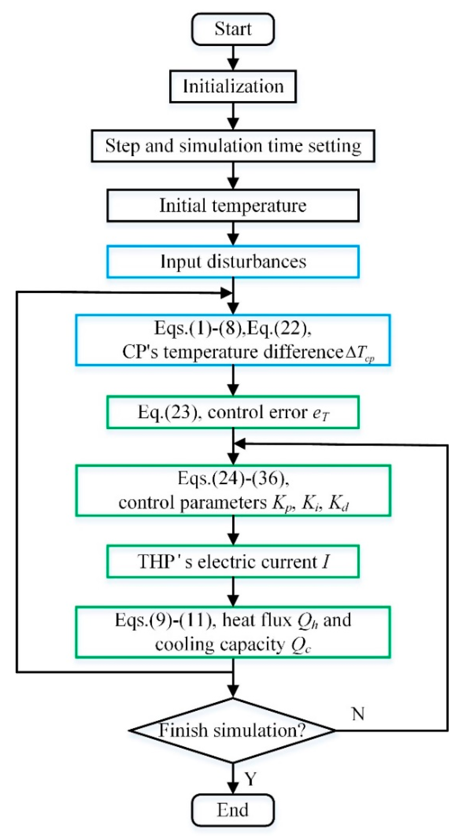
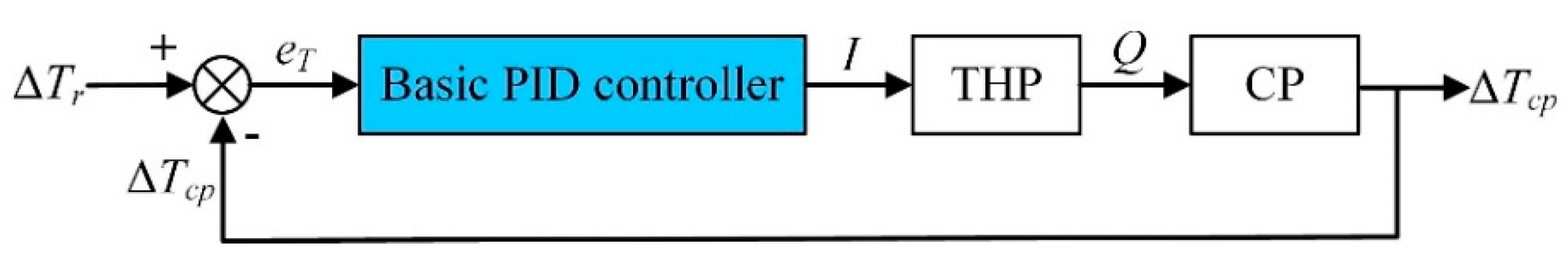
4. Closed-Loop Control Effect Analyses

In this section, the CCTS with three controllers, which are Basic PID, fuzzy-PID, and BP-PID controllers, responses to a variety of disturbances in the thermal load for closed-loop simulation. The results under these three control strategies, which examine the closed-loop control effects, are compared from the parameters such as overshoot, settling time, and steady-state error.

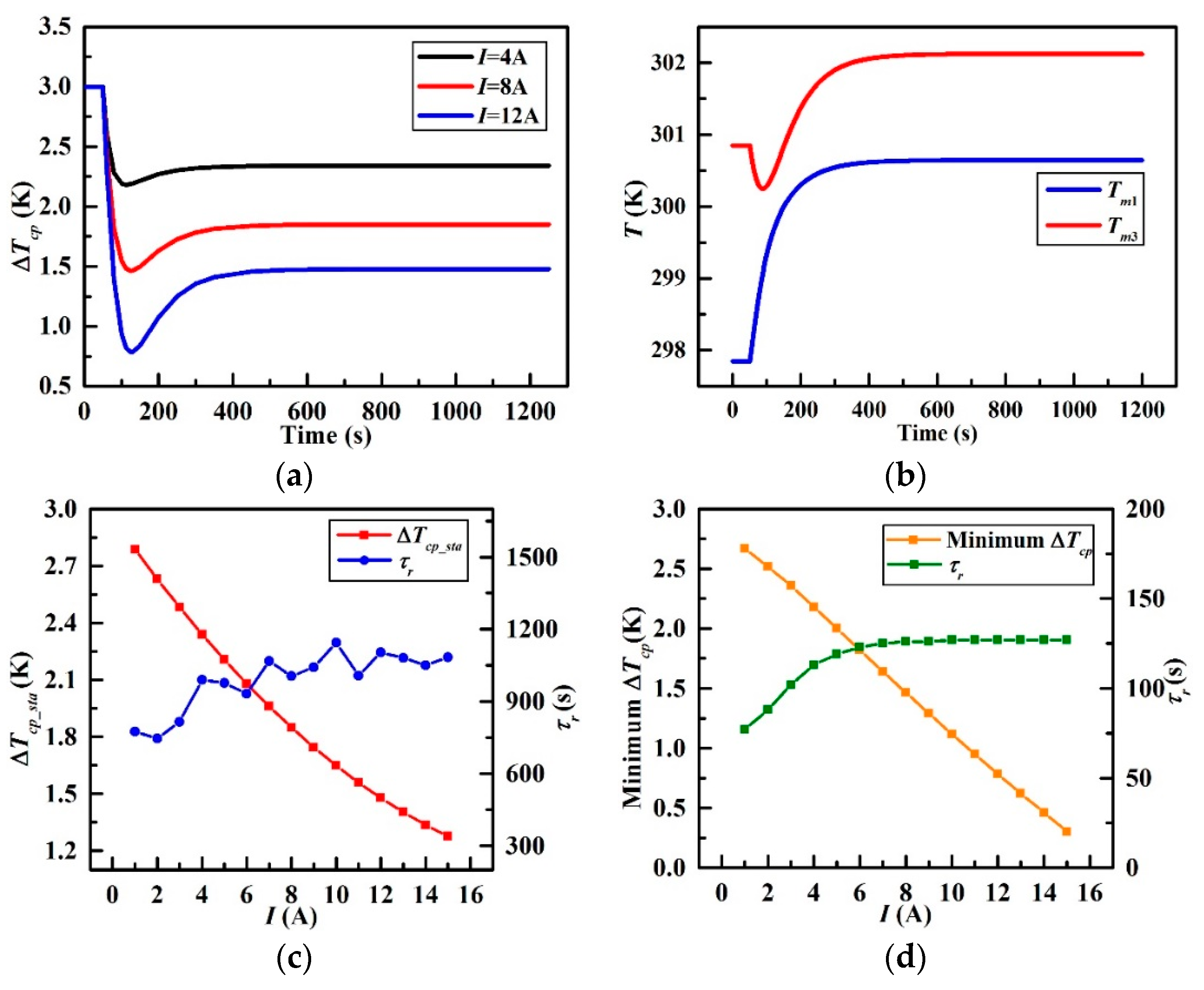
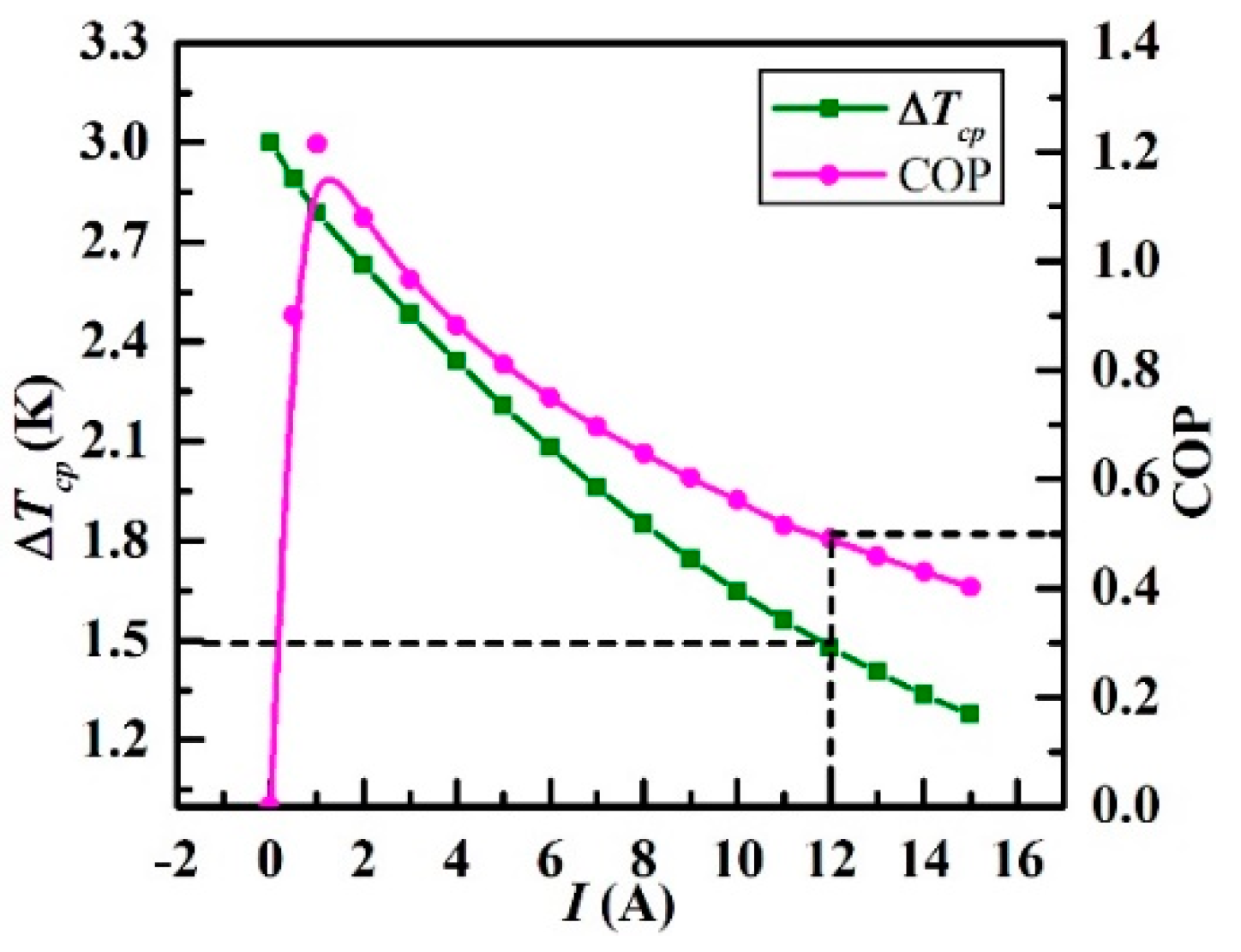
Notice that the desired temperature difference ∆T_r in the closed loop is set to be 1.5 K in this study in that when operated under the current of 12 A as stated in Section 3.3, ΔT_cp was reduced by 1.5 K (from 3 K to 1.5 K). For simplicity, the dynamic temperature difference responses to manipulations from basic PID controller, fuzzy-PID controller, and BP-PID controller are defined as ∆T_{cp_PID}, ∆T_{cp_F} and ∆T_{cp_BP} respectively.

4.1. Step Disturbance Response

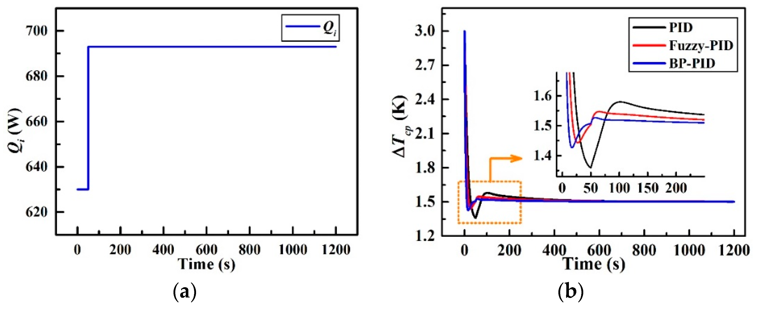
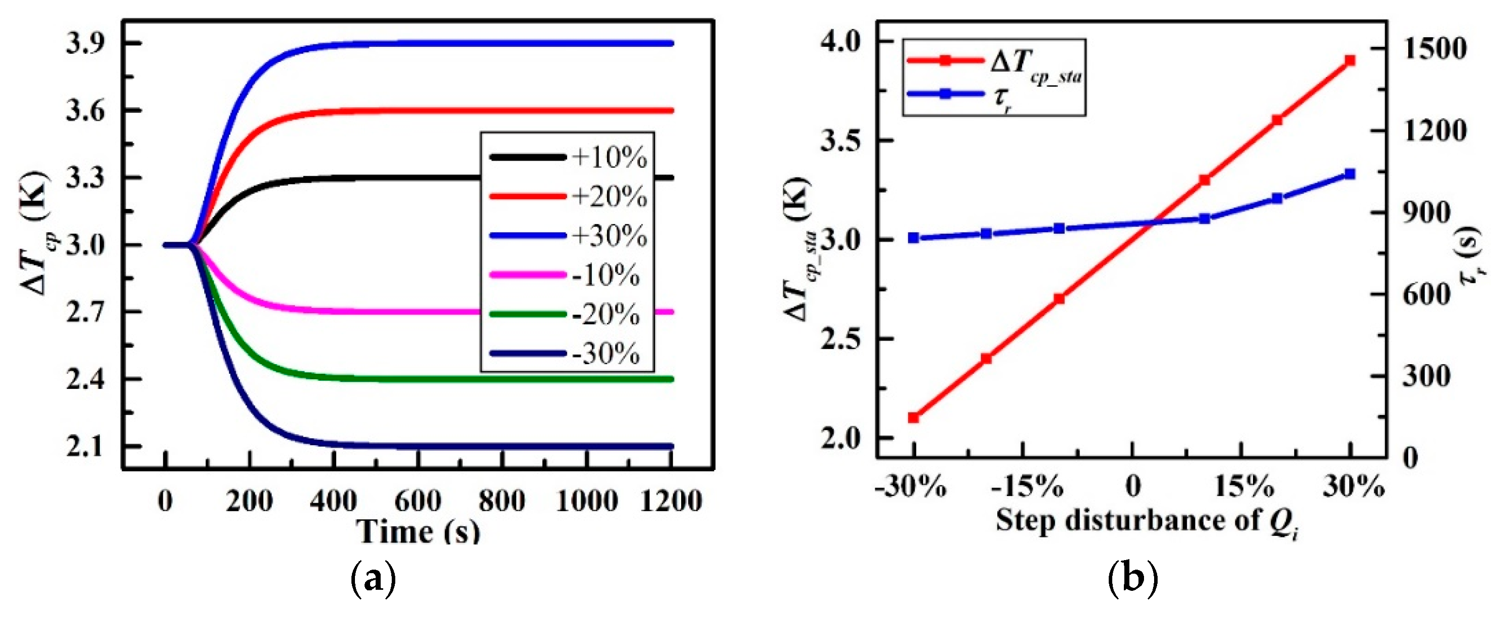
The dynamic temperature difference responses to a 10% step increase in the input heat load Q_i to the CCTS are plotted in Figure 15. As mentioned in Section 3.1, ∆T_cp will climb and settle to a new steady-state value of 3.3 K (0.3 K higher than initial 3 K) without closed-loop control under a +10% step-disturbance in the heat load Q_i at 50 s. As shown in Figure 15b, all the three controllers achieve the objective of 1.5 K. However, there are several specific differences in the control effects among these three control strategies. The closed-loop overshoots γ, settling time τ, and steady-state errors δ of the simulated transients are summarized in

Table 6. Closed-loop control performance parameters for +10% step in Qi.

Controllers	$\mathit{\gamma }(\mathbf{\%})$	$\mathit{\tau }(\mathbf{sec})$	$\mathit{\delta }(\mathbf{\%})$
Basic PID	9.4%	68	0.426%
Fuzzy-PID	3.81%	16	0.073%
BP-PID	4.93%	10	0.033%

. The overshoot, settling time, and steady-state error of the basic PID controller are calculated to be 9.4% (0.14 K), 68 s and 0.426% (0.006 K) respectively as a reference for the comparison. Obviously, the fuzzy-PID controller and BP-PID controller offer a much better temperature dynamic performance than the reference. The overshoot of ∆T_{cp_F} is reduced to 39.1% compared with that of ∆T_{cp_PID}, and the settling time in ∆T_{cp_F} is shortened by 52 s compared with that of ∆T_{cp_PID}. The overshoot of ∆T_{cp_BP} is reduced to 52.4% compared with that of ∆T_{cp_PID}, and the settling time is accelerated by 58 s compared with that of ∆T_{cp_PID}. Besides, the steady-state errors of both ∆T_{cp_F} and ∆T_{cp_BP} are all sufficiently small which can be neglected according to the values in Table 6. Generally, BP-PID controller is better than fuzzy-PID controller from the perspective of the response rate and system stability. In contrast, the latter performs better from the perspective of the maximum overshoot.

4.2. External Disturbance Response

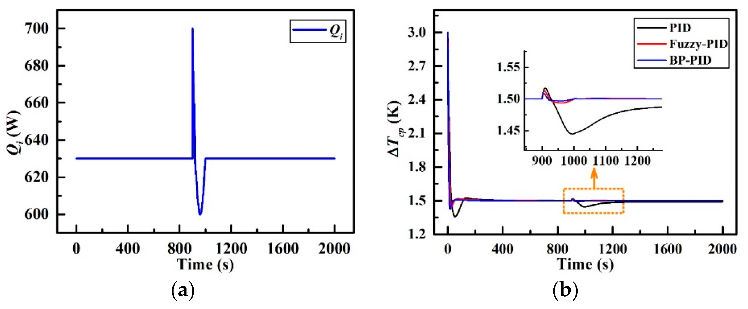
The transient responses of the temperature difference to an unfavorable external disturbance in Q_i are depicted in Figure 16. It can be viewed from Figure 16a that there is a sharp wave pulse disturbance and a half-sinusoid pulse disturbance in the heat load brought from battery cells within 900–1000 s, which may be attributed to the abrupt change in the discharge rate of the Li-ion batteries [32,33,34]. The peak of the sharp wave pulse is 700 W at 900 s and the valley of the half-sinusoid pulse is 600 W at 960 s. As shown in Figure 16b, once the disturbance occurs at 900 s, ∆T_{cp_PID} manifests a fluctuation (maximum overshoot of 0.017 K at 909 s) to the sharp pulse at first and then, a major oscillation (maximum overshoot of 0.055 K at 995 s) to the half-sinusoid pulse, followed by a slow returning at 1000–1300 s. ∆T_{cp_F} and ∆T_{cp_BP}, nevertheless, display just a tiny fluctuation (maximal overshoot of 0.012 K at 907 s and 0.008 K at 905 s respectively) to the sharp pulse with a shorter returning time (20 s and 18 s respectively). In addition, there are no significant responses to the half-sinusoid pulse for these latter two control strategies. The corresponding parameters are listed in

Table 7. Closed-loop control performance parameters for external disturbance in Q_i.

Controllers	$\mathit{\gamma }(\mathbf{\%})$	$\mathit{\tau }(\mathbf{sec})$	$\mathit{\delta }(\mathbf{\%})$
Basic PID	9.48%	86	0.78%
Fuzzy-PID	3.81%	16	0.0067%
BP-PID	4.93%	10	0.0013%

. ∆T_{cp_F} manifests the least maximum overshoot which is 3.81% (0.06 K) while ∆T_{cp_BP} provides the fastest settling time of 10 s compared with that of the other two. With regard to the steady-state performance, the steady-state errors of ∆T_{cp_F} and ∆T_{cp_BP} are both infinitesimally small, and so can be ignored. Therefore, it can be concluded that the fuzzy-PID controller and BP-PID controller present better temperature dynamic ability in responding to unexpected external disturbances as compared to the basic PID controller.

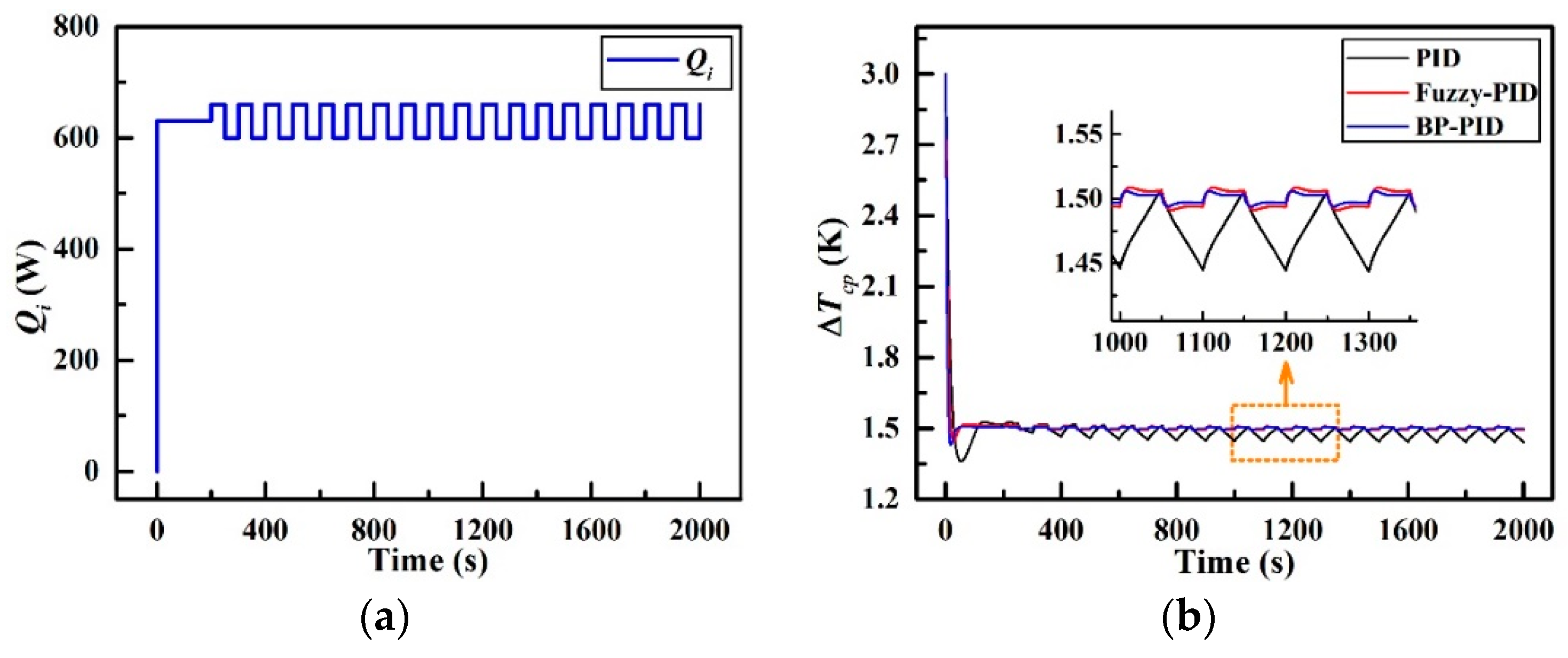
4.3. Periodic Disturbance Response

Figure 17 presents the dynamic temperature difference responses to a periodic disturbance in Q_i. As revealed in Figure 17a, the periodic disturbance in Q_i is simulated in the form of a central constant value of 630 W at the first 200 s and a square wave pulse with high level of 660 W and low level of 600 W respectively after 200 s. The results can be found from Figure 17b that ∆T_{cp_PID} fluctuates within 4% of its steady-state value (the absolute overshoot is 0.06 K) with the settling time of 84 s, while ∆T_{cp_F} fluctuates within 0.53% of its steady-state value (the absolute overshoot is 0.008 K) with the settling time of 16 s. Further, ∆T_{cp_BP} reaches an equilibrium after 10 s with a merely 0.4% fluctuation of its steady-state value (the absolute overshoot is 0.006 K). Additionally, the maximum overshoots of these three controllers are 9.31% (at 53 s), 3.6% (at 27 s), and 4.7% (at 17 s) respectively, and the settling times are 84 s, 16 s and 10 s respectively. All the parameters above can be referred to

Table 8. Closed-loop control performance parameters for periodic disturbance in Q_i.

Controllers	$\mathit{\gamma }(\mathbf{\%})$	$\mathit{\tau }(\mathbf{sec})$	$\mathit{\delta }(\mathbf{\%})$
Basic PID	9.31%	84	4%
Fuzzy-PID	3.6%	16	0.573%
BP-PID	4.7%	10	0.4%

for comparison. The observations suggest that when experiencing a periodical disturbance in the heat load, both fuzzy-PID controller and BP-PID controller still manifest fast response ability and strong self-adaptability as previously expected.

5. Conclusions

For the purpose of actively adjusting the cooling ability of different locations of the cold plate (CP), which is a key component of the single-phase fluid loop, a combined CP-THP system (CCTS) comprising a micro-channel CP integrated with a thermoelectric heat pump (THP) for thermal management of the Li-ion space battery array is proposed to improve the temperature uniformity of the space batteries. The adoption of the THP, which is intended to balance the internal heat transfer within the CP by regulating the THP electric current, is the largest innovation in this paper. The dynamic model for the evaluation of the CP’s thermal characteristics is theoretically established and three control strategies aiming to achieve effective and robust control of the temperature difference within the CP confronting various disturbances are developed. Numerical analyses for both open-loop and closed-loop simulations under different working conditions have been illustrated. Primary conclusions are summarized as follows.

(1)

The maximum temperature difference of the CP was largely influenced by the heat load. Increasing the heat load from the batteries aggravated CP’s temperature unevenness and lengthened the settling time.

(2)

The THP may dynamically adjust the cooling ability of the different locations of the CP and significantly improve the temperature uniformity of the CP under active control strategies. Compared with the traditional module without the THP, the temperature difference of the CP was decreased by 1.8 K with the maximum electric current (15 A) of the THP. The higher electric current was, the better temperature uniformity of the CP can be obtained. Nevertheless, a high electric current may result in unnecessary waste heat which will increase the overall temperature of the CP. Considering the tradeoffs of the temperature difference and power consumption, the electric current should be controlled below 12 A.

(3)

Confronting various conditions of step disturbance, external disturbance and periodic disturbance, both fuzzy-PID and BP-PID controllers achieve an excellent control ability with sufficient fast response and strong stability, which are attractive alternatives to the basic PID controller. Specifically, the fuzzy-PID controller specializes in decreasing overshoot while the BP-PID controller facilitates a reduction of the response time and steady state error.

In conclusion, this THP-based temperature uniformity controlling system can achieve the cooling ability readjustment of different locations of the focused CP, which is extremely benefit for the temperature uniformity improvement of the space battery array. It is expected that this approach would have promising application prospects for other thermal control systems where extremely strict temperature uniformity demands should be satisfied.

References

1. IEC 61960-1. Secondary lithium cell and batteries for portable applications-Part1: Secondary lithium cell. Available online: https://standards.globalspec.com/std/185920/iec-61960-1 (accessed on 9 June 2019).
2. Broussely, M. Lithium batteries R&D activities in Europe. J. Power Sources 1999, 81, 137–139. [Google Scholar]
3. Miao, Y.; Hynan, P.; von Jouanne, A.; Yokochi, A. Current Li-ion battery technologies in electric vehicles and opportunities for advancements. Energies 2019, 12, 1074. [Google Scholar] [CrossRef]
4. Smart, M.; Bugga, R.; Whitcanack, L.; Chin, K.; Surampudi, S.; Gitzendanner, R.; Puglia, F.; Byers, J. Performance testing of lithion 8-cell, 25Ahr lithium-ion batteries for future aerospace applications. In Proceedings of the 1st International Energy Conversion Engineering Conference, Portsmouth, VA, USA, 17–21 August 2003. [Google Scholar]
5. Cutchen, J.T.; Baldwin, A.R.; Levy, S.C. A preliminary evaluation of lithium batteries for extended-life continuous-operation applications. J. Power Sources 1985, 14, 167–172. [Google Scholar] [CrossRef]
6. Soylu, E.; Soylu, T.; Bayir, R. Design and implementation of SOC prediction for a Li-ion battery pack in an electric car with an embedded system. Entropy 2017, 19, 146. [Google Scholar] [CrossRef]
7. Sato, N. Thermal behavior analysis of lithium-ion batteries for electric and hybrid vehicles. J. Power Sources 2001, 99, 70–77. [Google Scholar] [CrossRef]
8. Saw, L.H.; Ye, Y.; Tay, A.A.O. Electrochemical-Thermal Analysis of 18650 Lithium Iron Phosphate Cell. Energy Convers. Manag. 2013, 75, 62–174. [Google Scholar] [CrossRef]
9. Chiu, K.C.; Lin, C.H.; Yeh, S.F.; Lin, Y.H.; Huang, C.S.; Chen, K.C. Cycle life analysis of series connected lithium-ion batteries with temperature difference. J. Power Sources 2014, 263, 75–84. [Google Scholar] [CrossRef]
10. Fan, L.; Khodadadi, J.M.; Pesaran, A.A. Parametric Study on Thermal Management of an Air-Cooled Lithium-Ion Battery Module for Plug-in Hybrid Electric Vehicles. J. Power Sources 2013, 238, 301–312. [Google Scholar] [CrossRef]
11. Wang, T.; Tseng, K.J.; Zhao, J.; Wei, Z. Thermal investigation of lithium-ion battery module with different cell arrangement structures and forced air-cooling strategies. Appl. Energy 2014, 134, 229–238. [Google Scholar] [CrossRef]
12. Zhao, R.; Gu, J.; Liu, J. An experimental study of heat pipe thermal management system with wet cooling method for lithium ion batteries. J. Power Sources 2015, 273, 1089–1097. [Google Scholar] [CrossRef]
13. Tran, T.H.; Harmand, S.; Desmet, B.; Filangi, S. Experimental investigation on the feasibility of heat pipe cooling for HEV/EV lithium-ion battery. Appl. Therm. Eng. 2014, 63, 551–558. [Google Scholar] [CrossRef]
14. Javani, N.; Dincer, I.; Naterer, G.F.; Rohrauer, G.L. Modeling of passive thermal management for electric vehicle battery packs with PCM between cells. Appl. Therm. Eng. 2014, 73, 307–316. [Google Scholar] [CrossRef]
15. Wang, J.X.; Li, Y.Z.; Wang, S.N.; Zhang, H.S.; Ning, X.; Guo, W. Experimental investigation of the thermal control effects of phase change material based packaging strategy for on-board permanent magnet synchronous motors. Energy Convers. Manag. 2016, 123, 232–242. [Google Scholar] [CrossRef]
16. Al-Hallaj, S.; Selman, J.R. Thermal modeling of secondary lithium batteries for electric vehicle/hybrid electric vehicle applications. J. Power Sources 2002, 110, 341–348. [Google Scholar] [CrossRef]
17. Wang, J.X.; Li, Y.Z.; Zhang, H.S.; Wang, S.N.; Liang, Y.H.; Guo, W.; Liu, Y.; Tian, S.P. A highly self-adaptive cold plate for the single-phase mechanically pumped fluid loop for spacecraft thermal management. Energy Convers. Manag. 2016, 111, 57–66. [Google Scholar] [CrossRef]
18. Zhao, L.; Man, G.L.; Cao, J.F. Modeling and simulation on single-phase fluid loop control algorithm. Spacecraft Eng. 2016, 20, 38–43. [Google Scholar]
19. Jin, L.W.; Lee, P.S.; Kong, X.X.; Fan, Y.; Chou, S.K. Ultra-thin minichannel LCP for EV battery thermal management. Appl. Energy 2014, 113, 1786–1794. [Google Scholar] [CrossRef]
20. Bandhauer, T.M.; Garimella, S. Passive, internal thermal management system for batteries using microscale liquid–vapor phase change. Appl. Therm. Eng. 2013, 61, 756–769. [Google Scholar] [CrossRef]
21. Jarrett, A.; Kim, I.Y. Influence of operating conditions on the optimum design of electric vehicle battery cooling plates. J. Power Sources 2014, 245, 644–655. [Google Scholar] [CrossRef]
22. Yamada, H.; Yasuda, T.; Nagasaka, Y.; Okamoto, A.; Ohnishi, A. System studies of advanced single-phase fluid loop with honeycomb-cored cold plate. In Proceedings of the 29th International Conference on Environmental Systems, Denver, CO, USA, 12–15 July 1999. [Google Scholar]
23. Wang, C.; Zhang, G.; Meng, L.; Li, X.; Situ, W.; Lv, Y.; Rao, M. Liquid cooling based on thermal silica plate for battery thermal management system. Int. J. Energy Res. 2017, 41, 2468–2479. [Google Scholar] [CrossRef]
24. Jarrett, A.; Kim, I.Y. Design optimization of electric vehicle battery cooling plates for thermal performance. J. Power Sources 2011, 196, 10359–10368. [Google Scholar] [CrossRef]
25. Rowe, D.M. CRC Handbook of Thermoelectrics; CRC Press: New York, NY, USA, 1995. [Google Scholar]
26. Wang, J.X.; Li, Y.Z.; Mao, Y.F.; Li, E.H.; Ning, X.; Ji, X.Y. Comparative study of the heating surface impact on porous-material-involved spray system for electronic cooling—An experimental approach. Appl. Therm. Eng. 2018, 135, 537–548. [Google Scholar] [CrossRef]
27. Teffah, K.; Zhang, Y.T.; Mou, X.L. Modeling and experimentation of new thermoelectric cooler–thermoelectric generator module. Energies 2018, 11, 576. [Google Scholar] [CrossRef]
28. Zhang, C.W.; Xu, K.J.; Li, L.Y.; Yang, M.Z.; Gao, H.B.; Chen, S.R. Study on a battery thermal management system based on a thermoelectric effect. Energies 2018, 11, 279. [Google Scholar] [CrossRef]
29. Zhang, H.Y.; Mui, Y.C.; Tarin, M. Analysis of thermoelectric cooler performance for high power electronic packages. Appl. Therm. Eng. 2010, 30, 561–568. [Google Scholar] [CrossRef]
30. Wang, J.X.; Li, Y.Z.; Zhang, H.S.; Wang, S.N.; Mao, Y.F.; Zhang, Y.N.; Liang, Y.H. Investigation of a spray cooling system with two nozzles for space application. Appl. Therm. Eng. 2015, 89, 115–124. [Google Scholar] [CrossRef]
31. Sarkar, A.; Mahapatra, S.K. Role of surface radiation on the functionality of thermoelectric cooler with heat sink. Appl. Therm. Eng. 2014, 69, 39–45. [Google Scholar] [CrossRef]
32. Smith, K.; Wang, C.Y. Power and thermal characterization of a lithium-ion battery pack for hybrid-electric vehicles. J. Power Sources 2006, 160, 662–673. [Google Scholar] [CrossRef]
33. Chen, K.W.; Unsworth, G.; Li, X.G. Measurements of heat generation in prismatic Li-ion batteries. J. Power Sources 2014, 261, 28–37. [Google Scholar] [CrossRef]
34. Jeon, D.H.; Baek, S.M. Thermal modeling of cylindrical lithium ion battery during discharge cycle. Energy Convers. Manag. 2011, 52, 2973–2981. [Google Scholar] [CrossRef]
Figure 1. Traditional single-phase fluid loop with CP for Li-ion batteries.
Entropy 21 00578 g001
Figure 2. General design scheme. (a) temperature unevenness of space battery array with traditional single-phase fluid cooling; (b) temperature uniformity improvement of space battery array with proposed approach.
Entropy 21 00578 g002
Figure 3. Construction details of the proposed CP module.
Entropy 21 00578 g003
Figure 4. System configuration.
Entropy 21 00578 g004
Figure 5. Lumped-parameter model.
Entropy 21 00578 g005
Figure 6. Block diagram of basic PID control system.
Entropy 21 00578 g006
Figure 7. Block diagram illustrating CCTS with Fuzzy-PID controller; (a) Control block diagram and (b) Fuzzy-PID controller components.
Entropy 21 00578 g007
Figure 8. Control block diagram of BP-PID controller.
Entropy 21 00578 g008
Figure 9. Structure of BP-NN.
Entropy 21 00578 g009
Figure 10. Partition setting of CP.
Entropy 21 00578 g010
Figure 11. Simulation process flowchart.
Entropy 21 00578 g011
Figure 12. Characteristics under various step disturbances of Qi; (a) ΔTcp versus times and (b) Variations of ΔTcp_sta and τr at different Qi.
Entropy 21 00578 g012
Figure 13. Characteristics of different step changes in I; (a) ΔTcp versus times, (b) Temperature variations at the 12 A step-disturbance, (c) ΔTcp_sta and τr versus I, and (d) Minimum ΔTcp and τr versus I.
Entropy 21 00578 g013
Figure 14. Variations of ΔTcp and COP under different currents.
Entropy 21 00578 g014
Figure 15. Simulated responses to a step-disturbance in Qi; (a) +10% step-disturbance in Qi and (b) transient curve of ∆Tcp.
Entropy 21 00578 g015
Figure 16. Effect of external disturbance in Qi; (a) Qi with external disturbance and (b) Responses of ∆Tcp.
Entropy 21 00578 g016
Figure 17. Temperature responses in the periodical heat load disturbance; (a) Qi with periodic disturbance and (b) ∆Tcp variations.
Entropy 21 00578 g017