1. Introduction
For single or multi terminal source encoding systems, the converse coding theorems state that, at any data compression rates below the fundamental theoretical limit of the system, the error probability of decoding can not go to zero when the block length n of the codes tends to infinity.
In this paper, we study the one helper source coding problem posed and investigated by Ahlswede, Körner [
1] and Wyner [
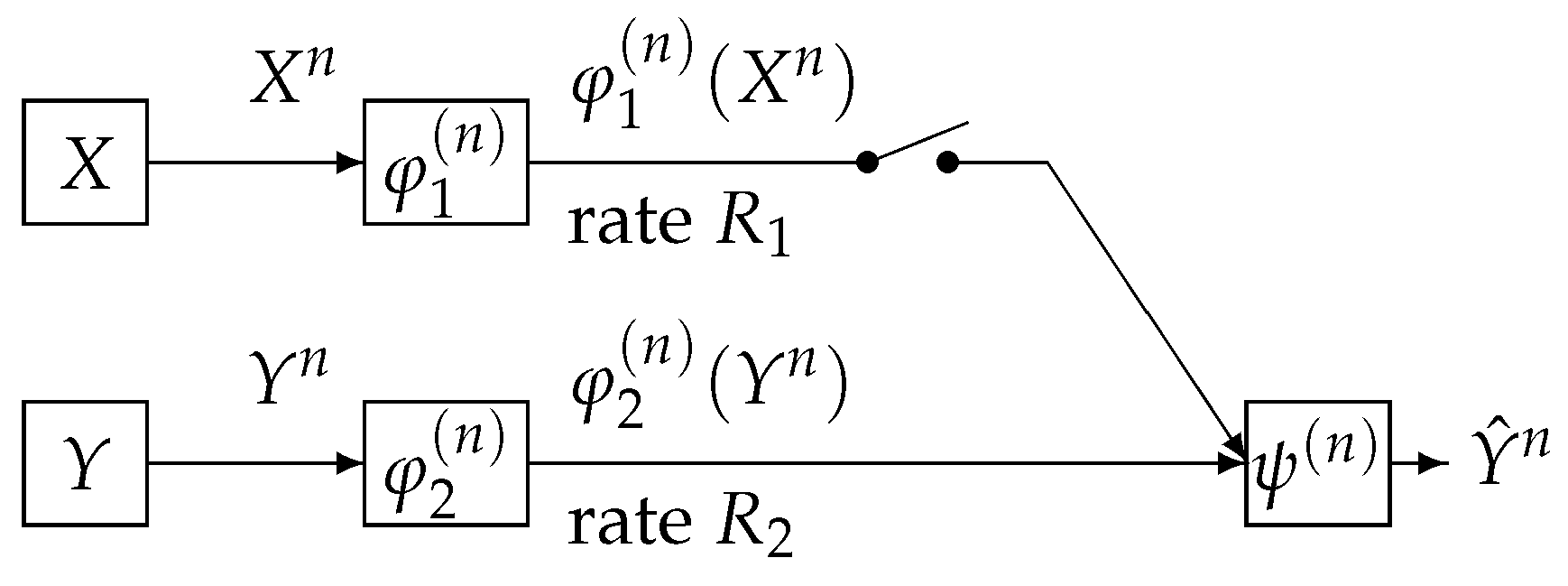
2]. We call the above source coding system (the AKW system). The AKW system is shown in
Figure 1.
In this figure, the AKW system corresponds to the case where the switch is closed. In
Figure 1, the sequence
represents independent copies of a pair of dependent random variables
which take values in the finite sets
, respectively. We assume that
has a probability distribution denoted by
. For each
, the encoder
outputs a binary sequence which appears at a rate
bits per input symbol. The decoder function
observes
and
to output a sequence
, which is an estimation of
. When the switch is open, it is well known that the minimum transmission rate
such that the error probability
of decoding tends to zero as
n tends to infinity is given by
. Csiszár and Longo [
3] proved that, if
, then the correct probability
of decoding decay exponentially and derived the optimal exponent function. When the switch is open and
, Slepian and Wolf [
4] proved that
is the minimum transmission rate
such that the error probability
of decoding tends to zero as
n tends to infinity. Oohama and Han [
5] proved that, if
, then the correct probability
of decoding decay exponentially and derived the optimal exponent function.
In this paper, we consider the strong converse theorem in the case where the switch is closed and
. Let
be the rate region of the AKW system. This region consists of the rate pair
such that the error provability of decoding goes to zero as
n tends to infinity. The rate region was determined by Ahlswede, Körner [
1] and Wyner [
2]. On the converse coding theorem, Ahlswede et al. [
6] proved that, if
is outside the rate region, then,
must tends to zero as
n tends to infinity. Gu and Effors [
7] examined a speed of convergence for
to tend to zero as
by carefully checking the proof of Ahlswede et al. [
6]. However, they could not obtain a result on an explicit form of the exponent function with respect to the code length
n.
Our main results on the strong converse theorem for the AKW system are as follows. For the AKW system, we prove that, if is outside the rate region , must go to zero exponentially and derive an explicit lower bound of this exponent. This result corresponds to Theorem 3. As a corollary from this theorem, we obtain the strong converse result, which is stated in Corollary 2. This result states that we have an outer bound with gap from the rate region .
To derive our result, we use a new method called the recursive method. This method, which is a new method introduced by the author, includes a certain recursive algorithm for a single letterization of exponent functions. In a standard argument of proving converse coding theorems, single letterization methods based on the chain rule of the entropy functions are used. In general, the functions representing multi letter characterizations of exponent functions do not have the chain rule property. In such cases, the recursive method is quite useful for deriving single letterized bounds. The recursive method is a general powerful tool to prove strong converse theorems for several coding problems in information theory. In fact, the recursive method plays important roles in deriving exponential strong converse exponent for communication systems treated in [
8,
9,
10,
11,
12].
On the strong converse theorem for the one helper source coding problem, we have two recent other works [
13,
14]. The above two works proved the strong converse theorem using different methods from our method. In [
13], Watanabe found a relationship between the AKW system and the Gray–Wyner network. Using this relationship and the second order rate region for the Gray–Wyner network obtained by him [
15], Watanabe established the strong converse theorem for the AKW system. In [
14], Liu et al. introduced a new method to derive sharp strong converse bounds via a reverse hypercontractivity. Using this method, they obtained an outer bound of the rate region for the AKW system with
gap from the rate region. Furthermore, in [
14], an extension of the AKW system to the case of Gaussian source and quadratic distortion is investigated, obtaining an outer bound with
gap from the rate distortion region for the extended source coding system. In his resent paper [
16], Liu showed a lower bound (converse) on the dispersion of AWK as the variance of the linear combination of information densities.
The strong converse theorems seem to be regarded just as a mathematical problem and have been investigated mainly from theoretical interest. Recently, Watanabe and Oohama [
17] have found an interesting security problem, which has a close connection with the strong converse theorem for the AKW system. Furthermore, Oohama and Santoso [
18] and Santoso and Oohama [
19] clarify that the exponential strong converse theorem obtained by this paper plays an essential role in deriving a strong sufficient secure condition for the privacy amplification in their new theoritical model of side channel attacks to the Shannon chipher systems. From the above two cases, we expect that exponential strong converse theorems for multiterminal source networks will serve as a strong tool to several information theoretical security problems.
2. Problem Formulation
Let
and
be finite sets and
be a stationary discrete memoryless source. For each
, the random pair
takes values in
, and has a probability distribution
We write
n independent copies of
and
, respectively as
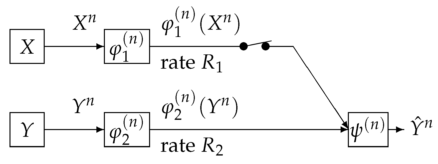
We consider a communication system depicted in
Figure 2. This communication system corresponds to the case where the switch is closed in
Figure 1. Data sequences
and
are separately encoded to
and
and those are sent to the information processing center. At the center, the decoder function
observes
to output the estimation
of
. The encoder functions
and
are defined by
where for each
,
stands for the range of cardinality of
. The decoder function
is defined by
The error probability of decoding is
where
. A rate pair
is
-
achievable if, for any
, there exists a positive integer
and a sequence of triples
such that, for
,
For
, the rate region
is defined by
Furthermore, define
We can show that the two rate regions
,
and
satisfy the following property.
Property 1. - (a)
The regions , , and are closed convex sets of , where - (b)
has another form using -rate region , the definition of which is as follows. We set Using , can be expressed as
Proof of this property is given in
Appendix A. It is well known that
was determined by Ahlswede, Körner and Wyner. To describe their result, we introduce an auxiliary random variable
U taking values in a finite set
. We assume that the joint distribution of
is
The above condition is equivalent to
. Define the set of probability distribution
by
Set
We can show that the region
satisfies the following property.
Property 2. - (a)
The region is a closed convex subset of .
- (b)
The minimum is attained by . This result implies that Furthermore, the point always belongs to .
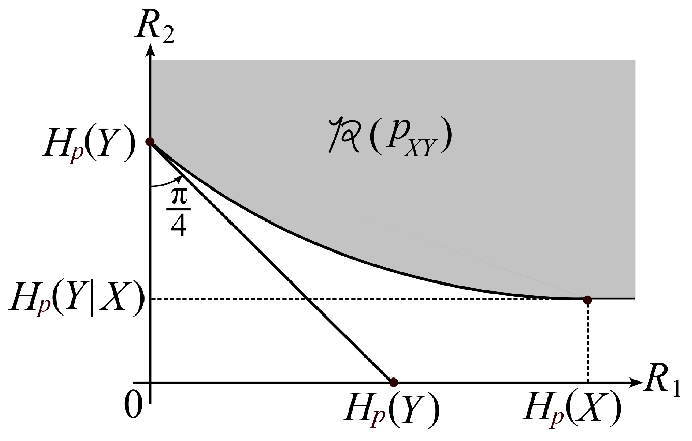
Property 2 part a is a well known property. Proof of Property 2 part b is easy. Proofs of Property 2 parts a and b are omitted. A typical shape of the rate region
is shown in
Figure 3.
The rate region
was determined by Ahlswede and Körner [
1] and Wyner [
2]. Their results are the following.
Theorem 1 (Ahlswede, Körner [
1] and Wyner [
2]).
On the converse coding theorem, Ahlswede et al. [
6] obtained the following.
Theorem 2 (Ahlswede et al. [
6]).
For each fixed ε, we have Gu and Effors [
7] examined a speed of convergence for
to tend to 1 as
by carefully checking the proof of Ahlswede et al. [
6]. However, they could not obtain a result on an explicit form of the exponent function with respect to the code length
n.
Our aim is to find an explicit form of the exponent function for the error probability of decoding to tend to one as
when
. To examine this quantity, we define the following quantity. Set
By time sharing, we have that
Choosing
in the inequality (
5), we obtain the following subadditivity property on
:
from which this, and Fekete’s subadditive lemma, we have that
exists and satisfies the following:
The exponent function
is a convex function of
. In fact, from the inequality (
5), we have that for any
The region
is also a closed convex set. Our main aim is to find an explicit characterization of
. In this paper, we derive an explicit outer bound of
whose section by the plane
coincides with
.
3. Main Results
In this section, we state our main result. We first explain that the region
can be expressed with a family of supporting hyperplanes. To describe this result, we define a set of probability distributions on
by
For
, define
Furthermore, define
Then, we have the following property.
Property 3. - (a)
The bound is sufficient to describe .
- (b)
For every , we have - (c)
Property 3 part a is stated as Lemma A1 in
Appendix B. Proof of this lemma is given in this appendix. Proofs of Property 3 parts b and c are given in
Appendix C. Set
For
, and for
, define
We next define a function serving as a lower bound of
. For
and for
, define
Furthermore, set
We can show that the above functions satisfy the following property.
Property 4. - (a)
The cardinality bound in is sufficient to describe the quantity . Furthermore, the cardinality bound in is sufficient to describe the quantity .
- (b)
For any , we have - (c)
For any and any , we have - (d)
Fix any and . For , we define a probability distribution by Then, for , is twice differentiable. Furthermore, for , we have The second equality implies that is a concave function of .
- (e)
For every , defineand set Then, we have Furthermore, for any , we have - (f)
For every , the condition implieswhere g is the inverse function of .
Property 3 part a is stated as Lemma A2 in
Appendix B. Proof of this lemma is given in this appendix. Proof of Property 4 part b is given in
Appendix D. Proofs of Property 4 parts c, d, e, and f are given in
Appendix E.
Our main result is the following.
Theorem 3. For any , any , and for any satisfying we have It can be seen from Property 4 parts b and f that is strictly positive if is outside the rate region . Hence, by Theorem 3, we have that, if is outside the rate region, then the error probability of decoding goes to one exponentially and its exponent is not below . It immediately follows from Theorem 3 that we have the following corollary.
Proof of Theorem 3 will be given in the next section. The exponent function at rates outside the rate region was derived by Oohama and Han [
5] for the separate source coding problem for correlated sources [
4]. The techniques used by them is a method of types [
21], which is not useful to prove Theorem 3. Some novel techniques based on the information spectrum method introduced by Han [
22] are necessary to prove this theorem.
From Theorem 3 and Property 4 part e, we can obtain an explicit outer bound of
with an asymptotically vanishing deviation from
. The strong converse theorem established by Ahlswede et al. [
6] immediately follows from this corollary. To describe this outer bound, for
, we set
which serves as an outer bound of
. For each fixed
, we define
by
Step (a) follows from
. Since
as
, we have the smallest positive integer
such that
for
. From Theorem 3 and Property 4 part e, we have the following corollary.
Corollary 2. For each fixed ε, we choose the above positive integer . Then, for any , we haveThe above result together withyields that, for each fixed , we haveThis recovers the strong converse theorem proved by Ahlswede et al. [6]. Proof of this corollary will be given in the next section.
4. Proof of the Main Result
Let
be a pair of random variables from the information source. We set
. Joint distribution
of
is given by
It is obvious that
. Then, we have the following lemma, which is well known as a single shot infomation spectrum bound.
Lemma 1. For any and for any , satisfying we haveThe probability distributions appearing in the three inequalities (12), (13), and (14) in the right members of (15) have a property that we can select them as arbitrary. In (12), we can choose any probability distribution on . In (13), we can choose any distribution on . In (14), we can choose any stochastic matrix : . This lemma can be proved by a standard argument in the information spectrum method [
22]. The detail of the proof is given in
Appendix F. Next, we single letterize the four information spectrum quantities inside the first term in the right members of (
15) in Lemma 1 to obtain the following lemma.
Lemma 2. For any and for any , satisfying we havewhere for each , the probability distribution on appearing in (16) and the stochastic matrix appearing in (17) have a property that we can choose their values arbitrary. Proof. In (
12) in Lemma 1, we choose
having the form
In (
13) in Lemma 1, we choose
having the form
We further note that
Then, the bound (
15) in Lemma 1 becomes
completing the proof. □
As in the standard converse coding argument, we identify auxiliary random variables, based on the bound in Lemma 2. The following lemma is necessary for such identification.
Lemma 3. Suppose that, for each , the joint distribution of the random vector is a marginal distribution of . Then, we have the following Markov chain:or equivalently that . Furthermore, we have the following Markov chain:or equivalently that . The above two Markov chains are equivalent to the following one long Markov chain: Proof of this lemma is given in
Appendix G. For
, set
. Define a random variable
by
. From Lemmas 2 and 3, we identify auxiliary random variables to obtain the following lemma.
Lemma 4. For any and for any , satisfying we havewhere, for each , the probability distribution on appearing in (21) and the stochastic matrix appearing in (22) have a property that we can choose their values arbitrary. Now, the challenge is that, although the quantities inside the first term in the right members of (
23) in Lemma 4 have
n sum of information spectrum quantities, the measure
does not have an i.i.d. structure in general. To resolve this, we first use the large deviation theory to upper bound the first quantity in the right members of (
23). For each
, set
Let
be a set of all
. We define a quantity which serves as an exponential upper bound of
. Let
be a set of all probability distributions
on
having a form:
For simplicity of notation, we use the notation
for
. For each
,
is a marginal distribution of
. For
, we simply write
. For
,
,
, and
, we define
where for each
, the probability distribution
and the conditional probability distribution
appearing in the definition of
can be chosen as arbitrary.
The following is well known as the Cramèr’s bound in the large deviation principle.
Lemma 5. For any real valued random variable Z and any , we have By Lemmas 4 and 5, we have the following proposition.
Proposition 1. For any any , and any satisfying there exists such that Proof. By Lemma 4, for
, we have the following chain of inequalities:
Step (a) follows from Lemma 5. When
, the bound we wish to prove is obvious. In the following argument, we assume that
. We choose
so that
Solving (
25) with respect to
, we have
For this choice of
and (
24), we have
completing the proof. □
Set
By Proposition 1, we have the following corollary.
Corollary 3. For any and any satisfying we have We shall call the communication potential. The above corollary implies that the analysis of leads to an establishment of a strong converse theorem for the one helper source coding problem. Note here that is still a multi letter quantity. However, we successfully single letterize this quantity. This result which will be stated later in Proposition 2 is a mathematical core of our main result.
In the following argument, we drive an explicit lower bound of
. For each
, set
and
For
, define a function of
by
By definition, we have
For each
, we define the probability distribution
by
where
are constants for normalization. For
, define
where we define
. Then, we have the following lemma.
Lemma 6. For each , and for any , we haveFurthermore, we have Proof of this lemma is given in
Appendix H. Define
Then, we have the following lemma, which is a key result to derive a single letterized lower bound of
.
Lemma 7. For any and any , we have Proof. We first prove (
29). From (
26), we have
Furthermore, by definition, we have
From (
31) and (
32), (
29) is obvious. We next prove (
30). We first observe that for
and for
,
Step (a) follows from Lemma 3. Then, by Lemma 6, we have
completing the proof. □
The following proposition is a mathematical core to prove our main result.
Proposition 2. For any and any , we have Proof. Set
For each
, we define
by
Equation (
33) implies that
Furthermore, for each
, we choose
appearing in
such that
For this choice of
, we have the following chain of inequalities:
Step (a) follows from Lemma 7 and (
33). Step (b) follows from the choice
of
for
. Step (c) follows from
for
. Step (d) follows from
and the definition of
. Step (e) follows from Property 4 part a. Hence, we have the following:
Step (a) follows from Lemma 7. Step (b) follows from (
34). Since (
35) holds fo any
and any
satisfying
, we have that, for any
,
Thus, Proposition 2 is proved. □
Proof of Theorem 3. For any
, for any
and for any
satisfying
we have the following:
Step (a) follows from Corollary 3. Step (b) follows from Proposition 2. Since the above bound holds for any
and any
, we have
Thus, (
10) in Theorem 3 is proved. □
Proof. of Corollary 2. Since
g is an inverse function of
, the definition (
11) of
is equivalent to
By the definition of
, we have that
for
. We assume that, for
,
Then, there exists a sequence
such that, for
, we have
Then, by Theorem 3, we have
for any
. From (
38), we have that for
,
Step (a) follows from (
36). Hence, by Property 4 part e, we have that, under
, the inequality (
39) implies
Since (
40) holds for any
and
, we have
completing the proof. □
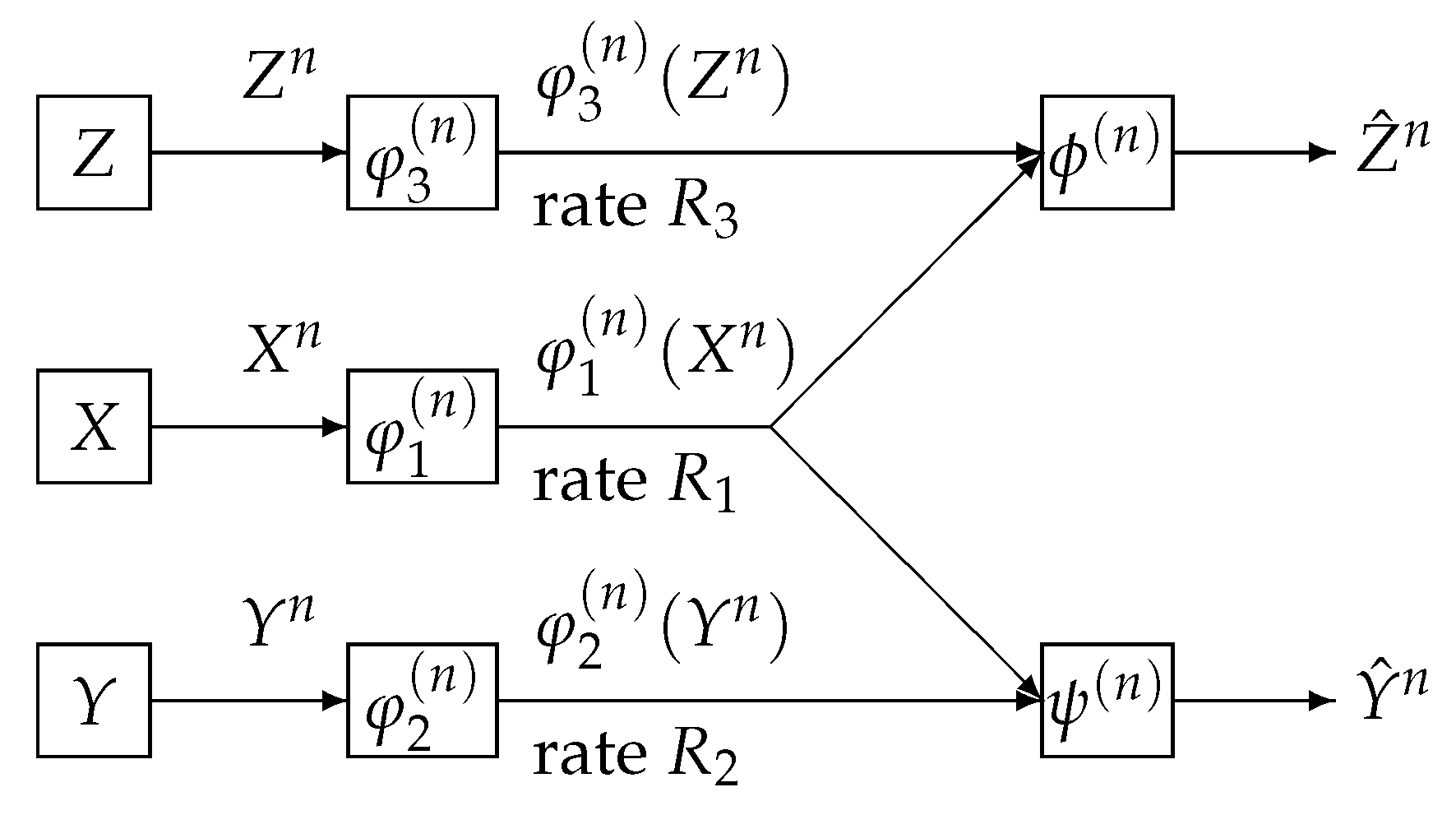
5. One Helper Problem Studied by Wyner
We consider a communication system depicted in
Figure 4. Data sequences
,
, and
, respectively are separately encoded to
,
, and
. The encoded data
and
are sent to the information processing center 1. The encoded data
and
are sent to the information processing center 2. At center 1, the decoder function
observes
to output the estimation
of
. At center 2, the decoder function
observes
to output the estimation
of
. The error probability of decoding is
where
and
.
A rate triple
is
-
achievable if, for any
, there exist a positive integer
and a sequence of three encoders and two decoder functions
such that, for
,
The rate region
is defined by
Furthermore, define
We can show that the two rate regions
,
and
satisfy the following property.
Property 5. - (a)
The regions , , and are closed convex sets of .
- (b)
We setwhich is called the -rate region. Using , can be expressed as
It is well known that
was determined by Wyner. To describe his result, we introduce an auxiliary random variable
U taking values in a finite set
. We assume that the joint distribution of
is
The above condition is equivalent to
. Define the set of probability distribution on
by
Set
We can show that the region
satisfies the following property.
Property 6. - (a)
The region is a closed convex subset of .
- (b)
For any , and any , we have The minimun is attained by . This result implies that Furthermore, the point always belongs to .
The rate region
was determined by Wyner [
2]. His result is the following.
On the strong converse theorem, Csiszár and Körner [
21] obtained the following.
Theorem 5 (Csiszár and Körner [
21]).
For each fixed ε, we have To examine a rate of convergence for the error probability of decoding to tend to one as
for
, we define the following quantity. Set
By time sharing, we have that
Choosing
in (
42), we obtain the following subadditivity property on
:
from which we have that
exists and satisfies the following:
The exponent function
is a convex function of
. In fact, by time sharing, we have that
from which we have that for any
The region
is also a closed convex set. Our main aim is to find an explicit characterization of
. In this paper, we derive an explicit outer bound of
whose section by the plane
coincides with
. We first explain that the region
has another expression using the supporting hyperplane. We define two sets of probability distributions on
by
For
, set
Furthermore, define
Then, we have the following property.
Property 7. - (a)
The bound is sufficient to describe .
- (b)
For every , we have - (c)
For any we have
For
, and for
, define
We next define a function serving as a lower bound of
. For each
, define
Furthermore, set
We can show that the above functions and sets satisfy the following property.
Property 8. - (a)
The cardinality bound in is sufficient to describe the quantity . Furthermore, the cardinality bound in is sufficient to describe the quantity .
- (b)
For any , we have - (c)
For any and any , we have - (d)
Fix any and . We define a probability distribution by Then, for , is twice differentiable. Furthermore, for , we have The second equality implies that is a concave function of .
- (e)
For , defineand set Then, we have . Furthermore, for any , we have - (f)
For every , the condition implies
Since proofs of the results stated in Property 8 are quite parallel with those of the results stated in Property 4, we omit them. Our main result is the following.
Theorem 6. For any , any , and for any satisfying we have It follows from Theorem 6 and Property 8 part d) that, if is outside the capacity region, then the error probability of decoding goes to one exponentially and its exponent is not below . It immediately follows from Theorem 3 that we have the following corollary.
Proof of Theorem 6 is quite parallel with that of Theorem 3. We omit the detail of the proof. From Theorem 6 and Property 8 part e, we can obtain an explicit outer bound of
with an asymptotically vanishing deviation from
. The strong converse theorem established by Csiszár and Körner [
21] immediately follows from this corollary. To describe this outer bound, for
, we set
which serves as an outer bound of
. For each fixed
, we define
by
Step (a) follows from
. Since
as
, we have the smallest positive integer
such that
for
. From Theorem 6 and Property 8 part e, we have the following corollary.
Corollary 5. For each fixed , we choose the above positive integer . Then, for any , we haveThe above result together withyields that for each fixed , we haveThis recovers the strong converse theorem proved by Csiszár and Körner [21]. Proof of this corollary is quite parallel with that of Corollary 2. We omit the detail.


