Exponential Strong Converse for One Helper Source Coding Problem ^†

Abstract

We consider the one helper source coding problem posed and investigated by Ahlswede, Körner and Wyner. Two correlated sources are separately encoded and are sent to a destination where the decoder wishes to decode one of the two sources with an arbitrary small error probability of decoding. In this system, the error probability of decoding goes to one as the source block length n goes to infinity. This implies that we have a strong converse theorem for the one helper source coding problem. In this paper, we provide the much stronger version of this strong converse theorem for the one helper source coding problem. We prove that the error probability of decoding tends to one exponentially and derive an explicit lower bound of this exponent function.

1. Introduction

For single or multi terminal source encoding systems, the converse coding theorems state that, at any data compression rates below the fundamental theoretical limit of the system, the error probability of decoding can not go to zero when the block length n of the codes tends to infinity.

In this paper, we study the one helper source coding problem posed and investigated by Ahlswede, Körner [1] and Wyner [2]. We call the above source coding system (the AKW system). The AKW system is shown in Figure 1.

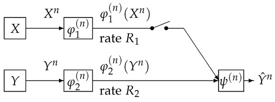
Figure 1. Source encoding with or without side information at the decoder.

In this figure, the AKW system corresponds to the case where the switch is closed. In Figure 1, the sequence $(X^n,Y^n)$ represents independent copies of a pair of dependent random variables $(X,Y)$ which take values in the finite sets $\mathcal{X},\mathcal{Y}$, respectively. We assume that $(X,Y)$ has a probability distribution denoted by $p_{XY}$. For each $i=1,2$, the encoder ${\phi }_i^{(n)}$ outputs a binary sequence which appears at a rate $R_i$ bits per input symbol. The decoder function ${\psi }^{(n)}$ observes ${\phi }_1^{(n)}(X^n)$ and ${\phi }_2^{(n)}(Y^n)$ to output a sequence ${\widehat{Y}}^n:={\psi }^{(n)}({\phi }_1^{(n)}(X^n),{\phi }_2^{(n)}(Y^n))$, which is an estimation of $Y^n$. When the switch is open, it is well known that the minimum transmission rate $R_2$ such that the error probability $P_{\mathrm{e}}^{(n)}:=\mathrm{Pr}\{Y^n\ne {\widehat{Y}}^n\}$ of decoding tends to zero as n tends to infinity is given by $H(Y)$. Csiszár and Longo [3] proved that, if $R_2<H(Y)$, then the correct probability $P_{\mathrm{c}}^{(n)}:=\mathrm{Pr}\{Y^n={\widehat{Y}}^n\}$ of decoding decay exponentially and derived the optimal exponent function. When the switch is open and $R_1>H(X)$, Slepian and Wolf [4] proved that $H(Y|X)$ is the minimum transmission rate $R_2$ such that the error probability $\mathrm{Pr}\{Y^n\ne {\widehat{Y}}^n\}$ of decoding tends to zero as n tends to infinity. Oohama and Han [5] proved that, if $R_2<H(Y|X)$, then the correct probability $P_{\mathrm{c}}^{(n)}:=\mathrm{Pr}\{Y^n={\widehat{Y}}^n\}$ of decoding decay exponentially and derived the optimal exponent function.

In this paper, we consider the strong converse theorem in the case where the switch is closed and $0<R_1<H(X)$. Let ${\mathcal{R}}_{\mathrm{AKW}}(p_{XY})$ be the rate region of the AKW system. This region consists of the rate pair $(R_1,R_2)$ such that the error provability of decoding goes to zero as n tends to infinity. The rate region was determined by Ahlswede, Körner [1] and Wyner [2]. On the converse coding theorem, Ahlswede et al. [6] proved that, if $(R_1,R_2)$ is outside the rate region, then, ${\mathrm{P}}_{\mathrm{c}}^{(n)}$ must tends to zero as n tends to infinity. Gu and Effors [7] examined a speed of convergence for ${\mathrm{P}}_{\mathrm{c}}^{(n)}$ to tend to zero as $n\to \infty$ by carefully checking the proof of Ahlswede et al. [6]. However, they could not obtain a result on an explicit form of the exponent function with respect to the code length n.

Our main results on the strong converse theorem for the AKW system are as follows. For the AKW system, we prove that, if $(R_1,R_2)$ is outside the rate region ${\mathcal{R}}_{\mathrm{AKW}}(p_{XY})$, ${\mathrm{P}}_{\mathrm{c}}^{(n)}$ must go to zero exponentially and derive an explicit lower bound of this exponent. This result corresponds to Theorem 3. As a corollary from this theorem, we obtain the strong converse result, which is stated in Corollary 2. This result states that we have an outer bound with $O(1/\sqrt{n})$ gap from the rate region ${\mathcal{R}}_{\mathrm{AKW}}(p_{XY})$.

To derive our result, we use a new method called the recursive method. This method, which is a new method introduced by the author, includes a certain recursive algorithm for a single letterization of exponent functions. In a standard argument of proving converse coding theorems, single letterization methods based on the chain rule of the entropy functions are used. In general, the functions representing multi letter characterizations of exponent functions do not have the chain rule property. In such cases, the recursive method is quite useful for deriving single letterized bounds. The recursive method is a general powerful tool to prove strong converse theorems for several coding problems in information theory. In fact, the recursive method plays important roles in deriving exponential strong converse exponent for communication systems treated in [8,9,10,11,12].

On the strong converse theorem for the one helper source coding problem, we have two recent other works [13,14]. The above two works proved the strong converse theorem using different methods from our method. In [13], Watanabe found a relationship between the AKW system and the Gray–Wyner network. Using this relationship and the second order rate region for the Gray–Wyner network obtained by him [15], Watanabe established the strong converse theorem for the AKW system. In [14], Liu et al. introduced a new method to derive sharp strong converse bounds via a reverse hypercontractivity. Using this method, they obtained an outer bound of the rate region for the AKW system with $O(1/\sqrt{n})$ gap from the rate region. Furthermore, in [14], an extension of the AKW system to the case of Gaussian source and quadratic distortion is investigated, obtaining an outer bound with $O(1/\sqrt{n})$ gap from the rate distortion region for the extended source coding system. In his resent paper [16], Liu showed a lower bound (converse) on the dispersion of AWK as the variance of the linear combination of information densities.

The strong converse theorems seem to be regarded just as a mathematical problem and have been investigated mainly from theoretical interest. Recently, Watanabe and Oohama [17] have found an interesting security problem, which has a close connection with the strong converse theorem for the AKW system. Furthermore, Oohama and Santoso [18] and Santoso and Oohama [19] clarify that the exponential strong converse theorem obtained by this paper plays an essential role in deriving a strong sufficient secure condition for the privacy amplification in their new theoritical model of side channel attacks to the Shannon chipher systems. From the above two cases, we expect that exponential strong converse theorems for multiterminal source networks will serve as a strong tool to several information theoretical security problems.

2. Problem Formulation

Let $\mathcal{X}$ and $\mathcal{Y}$ be finite sets and ${\left\{(X_t,Y_t)\right\}}_{t=1}^{\infty }$ be a stationary discrete memoryless source. For each $t=1,2,\cdots$, the random pair $(X_t,Y_t)$ takes values in $\mathcal{X}\times \mathcal{Y}$, and has a probability distribution

$$p_{XY}={\left\{p_{XY}(x,y)\right\}}_{(x,y)\in \mathcal{X}\times \mathcal{Y}}.$$

We write n independent copies of ${\left\{X_t\right\}}_{t=1}^{\infty }$ and ${\left\{Y_t\right\}}_{t=1}^{\infty }$, respectively as

$$X^n=X_1,X_2,\cdots ,X_n\mathrm{and}{Y}^n=Y_1,Y_2,\cdots ,Y_n.$$

We consider a communication system depicted in Figure 2. This communication system corresponds to the case where the switch is closed in Figure 1. Data sequences $X^n$ and $Y^n$ are separately encoded to ${\phi }_1^{(n)}(X^n)$ and ${\phi }_2^{(n)}(Y^n)$ and those are sent to the information processing center. At the center, the decoder function ${\psi }^{(n)}$ observes $({\phi }_1^{(n)}(X^n),{\phi }_2^{(n)}(Y^n))$ to output the estimation ${\widehat{Y}}^n$ of $Y^n$. The encoder functions ${\phi }_1^{(n)}$ and ${\phi }_2^{(n)}$ are defined by

$$\left.\begin{array}{c}{\phi }_1^{(n)}:{\mathcal{X}}^n\to {\mathcal{M}}_1=\left\{1,2,\cdots ,M_1\right\}\hfill \\ {\phi }_2^{(n)}:{\mathcal{Y}}^n\to {\mathcal{M}}_2=\left\{1,2,\cdots ,M_2\right\}\hfill \end{array}\right\},$$

(1)

where for each $i=1,2$, $\parallel {\phi }_i^{(n)}\parallel$$(=M_i)$ stands for the range of cardinality of ${\phi }_i^{(n)}$. The decoder function ${\psi }^{(n)}$ is defined by

$${\psi }^{(n)}:{\mathcal{M}}_1\times {\mathcal{M}}_2\to {\mathcal{Y}}^n.$$

(2)

The error probability of decoding is

$${\mathrm{P}}_{\mathrm{e}}^{(n)}({\phi }_1^{(n)},{\phi }_2^{(n)},{\psi }^{(n)})=Pr\left\{{\widehat{Y}}^n\ne Y^n\right\},$$

(3)

where ${\widehat{Y}}^n={\psi }^{(n)}({\phi }_1^{(n)}(X^n),{\phi }_2^{(n)}(Y^n))$. A rate pair $(R_1,R_2)$ is $\epsilon$-achievable if, for any $\delta >0$, there exists a positive integer $n_0=n_0(\epsilon ,\delta )$ and a sequence of triples $\{({\phi }_1^{(n)},$${\phi }_2^{(n)},$ ${\psi }^{(n)}{)\}}_{n\ge n_0}$ such that, for $n\ge n_0$,

$$\begin{array}{c}\frac{1}{n}log\parallel {\phi }_i^{(n)}\parallel \le R_i+\delta \mathrm{for}i=1,2,{\mathrm{P}}_{\mathrm{e}}^{(n)}({\phi }_1^{(n)},{\phi }_2^{(n)},{\psi }^{(n)})\le \epsilon .\hfill \end{array}$$

For $\epsilon \in (0,1)$, the rate region ${\mathcal{R}}_{\mathrm{AKW}}(\epsilon |p_{XY})$ is defined by

$$\begin{array}{c}{\mathcal{R}}_{\mathrm{AKW}}(\epsilon |p_{XY}):=\left\{(R_1,R_2):(R_1,R_2)\mathrm{is}\epsilon -\mathrm{achievable}\mathrm{for}{p}_{XY}\right\}.\hfill \end{array}$$

Furthermore, define

$${\mathcal{R}}_{\mathrm{AKW}}(p_{XY}):=\bigcap _{\epsilon \in (0,1)}{\mathcal{R}}_{\mathrm{AKW}}(\epsilon |p_{XY}).$$

We can show that the two rate regions ${\mathcal{R}}_{\mathrm{AKW}}(\epsilon |$$p_{XY})$, $\epsilon \in (0,1)$ and ${\mathcal{R}}_{\mathrm{AKW}}(p_{XY})$ satisfy the following property.

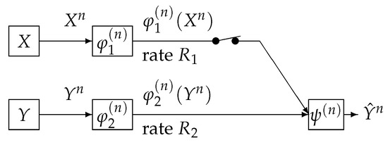
Figure 2. One helper source coding system [20].

Property 1.

(a) 

The regions ${\mathcal{R}}_{\mathrm{AKW}}(\epsilon |p_{XY})$, $\epsilon \in (0,1)$, and ${\mathcal{R}}_{\mathrm{AKW}}($$p_{XY})$ are closed convex sets of ${\mathbb{R}}_{+}^2$, where

$$\begin{array}{cc}\hfill {\mathbb{R}}_{+}^2& :=\{(R_1,R_2):R_1\ge 0,R_2\ge 0\}.\hfill \end{array}$$

(b) 

${\mathcal{R}}_{\mathrm{AKW}}(\epsilon |p_{XY})$ has another form using $(n,\epsilon )$-rate region ${\mathcal{R}}_{\mathrm{AKW}}(n,\epsilon |p_{XY})$, the definition of which is as follows. We set

$$\begin{array}{c}{\mathcal{R}}_{\mathrm{AKW}}(n,\epsilon |p_{XY})=\{(R_1,R_2):Thereexists({\phi }_1^{(n)},{\phi }_2^{(n)},{\psi }^{(n)})suchthat\hfill \\ \frac{1}{n}log\left|\right|{\phi }_i^{(n)}\left|\right|\le R_i,i=1,2,{\mathrm{P}}_{\mathrm{e}}^{(n)}({\phi }_1^{(n)},{\phi }_2^{(n)},{\psi }^{(n)})\le \epsilon \}.\hfill \end{array}$$

Using ${\mathcal{R}}_{\mathrm{AKW}}(n,$$\epsilon |p_{XY})$, ${\mathcal{R}}_{\mathrm{AKW}}(\epsilon |p_{XY})$ can be expressed as

$$\begin{array}{cc}\hfill {\mathcal{R}}_{\mathrm{AKW}}(\epsilon |p_{XY})& =\mathrm{cl}\left(\bigcup _{m\ge 1}\bigcap _{n\ge m}{\mathcal{R}}_{\mathrm{AKW}}(n,\epsilon |p_{XY})\right).\hfill \end{array}$$

Proof of this property is given in Appendix A. It is well known that ${\mathcal{R}}_{\mathrm{AKW}}(p_{XY})$ was determined by Ahlswede, Körner and Wyner. To describe their result, we introduce an auxiliary random variable U taking values in a finite set $\mathcal{U}$. We assume that the joint distribution of $(U,X,Y)$ is

$$p_{UXY}(u,x,y)=p_U(u)p_{X|U}(x|u)p_{Y|X}(y|x).$$

The above condition is equivalent to $U\leftrightarrow X\leftrightarrow Y$. Define the set of probability distribution $p=p_{UXY}$ by

$$\begin{array}{c}\mathcal{P}(p_{XY}):=\{p_{UXY}:\left|\mathcal{U}\right|\le \left|\mathcal{X}\right|+1,U\leftrightarrow X\leftrightarrow Y\}.\hfill \end{array}$$

Set

$$\begin{array}{cc}\hfill \mathcal{R}(p)& :=\begin{array}{c}\{(R_1,R_2):R_1,R_2\ge 0\begin{array}{ccc}\hfill R_1& \ge & I_p(X;U),R_2\ge H_p(Y|U)\},\hfill \end{array}\hfill \end{array}\hfill \\ \hfill \mathcal{R}(p_{XY})& :=\bigcup _{p\in \mathcal{P}(p_{XY})}\mathcal{R}(p).\hfill \end{array}$$

We can show that the region $\mathcal{R}(p_{XY})$ satisfies the following property.

Property 2.

(a) 

The region $\mathcal{R}(p_{XY})$ is a closed convex subset of ${\mathbb{R}}_{+}^2$.

(b) 

For any $p_{XY}$, we have

$$\underset{(R_1,R_2)\in \mathcal{R}(p_{XY})}{min}(R_1+R_2)=H_p(Y).$$

(4)

The minimum is attained by $(R_1,R_2)=(0,H_p(Y))$. This result implies that

$$\begin{array}{c}\mathcal{R}(p_{XY})\subseteq \{(R_1,R_2):R_1+R_2\ge H_p(Y)\}\cap {\mathbb{R}}_{+}^2.\hfill \end{array}$$

Furthermore, the point $(0,H_p(Y))$ always belongs to $\mathcal{R}(p_{XY})$.

Property 2 part a is a well known property. Proof of Property 2 part b is easy. Proofs of Property 2 parts a and b are omitted. A typical shape of the rate region $\mathcal{R}(p_{XY})$ is shown in Figure 3.

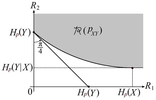
Figure 3. A typical shape of $\mathcal{R}(p_{XY})$.

The rate region ${\mathcal{R}}_{\mathrm{AKW}}(p_{XY})$ was determined by Ahlswede and Körner [1] and Wyner [2]. Their results are the following.

Theorem 1

(Ahlswede, Körner [1] and Wyner [2]).

$$\begin{array}{c}{\mathcal{R}}_{\mathrm{AKW}}(p_{XY})=\mathcal{R}(p_{XY}).\hfill \end{array}$$

On the converse coding theorem, Ahlswede et al. [6] obtained the following.

Theorem 2

(Ahlswede et al. [6]). For each fixed ε$\in (0,1)$, we have

$$\begin{array}{c}{\mathcal{R}}_{\mathrm{AKW}}(\epsilon |p_{XY})=\mathcal{R}(p_{XY}).\hfill \end{array}$$

Gu and Effors [7] examined a speed of convergence for ${\mathrm{P}}_{\mathrm{e}}^{(n)}$ to tend to 1 as $n\to \infty$ by carefully checking the proof of Ahlswede et al. [6]. However, they could not obtain a result on an explicit form of the exponent function with respect to the code length n.

Our aim is to find an explicit form of the exponent function for the error probability of decoding to tend to one as $n\to \infty$ when $(R_1,R_2)\notin {\mathcal{R}}_{\mathrm{AKW}}(p_{XY})$. To examine this quantity, we define the following quantity. Set

$$\begin{array}{c}{\mathrm{P}}_{\mathrm{c}}^{(n)}({\phi }_1^{(n)},{\phi }_2^{(n)},{\psi }^{(n)}):=1-{\mathrm{P}}_{\mathrm{e}}^{(n)}({\phi }_1^{(n)},{\phi }_2^{(n)},{\psi }^{(n)}),\hfill \\ G^{(n)}(R_1,R_2|p_{XY}):=\underset{\genfrac{}{}{0pt}{}{({\phi }_1^{(n)},{\phi }_2^{(n)},{\psi }^{(n)}):}{(1/n)log\parallel {\phi }_i^{(n)}\parallel \le R_i,i=1,2}}{min}\left(-\frac{1}{n}\right)log{\mathrm{P}}_{\mathrm{c}}^{(n)}({\phi }_1^{(n)},{\phi }_2^{(n)},{\psi }^{(n)}).\hfill \\ G(R_1,R_2|p_{XY}):=\underset{n\to \infty }{lim}{G}^{(n)}(R_1,R_2|p_{XY}),\hfill \\ \mathcal{G}(p_{XY}):=\{(R_1,R_2,G):G\ge G(R_1,R_2|p_{XY})\}.\hfill \end{array}$$

By time sharing, we have that

$$\begin{array}{c}{G}^{(n+m)}\left(\left.\frac{n{R}_1+m{R}_1^{\prime }}{n+m},\frac{n{R}_2+m{R}_2^{\prime }}{n+m}\right|p_{XY}\right)\le \frac{n{G}^{(n)}(R_1,R_2|p_{XY})+m{G}^{(m)}(R_1^{\prime },R_2^{\prime }|p_{XY})}{n+m}.\hfill \end{array}$$

(5)

Choosing $R=R^{\prime }$ in the inequality (5), we obtain the following subadditivity property on $\{G^{(n)}(R_1,R_2|p_{XY})$${\}}_{n\ge 1}$:

$$\begin{array}{c}{G}^{(n+m)}(R_1,R_2|p_{XY})\le \frac{n{G}^{(n)}(R_1,R_2|p_{XY})+m{G}^{(m)}(R_1,R_2|p_{XY})}{n+m},\hfill \end{array}$$

from which this, and Fekete’s subadditive lemma, we have that $G^{(n)}(R_1,R_2|p_{XY})$ exists and satisfies the following:

$$\begin{array}{c}\underset{n\to \infty }{lim}{G}^{(n)}(R_1,R_2|p_{XY})=\underset{n\ge 1}{inf}{G}^{(n)}(R_1,R_2|p_{XY}).\hfill \end{array}$$

The exponent function $G(R_1,R_2|p_{XY})$ is a convex function of $(R_1,R_2)$. In fact, from the inequality (5), we have that for any $\alpha \in [0,1]$

$$\begin{array}{c}G(\alpha R_1+\overline{\alpha }{R}_1^{\prime },\alpha R_2+\overline{\alpha }{R}_2^{\prime }|p_{XY})\le \alpha G(R_1,R_2|p_{XY})+\overline{\alpha }G(R_1^{\prime },R_2^{\prime }|p_{XY}).\hfill \end{array}$$

The region $\mathcal{G}(p_{XY})$ is also a closed convex set. Our main aim is to find an explicit characterization of $\mathcal{G}(p_{XY})$. In this paper, we derive an explicit outer bound of $\mathcal{G}$$(p_{XY})$ whose section by the plane $G=0$ coincides with ${\mathcal{R}}_{\mathrm{AKW}}(p_{XY})$.

3. Main Results

In this section, we state our main result. We first explain that the region $\mathcal{R}(p_{XY})$ can be expressed with a family of supporting hyperplanes. To describe this result, we define a set of probability distributions on $\mathcal{U}$$\times \mathcal{X}$$\times \mathcal{Y}$ by

$$\begin{array}{cc}\hfill {\mathcal{P}}_{\mathrm{sh}}(p_{XY})& :=\{p=p_{UXY}:|\mathcal{U}|\le |\mathcal{X}|,U\leftrightarrow X\leftrightarrow Y\}.\hfill \end{array}$$

For $\mu \ge 0$, define

$$\begin{array}{c}{R}^{(\mu )}(p_{XY}):=\underset{p\in {\mathcal{P}}_{\mathrm{sh}}(p_{XY})}{min}\left\{\mu I_p(X;U)+\overline{\mu }{H}_p(Y|U)\right\}.\hfill \end{array}$$

Furthermore, define

$$\begin{array}{c}{\mathcal{R}}_{\mathrm{sh}}(p_{XY}):=\bigcap _{\mu \in [0,1]}\{(R_1,R_2):\begin{array}{c}\mu R_1+\overline{\mu }{R}_2\ge R^{(\mu )}(p_{XY})\}.\hfill \end{array}\hfill \end{array}$$

Then, we have the following property.

Property 3.

(a) 

The bound $\left|\mathcal{U}\right|\le \left|\mathcal{X}\right|$ is sufficient to describe $R^{(\mu )}($$p_{XY})$.

(b) 

For every $\mu \in [0,1]$, we have

$$\begin{array}{c}\underset{(R_1,R_2)\in \mathcal{R}(p_{XY})}{min}\{\mu R_1+\overline{\mu }{R}_2\}=R^{(\mu )}(p_{XY}).\hfill \end{array}$$

(6)

(c) 

For any $p_{XY},$ we have

$${\mathcal{R}}_{\mathrm{sh}}(p_{XY})=\mathcal{R}(p_{XY}).$$

(7)

Property 3 part a is stated as Lemma A1 in Appendix B. Proof of this lemma is given in this appendix. Proofs of Property 3 parts b and c are given in Appendix C. Set

$$\begin{array}{cc}\hfill \mathcal{Q}(p_{Y|X})& :=\{q=q_{UXY}:|\mathcal{U}|\le |\mathcal{X}|,U\leftrightarrow X\leftrightarrow Y,p_{Y|X}=q_{Y|X}\}.\hfill \end{array}$$

For $(\mu ,\alpha )\in {[0,1]}^2$, and for $q=q_{UXY}\in \mathcal{Q}(p_{Y|X})$, define

$$\begin{array}{c}{\omega }_{q|p_X}^{(\mu ,\alpha )}(x,y|u):=\overline{\alpha }log\frac{q_X(x)}{p_X(x)}+\alpha \left[\mu log\frac{q_{X|U}(x|u)}{p_X(x)}\right.\left.+\overline{\mu }log\frac{1}{q_{Y|U}(y|u)}\right],\hfill \\ f_{q|p_X}^{(\mu ,\alpha )}(x,y|u):=exp\left\{-{\omega }_{q|p_X}^{(\mu ,\alpha )}(x,y|u)\right\},\hfill \\ {\Omega }^{(\mu ,\alpha )}(q|p_X):=-log{\mathrm{E}}_q\left[exp\left\{-{\omega }_{q|p_X}^{(\mu ,\alpha )}(X,Y|U)\right\}\right],{\Omega }^{(\mu ,\alpha )}(p_{XY}):=\underset{\genfrac{}{}{0pt}{}{}{q\in \mathcal{Q}(p_{Y|X})}}{min}{\Omega }^{(\mu ,\alpha )}(q|p_X),\hfill \\ F^{(\mu ,\alpha )}(\mu R_1+\overline{\mu }{R}_2|p_{XY}):=\frac{{\Omega }^{(\mu ,\alpha )}(p_{XY})-\alpha (\mu R_1+\overline{\mu }{R}_2)}{2+\alpha \overline{\mu }},\hfill \\ F(R_1,R_2|p_{XY}):=\underset{(\mu ,\alpha )\in {[0,1]}^2}{sup}{F}^{(\mu ,\alpha )}(\mu R_1+\overline{\mu }{R}_2|p_{XY}).\hfill \end{array}$$

We next define a function serving as a lower bound of $F(R_1,R_2|p_{XY})$. For $\lambda \ge 0$ and for $p_{UXY}\in {\mathcal{P}}_{\mathrm{sh}}(p_{XY})$, define

$$\begin{array}{c}{\tilde{\omega }}_p^{(\mu )}(x,y|u):=\mu log\frac{p_{X|U}(x|u)}{p_X(x)}+\overline{\mu }log\frac{1}{p_{Y|U}(y|u)},\hfill \\ {\tilde{\Omega }}^{(\mu ,\lambda )}(p):=-log{\mathrm{E}}_p\left[exp\left\{-\lambda {\tilde{\omega }}_p^{(\mu )}(X,Y|U)\right\}\right],{\tilde{\Omega }}^{(\mu ,\lambda )}(p_{XY}):=\underset{\genfrac{}{}{0pt}{}{}{p\in {\mathcal{P}}_{\mathrm{sh}}(p_{XY})}}{min}{\tilde{\Omega }}^{(\mu ,\lambda )}(p).\hfill \end{array}$$

Furthermore, set

$$\begin{array}{c}{\underline{F}}^{(\mu ,\lambda )}(\mu R_1+\overline{\mu }{R}_2|p_{XY}):=\frac{{\tilde{\Omega }}^{(\mu ,\lambda )}(p_{XY})-\lambda (\mu R_1+\overline{\mu }{R}_2)}{2+\lambda (5-\mu )},\hfill \\ \underline{F}(R_1,R_2|p_{XY}):=\underset{\lambda \ge 0,\mu \in [0,1]}{sup}{\underline{F}}^{(\mu ,\lambda )}(\mu R_1+\overline{\mu }{R}_2|p_{XY}).\hfill \end{array}$$

We can show that the above functions satisfy the following property.

Property 4.

(a) 

The cardinality bound $\left|\mathcal{U}\right|\le \left|\mathcal{X}\right|$ in $\mathcal{Q}(p_{Y|X})$ is sufficient to describe the quantity ${\Omega }^{(\mu ,\alpha )}(p_{XY})$. Furthermore, the cardinality bound $\left|\mathcal{U}\right|\le \left|\mathcal{X}\right|$ in ${\mathcal{P}}_{\mathrm{sh}}(p_{XY})$ is sufficient to describe the quantity ${\tilde{\Omega }}^{(\mu ,\lambda )}(p_{XY})$.

(b) 

For any $R_1,R_2\ge 0$, we have

$$\begin{array}{c}\hfill F(R_1,R_2|p_{XY})\ge \underline{F}(R_1,R_2|p_{XY}).\end{array}$$

(c) 

For any $p=p_{UXY}\in {\mathcal{P}}_{\mathrm{sh}}(p_{XY})$ and any $(\mu ,\lambda$${)\in [0,1]}^2$, we have

$$0\le {\tilde{\Omega }}^{(\mu ,\lambda )}(p)\le \mu log\left|\mathcal{X}\right|+\overline{\mu }log\left|\mathcal{Y}\right|.$$

(8)

(d) 

Fix any $p=p_{UXY}\in {\mathcal{P}}_{\mathrm{sh}}(p_{XY})$ and $\mu \in [0,1]$. For $\lambda \in [0,1]$, we define a probability distribution $p^{(\lambda )}=p_{UXY}^{(\lambda )}$ by

$$\begin{array}{c}{p}^{(\lambda )}(u,x,y):=\frac{p(u,x,y)exp\left\{-\lambda {\tilde{\omega }}_p^{(\mu )}(x,y|u)\right\}}{{\mathrm{E}}_p\left[exp\left\{-\lambda {\tilde{\omega }}_p^{(\mu )}(X,Y|U)\right\}\right]}.\hfill \end{array}$$

Then, for $\lambda \in [0,1/2]$, ${\tilde{\Omega }}^{(\mu ,\lambda )}(p)$ is twice differentiable. Furthermore, for $\lambda \in [0,1/2]$, we have

$$\begin{array}{c}\frac{\mathrm{d}}{\mathrm{d}\lambda }{\tilde{\Omega }}^{(\mu ,\lambda )}(p)={\mathrm{E}}_{p^{(\lambda )}}\left[{\tilde{\omega }}_p^{(\mu )}(X,Y|U)\right],\frac{{\mathrm{d}}^2}{\mathrm{d}{\lambda }^2}{\tilde{\Omega }}^{(\mu ,\lambda )}(p)=-{\mathrm{Var}}_{p^{(\lambda )}}\left[{\tilde{\omega }}_p^{(\mu )}(X,Y|U)\right].\hfill \end{array}$$

The second equality implies that ${\tilde{\Omega }}^{(\mu ,\lambda )}(p$$|p_{XY})$ is a concave function of $\lambda \in [0,1/2]$.

(e) 

For every $(\mu ,\lambda )\in [0,1]\times [0,1/2]$, define

$$\begin{array}{c}{\rho }^{(\mu ,\lambda )}(p_{XY}):=\underset{\genfrac{}{}{0pt}{}{(\nu ,p)\in [0,\lambda ]\times {\mathcal{P}}_{\mathrm{sh}}(p_{XY}):}{{\tilde{\Omega }}^{(\mu ,\lambda )}(p)={\tilde{\Omega }}^{(\mu ,\lambda )}(p_{XY})}}{max}{\mathrm{Var}}_{p^{(\nu )}}\left[{\tilde{\omega }}_p^{(\mu )}(X,Y|U)\right],\hfill \end{array}$$

and set

$$\begin{array}{c}\rho =\rho (p_{XY}):=\underset{(\mu ,\lambda )\in [0,1]\times [0,1/2]}{max}{\rho }^{(\mu ,\lambda )}(p_{XY}).\hfill \end{array}$$

Then, we have $\rho (p_{XY})<\infty .$ Furthermore, for any $(\mu ,\lambda )\in [0,1]\times [0,1/2]$, we have

$${\tilde{\Omega }}^{(\mu ,\lambda )}(p_{XY})\ge \lambda R^{(\mu )}(p_{XY})-\frac{{\lambda }^2}{2}\rho (p_{XY}).$$

(9)

(f) 

For every $\tau \in (0,(1/2)\rho (p_{XY}))$, the condition $(R_1+\tau ,$$R_2+\tau )\notin \mathcal{R}(p_{XY})$ implies

$$\underline{F}(R_1,R_2|p_{XY})>\frac{\rho (p_{XY})}{4}·g^2\left(\frac{\tau }{\rho (p_{XY})}\right)>0,$$

where g is the inverse function of $\vartheta (a):=a+(5/4)a^2,a\ge 0$.

Property 3 part a is stated as Lemma A2 in Appendix B. Proof of this lemma is given in this appendix. Proof of Property 4 part b is given in Appendix D. Proofs of Property 4 parts c, d, e, and f are given in Appendix E.

Our main result is the following.

Theorem 3.

For any $R_1,R_2\ge 0$, any $p_{XY}$, and for any $({\phi }_1^{(n)},$ ${\phi }_1^{(n)},$ ${\psi }^{(n)})$ satisfying $(1/n)log\left|\right|{\phi }_i^{(n)}\left|\right|\le R_i,i=1,2,$ we have

$${\mathrm{P}}_{\mathrm{c}}^{(n)}({\phi }_1^{(n)},{\phi }_2^{(n)},{\psi }^{(n)})\le 5exp\left\{-nF(R_1,R_2|p_{XY})\right\}.$$

(10)

It can be seen from Property 4 parts b and f that $F(R_1,R_2|p_{XY})$ is strictly positive if $(R_1,R_2)$ is outside the rate region $\mathcal{R}(p_{XY})$. Hence, by Theorem 3, we have that, if $(R_1,R_2)$ is outside the rate region, then the error probability of decoding goes to one exponentially and its exponent is not below $F(R_1,R_2|p_{XY})$. It immediately follows from Theorem 3 that we have the following corollary.

Corollary 1.

$$\begin{array}{c}G(R_1,R_2|p_{XY})\ge F(R_1,R_2|p_{XY}),\hfill \\ \mathcal{G}(p_{XY})\subseteq \overline{\mathcal{G}}(p_{XY})=\left\{(R_1,R_2,G):G\ge F(R_1,R_2|p_{XY})\right\}.\hfill \end{array}$$

Proof of Theorem 3 will be given in the next section. The exponent function at rates outside the rate region was derived by Oohama and Han [5] for the separate source coding problem for correlated sources [4]. The techniques used by them is a method of types [21], which is not useful to prove Theorem 3. Some novel techniques based on the information spectrum method introduced by Han [22] are necessary to prove this theorem.

From Theorem 3 and Property 4 part e, we can obtain an explicit outer bound of ${\mathcal{R}}_{\mathrm{AKW}}(\epsilon |p_{XY})$ with an asymptotically vanishing deviation from ${\mathcal{R}}_{\mathrm{AKW}}(p_{XY})$$=\mathcal{R}(p_{XY})$. The strong converse theorem established by Ahlswede et al. [6] immediately follows from this corollary. To describe this outer bound, for $\kappa >0$, we set

$$\mathcal{R}(p_{XY})-\kappa (1,1):=\{(R_1-\kappa ,R_2-\kappa ):(R_1,R_2)\in \mathcal{R}(p_{XY})\},$$

which serves as an outer bound of $\mathcal{R}(p_{XY})$. For each fixed $\epsilon \in (0,1)$, we define ${\kappa }_n$$={\kappa }_n(\epsilon ,\rho (p_{XY}))$ by

$$\begin{array}{ccc}\hfill {\kappa }_n& :=& \rho (p_{XY})\vartheta \left(\sqrt{\frac{4}{n\rho (p_{XY})}log\left(\frac{5}{1-\epsilon }\right)}\right)\hfill \\ & \stackrel{(\mathrm{a})}{=}& 2\sqrt{\frac{\rho (p_{XY})}{n}log\left(\frac{5}{1-\epsilon }\right)}+\frac{5}{n}log\left(\frac{5}{1-\epsilon }\right).\hfill \end{array}$$

(11)

Step (a) follows from $\vartheta (a)=a+(5/4)a^2$. Since ${\kappa }_n\to 0$ as $n\to \infty$, we have the smallest positive integer $n_0=n_0(\epsilon ,\rho (p_{XY}))$ such that ${\kappa }_n\le (1/2)\rho (p_{XY})$ for $n\ge n_0$. From Theorem 3 and Property 4 part e, we have the following corollary.

Corollary 2.

For each fixed ε$\in (0,1)$, we choose the above positive integer $n_0=$$n_0(\epsilon ,\rho (p_{XY}))$. Then, for any $n\ge n_0$, we have

$$\begin{array}{c}\hfill {\mathcal{R}}_{\mathrm{AKW}}(n,\epsilon |p_{XY})\subseteq \mathcal{R}(p_{XY})-{\kappa }_n(1,1).\end{array}$$

The above result together with

$$\begin{array}{cc}\hfill {\mathcal{R}}_{\mathrm{AKW}}(\epsilon |p_{XY})& =\mathrm{cl}\left(\bigcup _{m\ge 1}\bigcap _{n\ge m}{\mathcal{R}}_{\mathrm{AKW}}(n,\epsilon |p_{XY})\right)\hfill \end{array}$$

yields that, for each fixed $\epsilon \in (0,1)$, we have

$$\begin{array}{c}{\mathcal{R}}_{\mathrm{AKW}}(\epsilon |p_{XY})={\mathcal{R}}_{\mathrm{AKW}}(p_{XY})=\mathcal{R}(p_{XY}).\hfill \end{array}$$

This recovers the strong converse theorem proved by Ahlswede et al. [6].

Proof of this corollary will be given in the next section.

4. Proof of the Main Result

Let $(X^n,Y^n)$ be a pair of random variables from the information source. We set $S={\phi }_1^{(n)}(X^n)$. Joint distribution $p_{S{X}^n{Y}^n}$ of $(S,X^n,Y^n)$ is given by

$$\begin{array}{c}{p}_{S{X}^n{Y}^n}(s,x^n,y^n)=p_{S|X^n}(s|x^n)\prod _{t=1}^n{p}_{X_t{Y}_t}(x_t,y_t).\hfill \end{array}$$

It is obvious that $S\leftrightarrow X^n\leftrightarrow Y^n$. Then, we have the following lemma, which is well known as a single shot infomation spectrum bound.

Lemma 1.

For any $\eta >0$ and for any $({\phi }_1^{(n)}$, ${\phi }_2^{(n)},{\psi }^{(n)})$ satisfying $(1/n)log\left|\right|{\phi }_i^{(n)}\left|\right|\le R_i,i=1,2,$ we have

$$\begin{array}{cc}\hfill {\mathrm{P}}_{\mathrm{c}}^{(n)}({\phi }_1^{(n)},{\phi }_2^{(n)},{\psi }^{(n)})\le p_{S{X}^n{Y}^n}\{& {\displaystyle 0\ge \frac{1}{n}log\frac{{\widehat{q}}_{{S{X}^{n}Y}^n}(S,X^n,Y^n)}{p_{S{X}^n{Y}^n}(S,X^n,Y^n)}-\eta ,}\hfill \end{array}$$

(12)

$$\begin{array}{c}{\displaystyle 0\ge \frac{1}{n}log\frac{Q_{X^n}(X^n)}{p_{X^n}(X^n)}-\eta ,}\hfill \end{array}$$

(13)

$$\begin{array}{c}{\displaystyle R_1\ge \frac{1}{n}log\frac{{\tilde{Q}}_{X^n|S}(X^n|S)}{p_{X^n}(X^n)}-\eta ,}\hfill \end{array}$$

(14)

$$\begin{array}{c}{\displaystyle R_2\ge \left.\frac{1}{n}log\frac{1}{p_{Y^n|S}(Y^n|S)}-\eta \right\}+4{\mathrm{e}}^{-n\eta }.}\hfill \end{array}$$

(15)

The probability distributions appearing in the three inequalities (12), (13), and (14) in the right members of (15) have a property that we can select them as arbitrary. In (12), we can choose any probability distribution ${\widehat{q}}_{S{X}^n{Y}^n}$ on $\mathcal{S}$$\times {\mathcal{X}}^n$$\times {\mathcal{Y}}^n$. In (13), we can choose any distribution $Q_{X^n}$ on ${\mathcal{X}}^n$. In (14), we can choose any stochastic matrix ${\tilde{Q}}_{X^n|U^n}$: ${\mathcal{X}}^n$ $\to {\mathcal{U}}^n$.

This lemma can be proved by a standard argument in the information spectrum method [22]. The detail of the proof is given in Appendix F. Next, we single letterize the four information spectrum quantities inside the first term in the right members of (15) in Lemma 1 to obtain the following lemma.

Lemma 2.

For any $\eta >0$ and for any $({\phi }_1^{(n)}$, ${\phi }_2^{(n)},{\psi }^{(n)})$ satisfying $(1/n)log\left|\right|{\phi }_i^{(n)}\left|\right|\le R_i,i=1,2,$ we have

$$\begin{array}{c}{\mathrm{P}}_{\mathrm{c}}^{(n)}({\phi }_1^{(n)},{\phi }_2^{(n)},{\psi }^{(n)})\le p_{S{X}^n{Y}^n}\left\{0\ge \frac{1}{n}\sum _{t=1}^{n}log\frac{Q_{X_t}(X_t)}{p_{X_t}(X_t)}-\eta ,\right.\hfill \end{array}$$

(16)

$$\begin{array}{c}{R}_1\ge \frac{1}{n}\sum _{t=1}^{n}log\frac{{\tilde{Q}}_{X_t|S{X}^{t-1}}(X_t|S,X^{t-1})}{p_{X_t}(X_t)}-\eta ,\hfill \end{array}$$

(17)

$$\begin{array}{c}{R}_2\ge \left.\frac{1}{n}\sum _{t=1}^{n}log\frac{1}{p_{Y_t|S{X}^{t-1}{Y}^{t-1}}(Y_t|S,X^{t-1},Y^{t-1})}-2\eta \right\}+4{\mathrm{e}}^{-n\eta },\hfill \end{array}$$

where for each $t=1,2,\cdots ,n$, the probability distribution $Q_{X_t}$ on $\mathcal{X}$ appearing in (16) and the stochastic matrix ${\tilde{Q}}_{X_t|S{X}^{t-1}}:$${\mathcal{M}}_1\times {\mathcal{X}}^{t-1}$$\to \mathcal{X}$ appearing in (17) have a property that we can choose their values arbitrary.

Proof. 

In (12) in Lemma 1, we choose ${\widehat{q}}_{S{X}^n{Y}^n}$ having the form

$$\begin{array}{c}{\widehat{q}}_{S{X}^n{Y}^n}(S,X^n,Y^n)=p_S(S)\prod _{t=1}^n\left\{p_{X_t|S{X}^{t-1}{Y}^t}(X_t|S,X^{t-1},Y^t)p_{Y_t|S{Y}^{t-1}}(Y_t|S,Y^{t-1})\right\}.\hfill \end{array}$$

In (13) in Lemma 1, we choose $Q_{X^n}$ having the form

$$Q_{X^n}(X^n)=\prod _{t=1}^n{Q}_{X_t}(X_t).$$

We further note that

$$\begin{array}{c}\frac{{\tilde{Q}}_{X^n|S}(X^n|S)}{p_{X^n}(X^n)}=\prod _{t=1}^n\frac{{\tilde{Q}}_{X_t|S{X}^{t-1}}(X_t|S,X^{t-1})}{p_{X_t}(X_t)},p_{Y^n|S}(Y^n|S)=\prod _{t=1}^n{p}_{Y_t|S{Y}^{t-1}}(Y_t|S,Y^{t-1}).\hfill \end{array}$$

Then, the bound (15) in Lemma 1 becomes

$$\begin{array}{cc}\hfill {\mathrm{P}}_{\mathrm{c}}^{(n)}({\phi }_1^{(n)},{\phi }_2^{(n)},{\psi }^{(n)})\le p_{S{X}^n{Y}^n}\{& {\displaystyle 0\ge \frac{1}{n}\sum _{t=1}^{n}log\frac{p_{Y_t|S{Y}^{t-1}}(Y_t|S,Y^{t-1})}{p_{Y_t|S{X}^{t-1}{Y}^{t-1}}(Y_t|S,X^{t-1},Y^{t-1})}-\eta ,}\hfill \\ & {\displaystyle 0\ge \frac{1}{n}\sum _{t=1}^{n}log\frac{Q_{X_t}(X_t)}{p_{X_t}(X_t)}-\eta ,}\hfill \\ & {\displaystyle R_1\ge \frac{1}{n}\sum _{t=1}^{n}log\frac{{\tilde{Q}}_{X_t|S{X}^{t-1}}(X_t|S,X^{t-1})}{p_{X_t}(X_t)}-\eta ,}\hfill \\ & {\displaystyle R_2\ge \left.\frac{1}{n}\sum _{t=1}^n\frac{1}{p_{Y_t|S{Y}^{t-1}}(Y_t|S,Y^{t-1})}-\eta \right\}+4{\mathrm{e}}^{-n\eta }}\hfill \\ & \le p_{S{X}^n{Y}^n}\left\{0\ge \frac{1}{n}\sum _{t=1}^{n}log\frac{Q_{X_t}(X_t)}{p_{X_t}(X_t)}-\eta ,\right.\hfill \\ & R_1\ge \frac{1}{n}\sum _{t=1}^{n}log\frac{{\tilde{Q}}_{X_t|S{X}^{t-1}}(X_t|S,X^{t-1})}{p_{X_t}(X_t)}-\eta ,\hfill \\ & R_2\ge \left.\frac{1}{n}\sum _{t=1}^{n}log\frac{1}{p_{Y_t|S{X}^{t-1}{Y}^{t-1}}(Y_t|S,X^{t-1},Y^{t-1})}-2\eta \right\}+4{\mathrm{e}}^{-n\eta },\hfill \end{array}$$

completing the proof. □

As in the standard converse coding argument, we identify auxiliary random variables, based on the bound in Lemma 2. The following lemma is necessary for such identification.

Lemma 3.

Suppose that, for each $t=1,2,\cdots ,n$, the joint distribution $p_{S{X}^t{Y}^t}$ of the random vector $S{X}^t{Y}^t$ is a marginal distribution of $p_{S{X}^n{Y}^n}$. Then, we have the following Markov chain:

$$S{X}^{t-1}\leftrightarrow X_t\leftrightarrow Y_t$$

(18)

or equivalently that $I(Y_t;S{X}^{t-1}|X_t)=0$. Furthermore, we have the following Markov chain:

$$Y^{t-1}\leftrightarrow S{X}^{t-1}\leftrightarrow (X_t,Y_t)$$

(19)

or equivalently that $I(X_t{Y}_t;Y^{t-1}|S{X}^{t-1})=0$. The above two Markov chains are equivalent to the following one long Markov chain:

$$Y^{t-1}\leftrightarrow S{X}^{t-1}\leftrightarrow X_t\leftrightarrow Y_t.$$

(20)

Proof of this lemma is given in Appendix G. For $t=1,2,\cdots ,n$, set ${\mathcal{U}}_t:={\mathcal{M}}_1$$\times {\mathcal{X}}^{t-1}$. Define a random variable $U_t\in {\mathcal{U}}_t$ by $U_t:=(S,X^{t-1})$. From Lemmas 2 and 3, we identify auxiliary random variables to obtain the following lemma.

Lemma 4.

For any $\eta >0$ and for any $({\phi }_1^{(n)}$, ${\phi }_2^{(n)},{\psi }^{(n)})$ satisfying $(1/n)log\left|\right|{\phi }_i^{(n)}\left|\right|\le R_i,i=1,2,$ we have

$$\begin{array}{c}{\mathrm{P}}_{\mathrm{c}}^{(n)}({\phi }_1^{(n)},{\phi }_2^{(n)},{\psi }^{(n)})\le p_{S{X}^n{Y}^n}\left\{0\ge \frac{1}{n}\sum _{t=1}^{n}log\frac{Q_{X_t}(X_t)}{p_{X_t}(X_t)}-\eta ,\right.\hfill \end{array}$$

(21)

$$\begin{array}{c}{R}_1\ge \frac{1}{n}\sum _{t=1}^{n}log\frac{{\tilde{Q}}_{X_t|U_t}(X_t|U_t)}{p_{X_t}(X_t)}-\eta ,\hfill \end{array}$$

(22)

$$\begin{array}{c}\left.R_2\ge \frac{1}{n}\sum _{t=1}^{n}log\frac{1}{p_{Y_t|U_t}(Y_t|U_t)}-2\eta \right\}+4{\mathrm{e}}^{-n\eta },\hfill \end{array}$$

(23)

where, for each $t=1,2,\cdots ,n$, the probability distribution $Q_{X_t}$ on $\mathcal{X}$ appearing in (21) and the stochastic matrix ${\tilde{Q}}_{X_t|U_t}:$${\mathcal{U}}_t$$\to \mathcal{X}$ appearing in (22) have a property that we can choose their values arbitrary.

Now, the challenge is that, although the quantities inside the first term in the right members of (23) in Lemma 4 have n sum of information spectrum quantities, the measure $p_{S{X}^n{Y}^n}$ does not have an i.i.d. structure in general. To resolve this, we first use the large deviation theory to upper bound the first quantity in the right members of (23). For each $t=1,2,\cdots ,n$, set ${\underline{Q}}_t:=(Q_{X_t},{\tilde{Q}}_{X_t|U_t}).$ Let ${\underline{\mathcal{Q}}}_t$ be a set of all ${\underline{Q}}_t$. We define a quantity which serves as an exponential upper bound of ${\mathrm{P}}_{\mathrm{c}}^{(n)}({\phi }_1^{(n)},$ ${\phi }_2^{(n)},{\psi }^{(n)})$. Let ${\mathcal{P}}^{(n)}(p_{XY})$ be a set of all probability distributions $p_{S{X}^n{Y}^n}$ on ${\mathcal{M}}_1$ $\times {\mathcal{X}}^n$ $\times {\mathcal{Y}}^n$ having a form:

$$\begin{array}{c}{p}_{S{X}^n{Y}^n}(s,x^n,y^n)=p_{S|X^n}(s|x^n)\prod _{t=1}^n{p}_{XY}(x_t,y_t)\hfill \\ \mathrm{for}(s,x^n,y^n)\in {\mathcal{M}}_1\times {\mathcal{X}}^n\times {\mathcal{Y}}^n.\hfill \end{array}$$

For simplicity of notation, we use the notation $p^{(n)}$ for $p_{S{X}^n{Y}^n}$$\in {\mathcal{P}}^{(n)}$$(p_{XY})$. For each $t=1,2,\cdots ,n$, $p_{U_t{X}_t{Y}_t}=p_{S{X}^t{Y}_t}$ is a marginal distribution of $p^{(n)}$. For $t=1,2,\cdots ,n$, we simply write $p_t=$ $p_{U_t{X}_t{Y}_t}$. For $\mu \in [0,1]$, $\alpha \in [0,1)$, $p^{(n)}$ $\in {\mathcal{P}}^{(n)}(p_{XY})$, and ${\underline{Q}}^n$$\in {\mathcal{Q}}^n$, we define

$$\begin{array}{c}{\Omega }^{(\mu ,\alpha )}(p^{(n)},{\underline{Q}}^n|p_{XY}):=-log{\mathrm{E}}_{p^{(n)}}\left[\prod _{t=1}^n\frac{p_{X_t}^{\overline{\alpha }}(X_t)}{Q_{X_t}^{\overline{\alpha }}(X_t)}\frac{p_{X_t}^{\mu \alpha }(X_t)p_{Y_t|U_t}^{\mu \alpha }(Y_t|U_t)}{{\tilde{Q}}_{X_t|U_t}^{\mu \alpha }(X_t|U_t)}\right],\hfill \end{array}$$

where for each $t=1,2,\cdots ,n$, the probability distribution $Q_{X_t}$ and the conditional probability distribution ${\tilde{Q}}_{X_t|U_t}$ appearing in the definition of ${\Omega }^{(\mu ,\theta )}(p^{(n)},{\underline{Q}}^n)$ can be chosen as arbitrary.

The following is well known as the Cramèr’s bound in the large deviation principle.

Lemma 5.

For any real valued random variable Z and any $\alpha \ge 0$, we have

$$Pr\{Z\ge a\}\le exp\left[-\left(\alpha a-log\mathrm{E}[exp(\alpha Z)]\right)\right].$$

By Lemmas 4 and 5, we have the following proposition.

Proposition 1.

For any $(\mu ,\alpha )\in {[0,1]}^2$ any ${\underline{Q}}^n\in {\underline{\mathcal{Q}}}^n$, and any $({\phi }_1^{(n)},$${\phi }_2^{(n)},{\psi }^{(n)})$ satisfying $(1/n)log\left|\right|{\phi }_i^{(n)}\left|\right|\le R_i,i=1,2,$ there exists $p^{(n)}\in {\mathcal{P}}^{(n)}(W_1,W_2)$ such that

$$\begin{array}{c}{\mathrm{P}}_{\mathrm{c}}^{(n)}({\phi }_1^{(n)},{\phi }_2^{(n)},{\psi }^{(n)})\le 5exp\left\{-n{\left[2+\alpha \overline{\mu }\right]}^{-1}\left[\frac{1}{n}{\Omega }^{(\mu ,\alpha )}(p^{(n)},{\underline{Q}}^n|p_{XY})-\alpha (\mu R_1+\overline{\mu }{R}_2)\right]\right\}.\hfill \end{array}$$

Proof. 

By Lemma 4, for $(\mu ,\alpha )\in {[0,1]}^2$, we have the following chain of inequalities:

$$\begin{array}{c}{\mathrm{P}}_{\mathrm{c}}^{(n)}({\phi }_1^{(n)},{\phi }_2^{(n)},{\psi }^{(n)})\le p_{S{X}^n{Y}^n}\left\{0\ge \left[\frac{1}{n}\sum _{t=1}^{n}log\frac{Q_{X_t}^{\overline{\alpha }}(X_t)}{p_{X_t}^{\overline{\alpha }}(X_t)}-\overline{\alpha }\eta \right],\right.\hfill \\ \alpha \mu R_1\ge \frac{1}{n}\sum _{t=1}^{n}log\frac{{\tilde{Q}}_{X_t|U_t}^{\alpha \mu }(X_t|U_t)}{p_{X_t}^{\alpha \mu }(X_t)}-\alpha \mu \eta ,\hfill \\ \left.\alpha \overline{\mu }{R}_2\ge \frac{1}{n}\sum _{t=1}^{n}log\frac{1}{p_{Y_t|U_t}^{\alpha \overline{\mu }}(Y_t|U_t)}-2\alpha \overline{\mu }\eta \right\}+4{\mathrm{e}}^{-n\eta }\hfill \\ \le p_{S{X}^n{Y}^n}\left\{\begin{array}{c}\hfill \\ \hfill \end{array}\right.\alpha (\mu R_1+\overline{\mu }{R}_2)+(1+\alpha \overline{\mu })\eta \left.\ge -\frac{1}{n}\sum _{t=1}^{n}log\left[\frac{p_{X_t}^{\overline{\alpha }}(X_t)}{Q_{X_t}^{\overline{\alpha }}(X_t)}\frac{p_{X_t}^{\mu \alpha }(X_t)p_{Y_t|U_t}^{\overline{\mu }\alpha }(Y_t|U_t)}{{\tilde{Q}}_{X_t|U_t}^{\mu \alpha }(X_t|U_t)}\right]\right\}+4{\mathrm{e}}^{-n\eta }\hfill \\ =p_{S{X}^n{Y}^n}\left\{\frac{1}{n}\sum _{t=1}^{n}log\left[\frac{p_{X_t}^{\overline{\alpha }}(X_t)}{Q_{X_t}^{\overline{\alpha }}(X_t)}\frac{p_{X_t}^{\mu \alpha }(X_t)p_{Y_t|U_t}^{\alpha }(Y_t|U_t)}{{\tilde{Q}}_{X_t|U_t}^{\mu \alpha }(X_t|U_t)}\right]\ge -\left[\alpha (\mu R_1+\overline{\mu }{R}_2)+(1+\alpha \overline{\mu })\eta \right]\right\}+4{\mathrm{e}}^{-n\eta }\hfill \\ \stackrel{(\mathrm{a})}{\le }exp\left[n\left\{\alpha (\mu R_1+\overline{\mu }{R}_2)+(1+\alpha \overline{\mu })\eta -\frac{1}{n}{\Omega }^{(\mu ,\alpha )}(p^{(n)},{\underline{Q}}^n|p_{XY})\right\}\right]+4{\mathrm{e}}^{-n\eta }.\hfill \end{array}$$

(24)

Step (a) follows from Lemma 5. When ${\Omega }^{(\mu ,\alpha )}(p^{(n)},{\underline{Q}}^n|p_{XY})\le n\alpha (\mu R_1+\overline{\mu }{R}_2)$, the bound we wish to prove is obvious. In the following argument, we assume that ${\Omega }^{(\mu ,\alpha )}(p^{(n)},{\underline{Q}}^n|p_{XY})>$ $n\alpha (\mu R_1+\overline{\mu }{R}_2)$. We choose $\eta$ so that

$$\begin{array}{ccc}\hfill -\eta & =& \alpha (\mu R_1+\overline{\mu }{R}_2)+(1+\alpha \overline{\mu })\eta -\frac{1}{n}{\Omega }^{(\mu ,\alpha )}(p^{(n)},{\underline{Q}}^n|p_{XY}).\hfill \end{array}$$

(25)

Solving (25) with respect to $\eta$, we have

$$\begin{array}{c}\hfill \eta =\frac{(1/n){\Omega }^{(\mu ,\alpha )}(p^{(n)},{\underline{Q}}^n|p_{XY})-\alpha (\mu R_1+\overline{\mu }{R}_2)}{2+\alpha \overline{\mu }}.\end{array}$$

For this choice of $\eta$ and (24), we have

$$\begin{array}{c}{\mathrm{P}}_{\mathrm{c}}^{(n)}({\phi }_1^{(n)},{\phi }_2^{(n)},{\psi }^{(n)})\le 5{\mathrm{e}}^{-n\eta }=5exp\left\{-n{\left[2+\alpha \overline{\mu }\right]}^{-1}\left[\frac{1}{n}{\Omega }^{(\mu ,\alpha )}(p^{(n)},{\underline{Q}}^n|p_{XY})-\alpha (\mu R_1+\overline{\mu }{R}_2)\right]\right\},\hfill \end{array}$$

completing the proof. □

Set

$$\begin{array}{c}{\underline{\Omega }}^{(\mu ,\alpha )}(p_{XY}):=\underset{n\ge 1}{inf}\underset{p^{(n)}\in {\mathcal{P}}^{(n)}}{min}\underset{{\underline{Q}}^n\in {\underline{\mathcal{Q}}}^n}{max}\frac{1}{n}{\Omega }^{(\mu ,\alpha )}(p^{(n)},{\underline{Q}}^n|p_{XY}).\hfill \end{array}$$

By Proposition 1, we have the following corollary.

Corollary 3.

For any $(\mu ,\alpha )\in {[0,1]}^2$ and any $({\phi }_1^{(n)},$${\phi }_2^{(n)},{\psi }^{(n)})$ satisfying $(1/n)log\left|\right|{\phi }_i^{(n)}\left|\right|\le R_i,i=1,2,$ we have

$$\begin{array}{c}{\mathrm{P}}_{\mathrm{c}}^{(n)}({\phi }_1^{(n)},{\phi }_2^{(n)},{\psi }^{(n)})\le 5exp\left\{-n\left[\frac{{\underline{\Omega }}^{(\mu ,\alpha )}(p_{XY})-\alpha (\mu R_1+\overline{\mu }{R}_2)}{2+\alpha \overline{\mu }}\right]\right\}.\hfill \end{array}$$

We shall call ${\underline{\Omega }}^{(\mu ,\alpha )}(p_{XY})$ the communication potential. The above corollary implies that the analysis of ${\underline{\Omega }}^{(\mu ,\alpha )}($$p_{XY})$ leads to an establishment of a strong converse theorem for the one helper source coding problem. Note here that ${\underline{\Omega }}^{(\mu ,\alpha )}(p_{XY})$ is still a multi letter quantity. However, we successfully single letterize this quantity. This result which will be stated later in Proposition 2 is a mathematical core of our main result.

In the following argument, we drive an explicit lower bound of ${\underline{\Omega }}^{(\mu ,\alpha )}(p_{XY})$. For each $t=1,2,\cdots ,n$, set $u_t=(s,x^{t-1})$$\in {\mathcal{U}}_t$ and

$${\mathcal{F}}_t:=(p_{X_t},p_{X_t{Y}_t|U_t},{\underline{Q}}_t),{\mathcal{F}}^t:={\{{\mathcal{F}}_i\}}_{i=1}^t.$$

For $t=1,2,\cdots ,n$, define a function of $(u_t,x_t,y_t)$ $\in {\mathcal{U}}_t$ $\times \mathcal{X}$ $\times \mathcal{Y}$ by

$$\begin{array}{c}{f}_{{\mathcal{F}}_t}^{(\mu ,\alpha )}(x_t,y_t|u_t):=\frac{p_{X_t}^{\overline{\alpha }}(x_t)}{Q_{X_t}^{\overline{\alpha }}(x_t)}\frac{p_{X_t}^{\mu \alpha }(x_t)p_{Y_t|U_t}^{\alpha }(y_t|u_t)}{{\tilde{Q}}_{X_t|U_t}^{\mu \alpha }(x_t|u_t)}.\hfill \end{array}$$

By definition, we have

$$\begin{array}{c}exp\left\{-{\Omega }^{(\mu ,\alpha )}(p^{(n)},{\underline{Q}}^n|p_{XY})\right\}=\sum _{s,x^n,y^n}{p}_{S{X}^n{Y}^n}(s,x^n,y^n)\prod _{t=1}^n{f}_{{\mathcal{F}}_t}^{(\mu ,\alpha )}(x_t,y_t|u_t).\hfill \end{array}$$

For each $t=1,2,\cdots ,n$, we define the probability distribution

$$p_{S{X}^t{Y}^t;{\mathcal{F}}^t}^{(\mu ,\alpha )}:={\left\{p_{S{X}^t{Y}^t;{\mathcal{F}}^t}^{(\mu ,\alpha )}(s,x^t,y^t)\right\}}_{(s,x^t,y^t)\in {\mathcal{M}}_1\times {\mathcal{X}}^t\times {\mathcal{Y}}^t}$$

by

$$\begin{array}{c}{p}_{S{X}^t{Y}^t;{\mathcal{F}}^t}^{(\mu ,\alpha )}(s,x^t,y^t):=C_t^{-1}{p}_{S{X}^t{Y}^t}(s,x^t,y^t)\prod _{i=1}^t{f}_{{\mathcal{F}}_i}^{(\mu ,\alpha )}(x_i,y_i|u_i),\hfill \end{array}$$

where

$$\begin{array}{cc}\hfill C_t& :=\sum _{s,x^t,y^t}{p}_{S{X}^t{Y}^t}(s,x^t,y^t)\prod _{i=1}^t{f}_{{\mathcal{F}}_i}^{(\mu ,\alpha )}(x_i,y_i)\hfill \end{array}$$

are constants for normalization. For $t=1,2,\cdots ,n$, define

$${\Phi }_t^{(\mu ,\alpha )}:=C_t{C}_{t-1}^{-1},$$

(26)

where we define $C_0=1$. Then, we have the following lemma.

Lemma 6.

For each $t=1,2,\cdots ,n$, and for any $(s,$$x^t,y^t)\in {\mathcal{M}}_1$ $\times {\mathcal{X}}^t$ $\times {\mathcal{Y}}^t$, we have

$$\begin{array}{c}{p}_{S{X}^t{Y}^t;{\mathcal{F}}^t}^{(\mu ,\alpha )}(s,x^t,y^t)\hfill \\ ={({\Phi }_t^{(\mu ,\alpha )})}^{-1}{p}_{S{X}^{t-1}{Y}^{t-1};{\mathcal{F}}^{t-1}}^{(\mu ,\alpha )}(s,x^{t-1},y^{t-1})p_{X_t{Y}_t|S{X}^{t-1}{Y}^{t-1}}(x_t,y_t|s,x^{t-1},y^{t-1})f_{{\mathcal{F}}_t}^{(\mu ,\alpha )}(x_t,y_t|u_t).\hfill \end{array}$$

(27)

Furthermore, we have

$$\begin{array}{c}{\Phi }_t^{(\mu ,\alpha )}=\sum _{s,x^t,y^t}{p}_{S{X}^{t-1}{Y}^{t-1};{\mathcal{F}}^{t-1}}^{(\mu ,\alpha )}(s,x^{t-1},y^{t-1})p_{X_t{Y}_t|S{X}^{t-1}{Y}^{t-1}}(x_t,y_t|s,x^{t-1},y^{t-1})f_{{\mathcal{F}}_t}^{(\mu ,\alpha )}(x_t,y_t|u_t).\hfill \end{array}$$

(28)

Proof of this lemma is given in Appendix H. Define

$$\begin{array}{c}{p}_{U_t;{\mathcal{F}}^{t-1}}^{(\mu ,\alpha )}(u_t)=p_{S{X}^{t-1};{\mathcal{F}}^{t-1}}^{(\mu ,\alpha )}(s,x^{t-1}):=\sum _{y^{t-1}}{p}_{S{X}^{t-1}{Y}^{t-1};{\mathcal{F}}^{t-1}}^{(\mu ,\alpha )}(s,x^{t-1},y^{t-1}).\hfill \end{array}$$

Then, we have the following lemma, which is a key result to derive a single letterized lower bound of ${\underline{\Omega }}^{(\mu ,\alpha )}(p_{XY})$.

Lemma 7.

For any $p^{(n)}\in {\mathcal{P}}^{(n)}(p_{XY})$ and any ${\underline{Q}}^n\in {\underline{\mathcal{Q}}}^n$, we have

$$\begin{array}{c}{\Omega }^{(\mu ,\alpha )}(p^{(n)},{\underline{Q}}^n|p_{XY})=(-1)\sum _{t=1}^{n}log{\Phi }_t^{(\mu ,\alpha )},\hfill \end{array}$$

(29)

$$\begin{array}{c}{\Phi }_t^{(\mu ,\alpha )}=\sum _{u_t,x_t,y_t}{p}_{U_t;{\mathcal{F}}^{t-1}}^{(\mu ,\alpha )}(u_t)p_{X_t|U_t}(x_t|u_t)p_{Y_t|X_t}(y_t|x_t)f_{{\mathcal{F}}_t}^{(\mu ,\alpha )}(x_t,y_t|u_t).\hfill \end{array}$$

(30)

Proof. 

We first prove (29). From (26), we have

$$log{\Phi }_t^{(\mu ,\alpha )}=-log{C}_t+log{C}_{t-1}.$$

(31)

Furthermore, by definition, we have

$${\Omega }^{(\mu ,\alpha )}(p^{(n)},{\underline{Q}}^n|p_{XY})=-log{C}_n,C_0=1.$$

(32)

From (31) and (32), (29) is obvious. We next prove (30). We first observe that for $(s,x^t,y^t)$ $\in \mathcal{S}\times {\mathcal{X}}^t\times {\mathcal{Y}}^t$ and for $t=1,2,\cdots ,n$,

$$\begin{array}{c}{p}_{X_t{Y}_t|S{X}^{t-1}{Y}^{t-1}}(x_t,y_t|s,x^{t-1},y^{t-1})=p_{X_t|S{X}^{t-1}{Y}^{t-1}}(x_t|s,x^{t-1},y^{t-1})p_{Y_t|S{X}^t{Y}^{t-1}}(y_t|s,x^t,y^{t-1})\hfill \\ \stackrel{(\mathrm{a})}{=}{p}_{X_t|S{X}^{t-1}}(x_t|s,x^{t-1})p_{Y_t|X_t}(y_t|x_t).\hfill \end{array}$$

Step (a) follows from Lemma 3. Then, by Lemma 6, we have

$$\begin{array}{c}{\Phi }_t^{(\mu ,\alpha )}=\sum _{s,x^t,y^t}{p}_{S{X}^{t-1}{Y}^{t-1};{\mathcal{F}}^{t-1}}^{(\mu ,\alpha )}(s,x^{t-1},y^{t-1})p_{X_t{Y}_t|S{X}^{t-1}{Y}^{t-1}}(x_t,y_t|s,x^{t-1},y^{t-1})f_{{\mathcal{F}}_t}^{(\mu ,\alpha )}(x_t,y_t|u_t)\hfill \\ =\sum _{s,x^t,y_t}\left\{\sum _{y^{t-1}}{p}_{S{X}^{t-1}{Y}^{t-1};{\mathcal{F}}^{t-1}}^{(\mu ,\alpha )}(s,x^{t-1},y^{t-1})\right\}{p}_{X_t|S{X}^{t-1}}(x_t|s,x^{t-1})p_{Y_t|X_t}(y_t|x_t)f_{{\mathcal{F}}_t}^{(\mu ,\alpha )}(x_t,y_t|u_t)\hfill \\ =\sum _{s,x^t,y_t}{p}_{S{X}^{t-1};{\mathcal{F}}^{t-1}}^{(\mu ,\alpha )}(s,x^{t-1})p_{X_t|S{X}^{t-1}}(x_t|s,x^{t-1})p_{Y_t|X_t}(y_t|x_t)f_{{\mathcal{F}}_t}^{(\mu ,\alpha )}(x_t,y_t|u_t),\hfill \end{array}$$

completing the proof. □

The following proposition is a mathematical core to prove our main result.

Proposition 2.

For any $\mu \in [0,1]$ and any $\alpha \ge 0$, we have

$${\underline{\Omega }}^{(\mu ,\alpha )}(p_{XY})\ge {\Omega }^{(\mu ,\alpha )}(p_{XY}).$$

Proof. 

Set

$$\begin{array}{cc}\hfill {\mathcal{Q}}_n(p_{Y|X}):=& \{q=q_{UXY}:|\mathcal{U}|\le |{\mathcal{M}}_1\left|\right|{\mathcal{X}}^{n-1}\left|\right|{\mathcal{Y}}^{n-1}|,q_{Y|X}=p_{Y|X},U\leftrightarrow X\leftrightarrow Y\},\hfill \\ \hfill {\widehat{\Omega }}_n^{(\mu ,\alpha )}(p_{XY}):=& \underset{\genfrac{}{}{0pt}{}{}{q\in {\mathcal{Q}}_n(p_{Y|X})}}{min}{\Omega }^{(\mu ,\alpha )}(q|p_{XY}).\hfill \end{array}$$

For each $t=1,2,\cdots ,n$, we define $q_t=q_{U_t{X}_t{Y}_t{Z}_t}$ by

$$\begin{array}{c}{q}_{U_t}(u_t)=p_{U_t;{\mathcal{F}}^{t-1}}^{(\mu ,\alpha )}(u_t),q_{X_t{Y}_t|U_t}(x_t,y_t|u_t)=p_{X_t|U_t}(x_t|u_t)p_{Y|X}(y_t|x_t).\hfill \end{array}$$

(33)

Equation (33) implies that $q_t=q_{U_t{X}_t{Y}_t}\in {\mathcal{Q}}_n(p_{Y|X}).$ Furthermore, for each $t=1,2,\cdots ,n$, we choose ${\underline{Q}}_t=(Q_{X_t},{\tilde{Q}}_{X_t|U_t})$ appearing in

$$\begin{array}{c}{f}_{{\mathcal{F}}_t}^{(\mu ,\alpha )}(x_t,y_t|u_t)=\frac{p_{X_t}^{\overline{\alpha }}(x_t)}{Q_{X_t}^{\overline{\alpha }}(x_t)}\frac{p_{X_t}^{\mu \alpha }(x_t)p_{Y_t|U_t}^{\alpha }(y_t|u_t)}{{\tilde{Q}}_{X_t|U_t}^{\mu \alpha }(x_t|u_t)}\hfill \end{array}$$

such that ${\underline{Q}}_t=(Q_{X_t},{\tilde{Q}}_{X_t|U_t})=(q_{X_t},q_{X_t|U_t}).$ For this choice of ${\underline{Q}}_t$, we have the following chain of inequalities:

$$\begin{array}{c}{\Phi }_t^{(\mu ,\alpha )}\stackrel{(\mathrm{a})}{=}{\mathrm{E}}_{q_t}\left[f_{{\mathcal{F}}_t}^{(\mu ,\theta )}(X_t,Y_t|U_t)\right]\stackrel{(\mathrm{b})}{=}{\mathrm{E}}_{q_t}\left[\frac{p_{X_t}^{\overline{\alpha }}(X_t)}{q_{X_t}^{\overline{\alpha }}(X_t)}\frac{p_{X_t}^{\mu \alpha }(X_t)p_{Y_t|U_t}^{\alpha }(Y_t|U_t)}{q_{X_t|U_t}^{\mu \alpha }(X_t|U_t)}\right]={\mathrm{E}}_{q_t}\left[f_{q_t|p_{X_t}}^{(\mu ,\alpha )}(X_t,Y_t|U_t)\right]\hfill \\ =exp\left\{-{\Omega }^{(\mu ,\alpha )}(q_t|p_{X_t})\right\}\stackrel{(\mathrm{c})}{=}exp\left\{-{\Omega }^{(\mu ,\alpha )}(q_t|p_X)\right\}\hfill \\ \stackrel{(\mathrm{d})}{\le }exp\left\{-{\widehat{\Omega }}_n^{(\mu ,\alpha )}(p_{XY})\right\}\stackrel{(\mathrm{e})}{=}exp\left\{-{\Omega }^{(\mu ,\alpha )}(p_{XY})\right\}.\hfill \end{array}$$

(34)

Step (a) follows from Lemma 7 and (33). Step (b) follows from the choice $(Q_{X_t},{\tilde{Q}}_{X_t|U_t})=$ $(q_{X_t},q_{X_t|U_t})$ of $(Q_{X_t},{\tilde{Q}}_{X_t|U_t})$ for $t=1,2,\cdots ,n$. Step (c) follows from $p_{X_t}=p_X$ for $t=1,2,\cdots ,n$. Step (d) follows from $q_t\in {\mathcal{Q}}_n(p_{Y|X})$ and the definition of ${\widehat{\Omega }}_n^{(\mu ,\alpha )}(p_{XY})$. Step (e) follows from Property 4 part a. Hence, we have the following:

$$\begin{array}{c}\underset{{\underline{Q}}^n\in {\underline{\mathcal{Q}}}^n}{max}\frac{1}{n}{\Omega }^{(\mu ,\alpha )}(p^{(n)},{\underline{Q}}^n|p_{XY})\ge \frac{1}{n}{\Omega }^{(\mu ,\alpha )}(p^{(n)},{\underline{Q}}^n|p_{XY})\stackrel{(\mathrm{a})}{=}-\frac{1}{n}\sum _{t=1}^{n}log{\Phi }_t^{(\mu ,\alpha )}\stackrel{(\mathrm{b})}{\ge }{\Omega }^{(\mu ,\alpha )}(p_{XY}).\hfill \end{array}$$

(35)

Step (a) follows from Lemma 7. Step (b) follows from (34). Since (35) holds fo any $n\ge 1$ and any $p_{S{X}^n{Y}^n}$ satisfying $S\leftrightarrow X^n\leftrightarrow Y^n$, we have that, for any $(\mu ,\alpha )\in {[0,1]}^2$,

$${\underline{\Omega }}^{(\mu ,\alpha )}(p_{XY})\ge {\Omega }^{(\mu ,\alpha )}(p_{XY}).$$

Thus, Proposition 2 is proved. □

Proof of Theorem 3.

For any $(\mu ,\alpha )\in {[0,1]}^2$, for any $R_1,R_2\ge 0$ and for any $({\phi }_1^{(n)},$${\phi }_2^{(n)},$ ${\psi }^{(n)})$ satisfying $(1/n)log\left|\right|{\phi }_i^{(n)}\left|\right|\le R_i,i=1,2,$ we have the following:

$$\begin{array}{c}\frac{1}{n}log\left\{\frac{5}{{\mathrm{P}}_{\mathrm{c}}^{(n)}({\phi }_1^{(n)},{\phi }_2^{(n)},{\psi }^{(n)})}\right\}\stackrel{(\mathrm{a})}{\ge }\frac{{\underline{\Omega }}^{(\mu ,\alpha )}(p_{XY})-\alpha (\mu R_1+\overline{\mu }{R}_2)}{2+\alpha \overline{\mu }}\stackrel{(\mathrm{b})}{\ge }\frac{{\Omega }^{(\mu ,\alpha )}(p_{XY})-\alpha (\mu R_1+\overline{\mu }{R}_2)}{2+\alpha \overline{\mu }}\hfill \\ =F^{(\mu ,\alpha )}(\mu R_1+\overline{\mu }{R}_2|p_{XY}).\hfill \end{array}$$

Step (a) follows from Corollary 3. Step (b) follows from Proposition 2. Since the above bound holds for any $\mu \in [0,1]$ and any $\alpha \ge 0$, we have

$$\frac{1}{n}log\left\{\frac{5}{{\mathrm{P}}_{\mathrm{c}}^{(n)}({\phi }_1^{(n)},{\phi }_2^{(n)},{\psi }^{(n)})}\right\}\ge F(R_1,R_2|p_{XY}).$$

Thus, (10) in Theorem 3 is proved. □

Proof. of Corollary 2.

Since g is an inverse function of $\vartheta$, the definition (11) of ${\kappa }_n$ is equivalent to

$$g\left(\frac{{\kappa }_n}{\rho (p_{XY})}\right)=\sqrt{\frac{4}{n\rho (p_{XY})}log\left(\frac{5}{1-\epsilon }\right)}.$$

(36)

By the definition of $n_0=n_0(\epsilon ,\rho (p_{XY}))$, we have that ${\kappa }_n\le (1/2)\rho (p_{XY})$ for $n\ge n_0$. We assume that, for $n\ge n_0$, $(R_1,R_2)\in {\mathcal{R}}_{\mathrm{AKW}}(n,\epsilon |p_{XY}).$ Then, there exists a sequence $\{({\phi }_1^{(n)},$ ${\phi }_2^{(n)},$ ${\psi }^{(n)})$ ${\}}_{n\ge n_0}$ such that, for $n\ge n_0$, we have

$$\begin{array}{c}\frac{1}{n}log\left|\right|{\phi }_i^{(n)}\left|\right|\le R_i,i=1,2,1-\epsilon \le {\mathrm{P}}_{\mathrm{c}}^{(n)}({\phi }_1^{(n)},{\phi }_2^{(n)},{\psi }^{(n)}).\hfill \end{array}$$

(37)

Then, by Theorem 3, we have

$$\begin{array}{ccc}\hfill 1-\epsilon & \le & {\mathrm{P}}_{\mathrm{c}}^{(n)}({\phi }_1^{(n)},{\phi }_2^{(n)},{\psi }^{(n)})\le 5exp\left\{-nF(R_1,R_2|p_{XY})\right\}\hfill \end{array}$$

(38)

for any $n\ge n_0(\epsilon ,\rho (p_{XY}))$. From (38), we have that for $n\ge n_0(\epsilon ,\rho ($$p_{XY}))$,

$$\begin{array}{c}F(R_1,R_2|p_{XY})\le \frac{1}{n}log\left(\frac{5}{1-\epsilon }\right)\stackrel{(\mathrm{a})}{=}\frac{\rho (p_{XY})}{4}·g^2\left(\frac{{\kappa }_n}{\rho (p_{XY})}\right).\hfill \end{array}$$

(39)

Step (a) follows from (36). Hence, by Property 4 part e, we have that, under ${\kappa }_n\le (1/2)\rho (p_{XY})$, the inequality (39) implies

$$(R_1,R_2)\in \mathcal{R}(p_{XY})+{\kappa }_n(1,1).$$

(40)

Since (40) holds for any $n\ge n_0$ and $(R_1,R_2)\in {\mathcal{R}}_{\mathrm{AKW}}($$n,\epsilon |p_{XY})$, we have

$${\mathcal{R}}_{\mathrm{AKW}}(n,\epsilon |p_{XY})\subseteq \mathcal{R}(p_{XY})+{\kappa }_n(1,1)\mathrm{for}n\ge n_0,$$

completing the proof. □

5. One Helper Problem Studied by Wyner

We consider a communication system depicted in Figure 4. Data sequences $X^n$, $Y^n$, and $Z^n$, respectively are separately encoded to ${\phi }_1^{(n)}(X^n)$, ${\phi }_2^{(n)}(Y^n)$, and ${\phi }_3^{(n)}(Z^n)$. The encoded data ${\phi }_1^{(n)}(X^n)$ and ${\phi }_2^{(n)}(Y^n)$ are sent to the information processing center 1. The encoded data ${\phi }_1^{(n)}(X^n)$ and ${\phi }_3^{(n)}(Z^n)$ are sent to the information processing center 2. At center 1, the decoder function ${\psi }^{(n)}$ observes $({\phi }_1^{(n)}(X^n),$${\phi }_2^{(n)}(Y^n))$ to output the estimation ${\widehat{Y}}^n$ of $Y^n$. At center 2, the decoder function ${\varphi }^{(n)}$ observes $({\phi }_1^{(n)}(X^n),$${\phi }_3^{(n)}(Z^n))$ to output the estimation ${\widehat{Z}}^n$ of $Z^n$. The error probability of decoding is

$$\begin{array}{c}{\mathrm{P}}_{\mathrm{e}}^{(n)}({\phi }_1^{(n)},{\phi }_2^{(n)},{\phi }_3^{(n)},{\psi }^{(n)},{\varphi }^{(n)})=Pr\left\{{\widehat{Y}}^n\ne Y^{n}or{\widehat{Z}}^n\ne Z^n\right\},\hfill \end{array}$$

where ${\widehat{Y}}^n={\psi }^{(n)}($${\phi }_1^{(n)}(X^n),{\phi }_2^{(n)}(Y^n))$ and ${\widehat{Z}}^n={\psi }^{(n)}($${\phi }_1^{(n)}(X^n),{\phi }_3^{(n)}(Z^n))$.

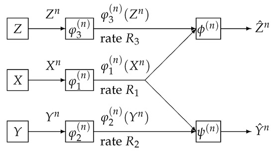
Figure 4. One helper source coding system investigated by Wyner.

A rate triple $(R_1,R_2,R_3)$ is $\epsilon$-achievable if, for any $\delta >0$, there exist a positive integer $n_0=n_0(\epsilon ,\delta )$ and a sequence of three encoders and two decoder functions $\{({\phi }_1^{(n)},{\phi }_2^{(n)},$${\phi }_3^{(n)},{\psi }^{(n)},$ ${\varphi }^{(n)}{)\}}_{n\ge n_0}$ such that, for $n\ge n_0(\epsilon ,\delta )$,

$$\begin{array}{c}\frac{1}{n}log\left|\right|{\phi }_i^{(n)}\left|\right|\le R_i+\delta fori=1,2,3,{\mathrm{P}}_{\mathrm{e}}^{(n)}({\phi }_1^{(n)},{\phi }_2^{(n)},{\phi }_3^{(n)},{\psi }^{(n)},{\varphi }^{(n)})\le \epsilon .\hfill \end{array}$$

The rate region ${\mathcal{R}}_{\mathrm{W}}(\epsilon |p_{XYZ})$ is defined by

$$\begin{array}{c}{\mathcal{R}}_{\mathrm{W}}(\epsilon |p_{XYZ}):=\{(R_1,R_2,R_3):(R_1,R_2,R_3)is\epsilon -\mathrm{achievable}\mathrm{for}{p}_{XYZ}\}.\hfill \end{array}$$

Furthermore, define

$${\mathcal{R}}_{\mathrm{W}}(p_{XYZ}):=\bigcap _{\epsilon \in (0,1)}{\mathcal{R}}_{\mathrm{W}}(\epsilon |p_{XYZ}).$$

We can show that the two rate regions ${\mathcal{R}}_{\mathrm{W}}(\epsilon |$$p_{XYZ})$, $\epsilon \in (0,1)$ and ${\mathcal{R}}_{\mathrm{W}}(p_{XYZ})$ satisfy the following property.

Property 5.

(a) 

The regions ${\mathcal{R}}_{\mathrm{W}}(\epsilon |p_{XYZ})$, $\epsilon \in (0,1)$, and ${\mathcal{R}}_{\mathrm{W}}($$p_{XYZ})$ are closed convex sets of ${\mathbb{R}}_{+}^3$.

(b) 

We set

$$\begin{array}{c}{\mathcal{R}}_{\mathrm{W}}(n,\epsilon |p_{XYZ})=\{(R_1,R_2,R_3):Thereexists({\phi }_1^{(n)},{\phi }_2^{(n)},{\phi }_3^{(n)},{\psi }^{(n)})suchthat\hfill \\ \frac{1}{n}log\left|\right|{\phi }_i^{(n)}\left|\right|\le R_i,i=1,2,3,{\mathrm{P}}_{\mathrm{e}}^{(n)}({\phi }_1^{(n)},{\phi }_2^{(n)},{\phi }_3^{(n)},{\psi }^{(n)})\le \epsilon \},\hfill \end{array}$$

which is called the $(n,\epsilon )$-rate region. Using ${\mathcal{R}}_{\mathrm{W}}(n,$$\epsilon |p_{XYZ})$, ${\mathcal{R}}_{\mathrm{W}}(\epsilon |p_{XYZ})$ can be expressed as

$$\begin{array}{cc}\hfill {\mathcal{R}}_{\mathrm{W}}(\epsilon |p_{XYZ})& =\mathrm{cl}\left(\bigcup _{m\ge 1}\bigcap _{n\ge m}{\mathcal{R}}_{\mathrm{W}}(n,\epsilon |p_{XYZ})\right).\hfill \end{array}$$

It is well known that ${\mathcal{R}}_{\mathrm{W}}(p_{XYZ})$ was determined by Wyner. To describe his result, we introduce an auxiliary random variable U taking values in a finite set $\mathcal{U}$. We assume that the joint distribution of $(U,X,Y,Z)$ is

$$p_{UXY}(u,x,y,z)=p_U(u)p_{X|U}(x|u)p_{YZ|X}(y,z|x).$$

The above condition is equivalent to $U\leftrightarrow X\leftrightarrow YZ$. Define the set of probability distribution on $\mathcal{U}$ $\times \mathcal{X}$ $\times \mathcal{Y}$ $\times \mathcal{Z}$ by

$$\begin{array}{cc}\hfill \mathcal{P}(p_{XYZ}):=& \{p=p_{UXYZ}:|\mathcal{U}|\le |\mathcal{X}|+2,U\leftrightarrow X\leftrightarrow YZ\}.\hfill \end{array}$$

Set

$$\begin{array}{cc}\hfill \mathcal{R}(p)& :=\begin{array}{c}\{(R_1,R_2,R_3):R_1,R_2,R_3\ge 0,\hfill \\ \begin{array}{ccc}\hfill R_1& \ge & I_p(X;U),R_2\ge H_p(Y|U),R_3\ge H_p(Z|U)\},\hfill \end{array}\hfill \end{array}\hfill \\ \hfill \mathcal{R}(p_{XYZ})& :=\bigcup _{p\in \mathcal{P}(p_{XYZ})}\mathcal{R}(p).\hfill \end{array}$$

We can show that the region $\mathcal{R}(p_{XYZ})$ satisfies the following property.

Property 6.

(a) 

The region $\mathcal{R}(p_{XYZ})$ is a closed convex subset of ${\mathbb{R}}_{+}^3$.

(b) 

For any $p_{XYZ}$, and any $\gamma \in [0,1]$, we have

$$\begin{array}{c}\underset{(R_1,R_2,R_3)\in \mathcal{R}(p_{XY})}{min}(R_1+\overline{\gamma }{R}_2+\gamma R_3)=\overline{\gamma }{H}_p(Y)+\gamma H_p(Z).\hfill \end{array}$$

(41)

The minimun is attained by $(R_1,R_2,R_3)=(0,H_p(Y),$$H_p(Z))$. This result implies that

$$\begin{array}{c}\mathcal{R}(p_{XYZ})\subseteq \begin{array}{c}{\displaystyle \left[\bigcap _{\gamma \in [0,1]}\{(R_1,R_2,R_3):R_1+\overline{\gamma }{R}_2+\gamma R_3\ge \overline{\gamma }{H}_p(Y)+\gamma H_p(Z)\}\right]\cap {\mathbb{R}}_{+}^3.}\hfill \end{array}\hfill \end{array}$$

Furthermore, the point $(0,H_p(Y),H_p(Z))$ always belongs to $\mathcal{R}(p_{XYZ})$.

The rate region ${\mathcal{R}}_{\mathrm{W}}(p_{XYZ})$ was determined by Wyner [2]. His result is the following.

Theorem 4

(Wyner [2]).

$$\begin{array}{c}{\mathcal{R}}_{\mathrm{W}}(p_{XYZ})=\mathcal{R}(p_{XYZ}).\hfill \end{array}$$

On the strong converse theorem, Csiszár and Körner [21] obtained the following.

Theorem 5

(Csiszár and Körner [21]). For each fixed ε$\in (0,1)$, we have

$$\begin{array}{c}\hfill {\mathcal{R}}_{\mathrm{W}}(\epsilon |p_{XYZ})=\mathcal{R}(p_{XYZ}).\end{array}$$

To examine a rate of convergence for the error probability of decoding to tend to one as $n\to \infty$ for $(R_1,R_2,R_3)$ $\notin {\mathcal{R}}_{\mathrm{W}}(p_{XYZ})$, we define the following quantity. Set

$$\begin{array}{c}{\mathrm{P}}_{\mathrm{c}}^{(n)}({\phi }_1^{(n)},{\phi }_2^{(n)},{\phi }_3^{(n)},{\psi }^{(n)},{\varphi }^{(n)}):=1-{\mathrm{P}}_{\mathrm{e}}^{(n)}({\phi }_1^{(n)},{\phi }_2^{(n)},{\phi }_3^{(n)},{\psi }^{(n)},{\varphi }^{(n)}),\hfill \\ G^{(n)}(R_1,R_2,R_3|p_{XYZ}):=\underset{\genfrac{}{}{0pt}{}{({\phi }_1^{(n)},{\phi }_2^{(n)},{\phi }_3^{(n)},}{\genfrac{}{}{0pt}{}{{\psi }^{(n)},{\varphi }^{(n)}):}{\genfrac{}{}{0pt}{}{(1/n)log\parallel {\phi }_i^{(n)}\parallel }{\le R_i,i=1,2,3}}}}{min}\left(-\frac{1}{n}\right)log{\mathrm{P}}_{\mathrm{c}}^{(n)}({\phi }_1^{(n)},{\phi }_2^{(n)},{\phi }_3^{(n)},{\psi }^{(n)},{\varphi }^{(n)}),\hfill \\ G(R_1,R_2,R_3|p_{XYZ}):=\underset{n\to \infty }{lim}{G}^{(n)}(R_1,R_2,R_3|p_{XYZ}),\hfill \\ \mathcal{G}(p_{XYZ}):=\{(R_1,R_2,R_3,G):G\ge G(R_1,R_2,R_3|p_{XYZ})\}.\hfill \end{array}$$

By time sharing, we have that

$$\begin{array}{c}{G}^{(n+m)}\left(\left.\frac{n{R}_1+m{R}_1^{\prime }}{n+m},\frac{n{R}_2+m{R}_2^{\prime }}{n+m},\frac{n{R}_2+m{R}_2^{\prime }}{n+m}\right|p_{XYZ}\right)\hfill \\ \le \frac{n{G}^{(n)}(R_1,R_2,R_3|p_{XYZ})+m{G}^{(m)}(R_1^{\prime },R_2^{\prime },R_3^{\prime }|p_{XYZ})}{n+m}.\hfill \end{array}$$

(42)

Choosing $R=R^{\prime }$ in (42), we obtain the following subadditivity property on $\{G^{(n)}(R_1,R_2,R_3|p_{XYZ})$ ${\}}_{n\ge 1}$:

$$\begin{array}{c}{G}^{(n+m)}(R_1,R_2,R_3|p_{XYZ})\le \frac{n{G}^{(n)}(R_1,R_2,R_3|p_{XYZ})+m{G}^{(m)}(R_1,R_2,R_3|p_{XYZ})}{n+m},\hfill \end{array}$$

from which we have that $G(R_1,R_2,R_3|p_{XYZ})$ exists and satisfies the following:

$$\begin{array}{c}G(R_1,R_2,R_3|p_{XYZ})=\underset{n\ge 1}{inf}{G}^{(n)}(R_1,R_2,R_3|p_{XYZ}).\hfill \end{array}$$

The exponent function $G(R_1,R_2,R_3|p_{XYZ})$ is a convex function of $(R_1,R_2,R_3)$. In fact, by time sharing, we have that

$$\begin{array}{c}{G}^{(n+m)}\left(\left.\frac{n{R}_1+m{R}_1^{\prime }}{n+m},\frac{n{R}_2+m{R}_2^{\prime }}{n+m},\frac{n{R}_2+m{R}_2^{\prime }}{n+m}\right|p_{XYZ}\right)\hfill \\ \le \frac{n{G}^{(n)}(R_1,R_2,R_3|p_{XYZ})+m{G}^{(m)}(R_1^{\prime },R_2^{\prime },R_3^{\prime }|p_{XYZ})}{n+m},\hfill \end{array}$$

from which we have that for any $\alpha \in [0,1]$

$$\begin{array}{c}G(\alpha R_1+\overline{\alpha }{R}_1^{\prime },\alpha R_2+\overline{\alpha }{R}_2^{\prime },\alpha R_3+\overline{\alpha }{R}_3^{\prime }|p_{XYZ})\le \alpha G(R_1,R_2,R_3|p_{XYZ})+\overline{\alpha }G(R_1^{\prime },R_2^{\prime },R_3^{\prime }|p_{XYZ}).\hfill \end{array}$$

The region $\mathcal{G}(p_{XYZ})$ is also a closed convex set. Our main aim is to find an explicit characterization of $\mathcal{G}(p_{XYZ})$. In this paper, we derive an explicit outer bound of $\mathcal{G}$ $(p_{XYZ})$ whose section by the plane $G=0$ coincides with ${\mathcal{R}}_{\mathrm{W}}(p_{XYZ})$. We first explain that the region $\mathcal{R}(p_{XYZ})$ has another expression using the supporting hyperplane. We define two sets of probability distributions on $\mathcal{U}$ $\times \mathcal{X}$ $\times \mathcal{Y}$ $\times \mathcal{Z}$ by

$$\begin{array}{c}{\mathcal{P}}_{\mathrm{sh}}(p_{XYZ}):=\{p=p_{UXYZ}:\left|\mathcal{U}\right|\le \left|\mathcal{X}\right|,U\leftrightarrow X\leftrightarrow YZ\},\hfill \\ \mathcal{Q}(p_{YZ|X}):=\{q=q_{UXYZ}:\left|\mathcal{U}\right|\le \left|\mathcal{X}\right|,p_{YZ|X}=q_{YZ|X},U\leftrightarrow X\leftrightarrow YZ\}.\hfill \end{array}$$

For $(\mu ,\gamma )\in {[0,1]}^2$, set

$$\begin{array}{c}{R}^{(\mu ,\gamma )}(p_{XYZ}):=\underset{p\in {\mathcal{P}}_{\mathrm{sh}}(p_{XYZ})}{max}\left\{\mu I_p(X;U)+\overline{\mu }(\overline{\gamma }{H}_p(Y|U)+\gamma H_p(Z|U))\right\}.\hfill \end{array}$$

Furthermore, define

$$\begin{array}{c}{\mathcal{R}}_{\mathrm{sh}}(p_{XYZ})=\bigcap _{(\mu ,\gamma )\in {[0,1]}^2}\{(R_1,R_2,R_3):\mu R_1+\overline{\mu }(\overline{\gamma }{R}_2+\gamma R_3)\ge R^{(\mu ,\gamma )}(p_{XYZ})\}.\hfill \end{array}$$

Then, we have the following property.

Property 7.

(a) 

The bound $\left|\mathcal{U}\right|\le \left|\mathcal{X}\right|$ is sufficient to describe $R^{(\mu )}($$p_{XYZ})$.

(b) 

For every $(\mu ,\gamma )\in {[0,1]}^2$, we have

$$\begin{array}{c}\underset{(R_1,R_2,R_3)\in \mathcal{R}(p_{XYZ})}{min}\{\mu R_1+\overline{\mu }(\overline{\gamma }{R}_2+\gamma R_3)\}=R^{(\mu ,\gamma )}(p_{XYZ}).\hfill \end{array}$$

(c) 

For any $p_{XYZ},$ we have

$${\mathcal{R}}_{\mathrm{sh}}(p_{XYZ})=\mathcal{R}(p_{XYZ}).$$

(43)

For $(\mu ,\gamma ,\alpha )\in {[0,1]}^3$, and for $q=q_{UXYZ}\in \mathcal{Q}(p_{YZ|X})$, define

$$\begin{array}{c}{\omega }_{q|p_X}^{(\mu ,\gamma ,\alpha )}(x,y,z|u):=\overline{\alpha }log\frac{q_X(x)}{p_X(x)}+\alpha \left[\mu log\frac{q_{X|U}(x|u)}{p_X(x)}+\overline{\mu }\left(\overline{\gamma }log\frac{1}{q_{Y|U}(y|u)}+\gamma log\frac{1}{q_{Z|U}(z|u)}\right)\right],\hfill \\ f_{q|p_X}^{(\mu ,\gamma ,\alpha )}(x,y,z|u):=exp\left\{-{\omega }_{q|p_X}^{(\mu ,\gamma ,\alpha )}(x,y,z|u)\right\},\hfill \\ {\Omega }^{(\mu ,\gamma ,\alpha )}(q|p_X):=-log{\mathrm{E}}_q\left[f_{q|p_X}^{(\mu ,\gamma ,\alpha )}(X,Y,Z|U)\right],{\Omega }^{(\mu ,\gamma ,\alpha )}(p_{XYZ}):=\underset{\genfrac{}{}{0pt}{}{}{q\in \mathcal{Q}(p_{YZ|X})}}{min}{\Omega }^{(\mu ,\gamma ,\alpha )}(q|p_X),\hfill \\ F^{(\mu ,\gamma ,\alpha )}(\mu R_1+\overline{\gamma }{R}_2+\gamma R_3):=\frac{{\Omega }^{(\mu ,\gamma ,\alpha )}(p_{XYZ})-\alpha [\mu R_1+\overline{\mu }(\overline{\gamma }{R}_2+\gamma R_3)]}{2+\alpha \overline{\mu }},\hfill \\ F(R_1,R_2,R_3|p_{XYZ}):=\underset{(\mu ,\gamma ,\alpha )\in {[0,1]}^3,}{sup}{F}^{(\mu ,\gamma ,\alpha )}(\mu R_1+\overline{\mu }(\overline{\gamma }{R}_2+\gamma R_3)|p_{XYZ}).\hfill \end{array}$$

We next define a function serving as a lower bound of $F(R_1,R_2,R_3|p_{XYZ})$. For each $p=p_{UXYZ}\in {\mathcal{P}}_{\mathrm{sh}}(p_{XYZ})$, define

$$\begin{array}{c}{\tilde{\omega }}_p^{(\mu ,\gamma )}(x,y,z|u):=\mu log\frac{p_{X|U}(x|u)}{p_X(x)}+\overline{\mu }\left(\overline{\gamma }log\frac{1}{p_{Y|U}(y|u)}+\gamma log\frac{1}{p_{Z|U}(z|u)}\right),\hfill \\ {\tilde{\Omega }}^{(\mu ,\gamma ,\lambda )}(p):=-log{\mathrm{E}}_p\left[exp\left\{-\lambda {\omega }_p^{(\mu ,\gamma )}(X,Y,Z|U)\right\}\right],{\tilde{\Omega }}^{(\mu ,\gamma ,\lambda )}(p_{XYZ}):=\underset{\genfrac{}{}{0pt}{}{}{p\in {\mathcal{P}}_{\mathrm{sh}}(p_{XYZ})}}{min}{\tilde{\Omega }}^{(\mu ,\gamma ,\lambda )}(p).\hfill \end{array}$$

Furthermore, set

$$\begin{array}{c}{\underline{F}}^{(\mu ,\gamma ,\lambda )}(\mu R_1+\overline{\gamma }{R}_2+\gamma R_3|p_{XYZ}):=\frac{{\tilde{\Omega }}^{(\mu ,\gamma ,\lambda )}(p_{XYZ})-\lambda [\mu R_1+\overline{\mu }(\overline{\gamma }{R}_2+\gamma R_3)]}{2+\lambda (5-\mu )},\hfill \\ \underline{F}(R_1,R_2,R_3|p_{XYZ}):=\underset{\genfrac{}{}{0pt}{}{(\mu ,\gamma )\in {[0,1]}^2,}{\lambda \ge 0}}{sup}{\underline{F}}^{(\mu ,\gamma ,\lambda )}(\mu R_1+\overline{\mu }\overline{\gamma }{R}_2+\gamma R_3|p_{XYZ}).\hfill \end{array}$$

We can show that the above functions and sets satisfy the following property.

Property 8.

(a) 

The cardinality bound $\left|\mathcal{U}\right|\le \left|\mathcal{X}\right|$ in $\mathcal{Q}(p_{Y|X})$ is sufficient to describe the quantity ${\Omega }^{(\mu ,\alpha )}(p_{XY})$. Furthermore, the cardinality bound $\left|\mathcal{U}\right|\le \left|\mathcal{X}\right|$ in $\mathcal{Q}(p_{YZ|X})$ is sufficient to describe the quantity ${\tilde{\Omega }}^{(\mu ,\gamma ,\lambda )}(p_{XYZ})$.

(b) 

For any $R_1,R_2,R_3\ge 0$, we have

$$\begin{array}{c}F(R_1,R_2,R_3|p_{XYZ})\ge \underline{F}(R_1,R_2,R_3|p_{XYZ}).\hfill \end{array}$$

(c) 

For any $p=p_{UXY}\in {\mathcal{P}}_{\mathrm{sh}}(p_{XY})$ and any $(\mu ,\gamma ,\lambda$$)\in [0,$${1]}^3$, we have

$$0\le {\tilde{\Omega }}^{(\mu ,\gamma ,\lambda )}(p)\le \mu log\left|\mathcal{X}\right|+\overline{\mu }{log(|\mathcal{Y}|}^{\overline{\gamma }}{\left|\mathcal{Z}\right|}^{\gamma }).$$

(44)

(d) 

Fix any $p=p_{UXYZ}\in {\mathcal{P}}_{\mathrm{sh}}(p_{XYZ})$ and $(\mu ,\gamma )\in {[0,1]}^2$. We define a probability distribution $p^{(\lambda )}=p_{UXYZ}^{(\lambda )}$ by

$$\begin{array}{c}{p}^{(\lambda )}(u,x,y,z):=\frac{p(u,x,y,z)exp\left\{-\lambda {\omega }_p^{(\mu ,\gamma )}(x,y,z|u)\right\}}{{\mathrm{E}}_p\left[exp\left\{-\lambda {\omega }_p^{(\mu ,\gamma )}(X,Y,Z|U)\right\}\right]}.\hfill \end{array}$$

Then, for $\lambda \in [0,1/2]$, ${\tilde{\Omega }}^{(\mu ,\gamma ,\lambda )}(p)$ is twice differentiable. Furthermore, for $\lambda \in [0,1/2]$, we have

$$\begin{array}{c}\frac{\mathrm{d}}{\mathrm{d}\lambda }{\tilde{\Omega }}^{(\mu ,\gamma ,\lambda )}(p)={\mathrm{E}}_{p^{(\lambda )}}\left[{\omega }_p^{(\mu ,\gamma )}(X,Y,Z|U)\right],\frac{{\mathrm{d}}^2}{\mathrm{d}{\lambda }^2}{\tilde{\Omega }}^{(\mu ,\gamma ,\lambda )}(p)=-{\mathrm{Var}}_{p^{(\lambda )}}\left[{\omega }_p^{(\mu ,\gamma )}(X,Y,Z|U)\right].\hfill \end{array}$$

The second equality implies that ${\tilde{\Omega }}^{(\mu ,\gamma ,\lambda )}(p)$ is a concave function of $\lambda \in [0,1/2]$.

(e) 

For $(\mu ,\gamma ,\lambda )\in {[0,1]}^2\times [0,1/2]$, define

$$\begin{array}{cc}\hfill {\rho }^{(\mu ,\gamma ,\lambda )}(p_{XYZ})& :=\underset{\genfrac{}{}{0pt}{}{(\nu ,p)\in [0,\lambda ]\times {\mathcal{P}}_{\mathrm{sh}}(p_{XYZ}):}{{\tilde{\Omega }}^{(\mu ,\gamma ,\lambda )}(p)={\tilde{\Omega }}^{(\mu ,\gamma ,\lambda )}(p_{XYZ})}}{max}{\mathrm{Var}}_{p^{(\nu )}}\left[{\tilde{\omega }}_p^{(\mu ,\gamma )}(X,Y,Z|U)\right],\hfill \end{array}$$

and set

$$\begin{array}{c}\rho =\rho (p_{XYZ}):=\underset{(\mu ,\gamma ,\lambda )\in {[0,1]}^2\times [0,1/2]}{max}{\rho }^{(\mu ,\gamma ,\lambda )}(p_{XYZ}).\hfill \end{array}$$

Then, we have $\rho (p_{XYZ})<\infty$. Furthermore, for any $(\mu ,\gamma ,\lambda )$ $\in {[0,1]}^2\times [0,1/2]$, we have

$${\tilde{\Omega }}^{(\mu ,\gamma ,\lambda )}(p_{XYZ})\ge \lambda R^{(\mu ,\gamma )}(p_{XYZ})-\frac{{\lambda }^2}{2}\rho (p_{XYZ}).$$

(f) 

For every $\tau \in (0,(1/2)\rho (p_{XYZ}))$, the condition $(R_1+\tau ,$$R_2+\tau ,R_3+\tau )\notin \mathcal{R}(p_{XYZ})$ implies

$$\begin{array}{c}F(R_1,R_2,R_3|p_{XYZ})>\frac{\rho (p_{XYZ})}{4}·g^2\left(\frac{\tau }{\rho (p_{XYZ})}\right)>0.\hfill \end{array}$$

Since proofs of the results stated in Property 8 are quite parallel with those of the results stated in Property 4, we omit them. Our main result is the following.

Theorem 6.

For any $R_1,R_2,$$R_3\ge 0$, any $p_{XYZ}$, and for any $({\phi }_1^{(n)},$${\phi }_2^{(n)},$${\phi }_3^{(n)},$ ${\psi }^{(n)},{\varphi }^{(n)})$ satisfying $(1/n)log\left|\right|{\phi }_i^{(n)}\left|\right|$$\le R_i,i=1,2,3,$ we have

$$\begin{array}{c}{\mathrm{P}}_{\mathrm{c}}^{(n)}({\phi }_1^{(n)},{\phi }_2^{(n)},{\phi }_3^{(n)},{\psi }^{(n)},{\varphi }^{(n)})\le 7exp\left\{-nF(R_1,R_2,R_3|p_{XYZ})\right\}.\hfill \end{array}$$

It follows from Theorem 6 and Property 8 part d) that, if $(R_1,R_2,R_3)$ is outside the capacity region, then the error probability of decoding goes to one exponentially and its exponent is not below $F(R_1,R_2,R_3|p_{XYZ})$. It immediately follows from Theorem 3 that we have the following corollary.

Corollary 4.

$$\begin{array}{c}G(R_1,R_2,R_3|p_{XYZ})\ge F(R_1,R_2,R_3|p_{XYZ}),\hfill \\ \mathcal{G}(p_{XYZ})\subseteq \overline{\mathcal{G}}(p_{XYZ})=\left\{(R_1,R_2,R_3,G):G\ge F(R_1,R_2,R_3|p_{XYZ})\right\}.\hfill \end{array}$$

Proof of Theorem 6 is quite parallel with that of Theorem 3. We omit the detail of the proof. From Theorem 6 and Property 8 part e, we can obtain an explicit outer bound of ${\mathcal{R}}_{\mathrm{W}}(\epsilon |p_{XYZ})$ with an asymptotically vanishing deviation from ${\mathcal{R}}_{\mathrm{W}}(p_{XYZ})$$=\mathcal{R}(p_{XYZ})$. The strong converse theorem established by Csiszár and Körner [21] immediately follows from this corollary. To describe this outer bound, for $\kappa >0$, we set

$$\begin{array}{c}\mathcal{R}(p_{XYZ})-\kappa (1,1,1):=\{(R_1-\kappa ,R_2-\kappa ,R_3-\kappa ):(R_1,R_2,R_3)\in \mathcal{R}(p_{XYZ})\},\hfill \end{array}$$

which serves as an outer bound of $\mathcal{R}(p_{XYZ})$. For each fixed $\epsilon \in (0,1)$, we define ${\tilde{\kappa }}_n$$={\tilde{\kappa }}_n(\epsilon ,\rho (p_{XYZ}))$ by

$$\begin{array}{ccc}\hfill {\tilde{\kappa }}_n& :=& \rho (p_{XY})\vartheta \left(\sqrt{\frac{4}{n\rho (p_{XY})}log\left(\frac{7}{1-\epsilon }\right)}\right)\hfill \\ & \stackrel{(\mathrm{a})}{=}& 2\sqrt{\frac{\rho (p_{XY})}{n}log\left(\frac{7}{1-\epsilon }\right)}+\frac{5}{n}log\left(\frac{7}{1-\epsilon }\right).\hfill \end{array}$$

(45)

Step (a) follows from $\vartheta (a)=a+(5/4)a^2$. Since ${\tilde{\kappa }}_n\to 0$ as $n\to \infty$, we have the smallest positive integer $n_1=n_1(\epsilon ,\rho (p_{XYZ}))$ such that ${\tilde{\kappa }}_n\le (1/2)\rho (p_{XYZ})$ for $n\ge n_1$. From Theorem 6 and Property 8 part e, we have the following corollary.

Corollary 5.

For each fixed $\epsilon \in (0,1)$, we choose the above positive integer $n_1=$$n_1(\epsilon ,\rho (p_{XYZ}))$. Then, for any $n\ge n_1$, we have

$$\begin{array}{cc}\hfill {\mathcal{R}}_{\mathrm{W}}(\epsilon |p_{XYZ})& \subseteq \mathcal{R}(p_{XYZ})-{\tilde{\kappa }}_n(0,1,1).\hfill \end{array}$$

The above result together with

$$\begin{array}{cc}\hfill {\mathcal{R}}_{\mathrm{W}}(\epsilon |p_{XYZ})& =\mathrm{cl}\left(\bigcup _{m\ge 1}\bigcap _{n\ge m}{\mathcal{R}}_{\mathrm{W}}(n,\epsilon |p_{XYZ})\right)\hfill \end{array}$$

yields that for each fixed $\epsilon \in (0,1)$, we have

$$\begin{array}{c}{\mathcal{R}}_{\mathrm{W}}(\epsilon |p_{XYZ})={\mathcal{R}}_{\mathrm{W}}(p_{XYZ})=\mathcal{R}(p_{XYZ}).\hfill \end{array}$$

This recovers the strong converse theorem proved by Csiszár and Körner [21].

Proof of this corollary is quite parallel with that of Corollary 2. We omit the detail.

6. Conclusions

For the AWZ system, the one helper source coding system posed by Ahlswede, Körner [1] and Wyner [2], we have derived an explicit lower bound of the optimal exponent function $G(R_1,R_2|p_{XY})$ on the correct probability of decoding for $(R_1,R_2)\notin {\mathcal{R}}_{\mathrm{WZ}}(p_{XY})$. We have described this result in Theorem 3. Furthermore, for the source coding system posed and investigated Wyner [2], we have obtained an explicit lower bound of the optimal exponent function $G(R_1,R_2,R_3|p_{XYZ})$ on the correct probability of decoding for $(R_1,R_2,R_3)\notin {\mathcal{R}}_{\mathrm{W}}(p_{XYZ})$. We have described this result in Theorem 6. The determination problems of $G(R_1,R_2|p_{XY})$ and $G(R_1,R_2,R_3|p_{XYZ})$ still remain to be resolved. Those problems are our future works.

References

- Ahlswede, R.F.; Körner, J. Source coding with side information and a converse for degraded broadcast channels. IEEE Trans. Inf. Theory 1975, 21, 629–637. [Google Scholar] [CrossRef]
- Wyner, A.D. On source coding with side information at the decoder. IEEE Trans. Inf. Theory 1975, 21, 294–300. [Google Scholar] [CrossRef]
- Csiszár, I.; Longo, G. On the exponent function for source coding and for testing simple statistical hypotheses. Studia Sci. Math. Hungar 1971, 6, 181–191. [Google Scholar]
- Slepian, D.; Wolf, J.K. Noiseless coding of correlated information sources. IEEE Trans. Inf. Theory 1973, 19, 471–480. [Google Scholar] [CrossRef]
- Oohama, Y.; Han, T.S. Universal coding for the Slepian-wolf data compression system and the strong converse theorem. IEEE Trans. Inf. Theory 1994, 40, 1908–1919. [Google Scholar] [CrossRef]
- Ahlswede, R.; Gács, P.; Körner, J. Bounds on conditional probabilities with applications in multi-user communication. Probab. Theory Relat. Fields 1976, 34, 157–177. [Google Scholar] [CrossRef]
- Gu, W.; Effors, M. A strong converse for a collection of network source coding problems. In Proceedings of the IEEE International Symposium on Information Theory, Soul, Korea, 28 June–3 July 2009; pp. 2316–2320. [Google Scholar]
- Oohama, Y. Strong converse exponent for degraded broadcast channels at rates outside the capacity region. In Proceedings of the 2015 IEEE International Symposium on Information Theory, Hong Kong, China, 14–19 June 2015; pp. 939–943. [Google Scholar]
- Oohama, Y. Strong converse theorems for degraded broadcast channels with feedback. In Proceedings of the 2015 IEEE International Symposium on Information Theory, Hong Kong, China, 14–19 June 2015; pp. 2510–2514. [Google Scholar]
- Oohama, Y. Exponent function for asymmetric broadcast channels at rates outside the capacity region. In Proceedings of the 2016 IEEE International Symposium on Information Theory and its Applications, Monterey, CA, USA, 30 October–2 Novomber 2016; pp. 568–572. [Google Scholar]
- Oohama, Y. New Strong Converse for Asymmetric Broadcast Channels. Available online: https://arxiv.org/pdf/1604.02901.pdf (accessed on 31 May 2019).
- Oohama, Y. Exponential strong converse for source coding with side information at the decoder. Entropy 2018, 20, 352. [Google Scholar] [CrossRef]
- Watanabe, S. A converse bound on Wyner-Ahlswede-Körner network via Gray–Wyner network. In Proceedings of the 2017 IEEE Information Theory Workshop (ITW), Kaohsiung, Taiwan, 6–10 November 2017; pp. 81–85. [Google Scholar]
- Liu, J.; van Handel, R.; Verdu, S. Beyond the blowing-up lemma: Sharp converses via reverse hypercontractivity. In Proceedings of the 2017 IEEE International Symposium on Information Theory (ISIT), Aachen, Germany, 25–30 June 2017; pp. 943–947. [Google Scholar]
- Watanabe, S. Second-order region for Gray–Wyner network. IEEE Trans. Inform. Theory 2017, 63, 1006–1018. [Google Scholar] [CrossRef]
- Liu, J. Dispersion bound for the Wyner-Ahlswede-Körner network via reverse hypercontractivity on types. In Proceedings of the 2018 IEEE International Symposium on Information Theory (ISIT), Vail, CO, USA, 17–22 June 2018; pp. 1854–1858. [Google Scholar]
- Watanabe, S.; Oohama, Y. Privacy amplification theorem for bounded storage eavesdropper. In Proceedings of the 2012 IEEE Information Theory Workshop (ITW), Lausanne, Switzerland, 3–7 September 2012; pp. 177–181. [Google Scholar]
- Oohama, Y.; Santoso, B. Information Theoretic Security for Side-Channel Attacks to the Shannon Cipher System. Available online: https://arxiv.org/pdf/1801.02563v5.pdf. (accessed on 31 May 2019).
- Santoso, B.; Oohama, Y. Information Theoretic Security for Shannon Cipher System under Side-Channel Attacks. Entropy 2019, 21, 469. [Google Scholar] [CrossRef]
- Oohama, Y. Exponent Function for One Helper Source Coding Problem at Rates outside the Rate Region. arXiv 2015, arXiv:1504.05891. [Google Scholar]
- Csiszár, I.; Körner, J. Information Theory: Coding Theorems for Discrete Memoryless Systems; Cambridge University Press: London, UK, 1981. [Google Scholar]
- Han, T.S. Information-Spectrum Methods in Information Theory; Springer Nature Switzerland AG: Basel, Switzerland, 2002. [Google Scholar]
© 2019 by the author. Licensee MDPI, Basel, Switzerland. This article is an open access article distributed under the terms and conditions of the Creative Commons Attribution (CC BY) license (http://creativecommons.org/licenses/by/4.0/).