Analytical Solutions of Fractional-Order Diffusion Equations by Natural Transform Decomposition Method


Abstract
1. Introduction
- (1)
- Two-dimensional fractional-order diffusion equation of the form:subject to the initial condition
- (2)
- Three-dimensional fractional-order diffusion equation is given bysubject to the initial condition
2. Preliminaries
3. Idea of Fractional Natural Transform Decomposition Method
4. Results
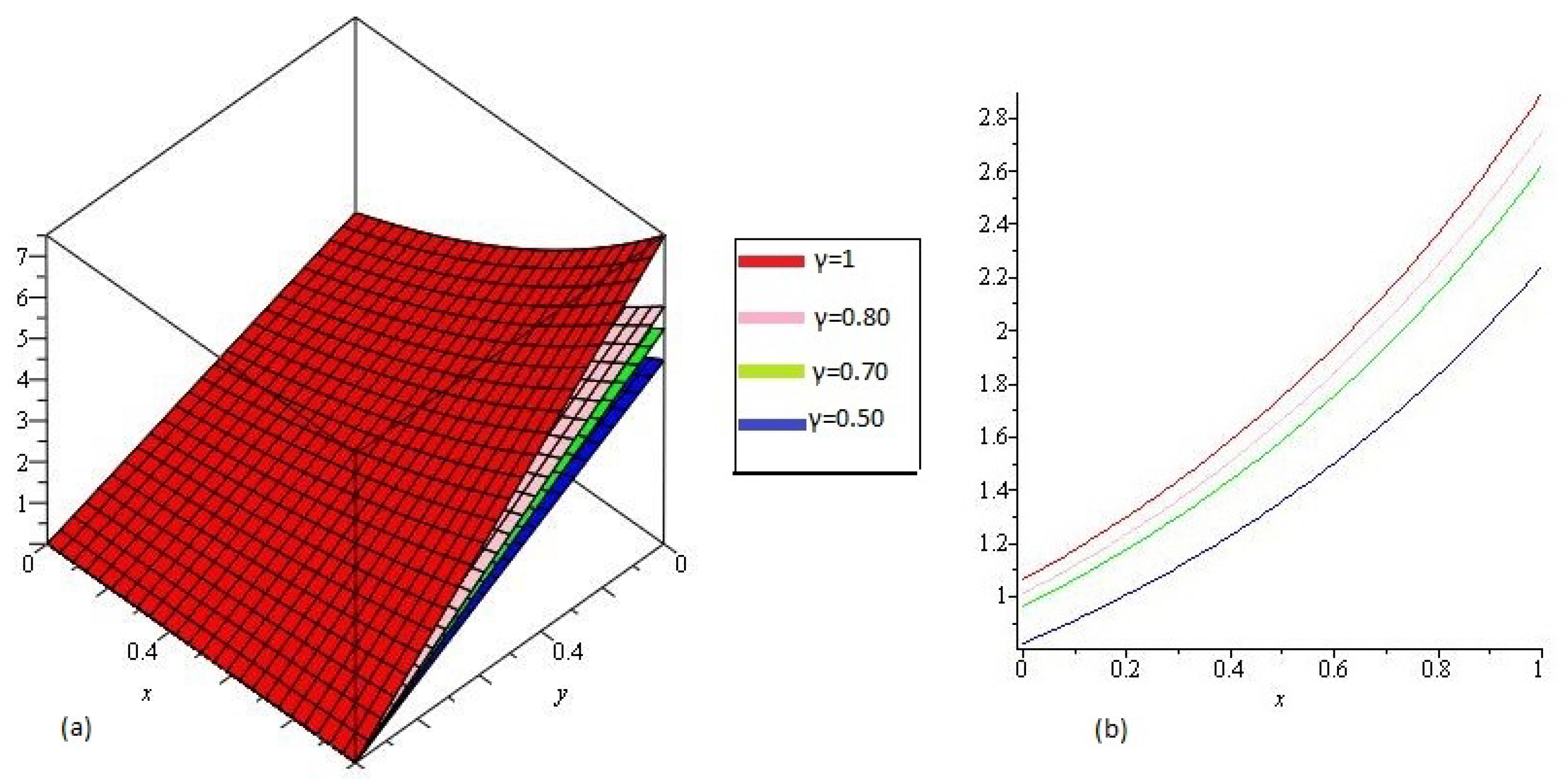
4.1. Example
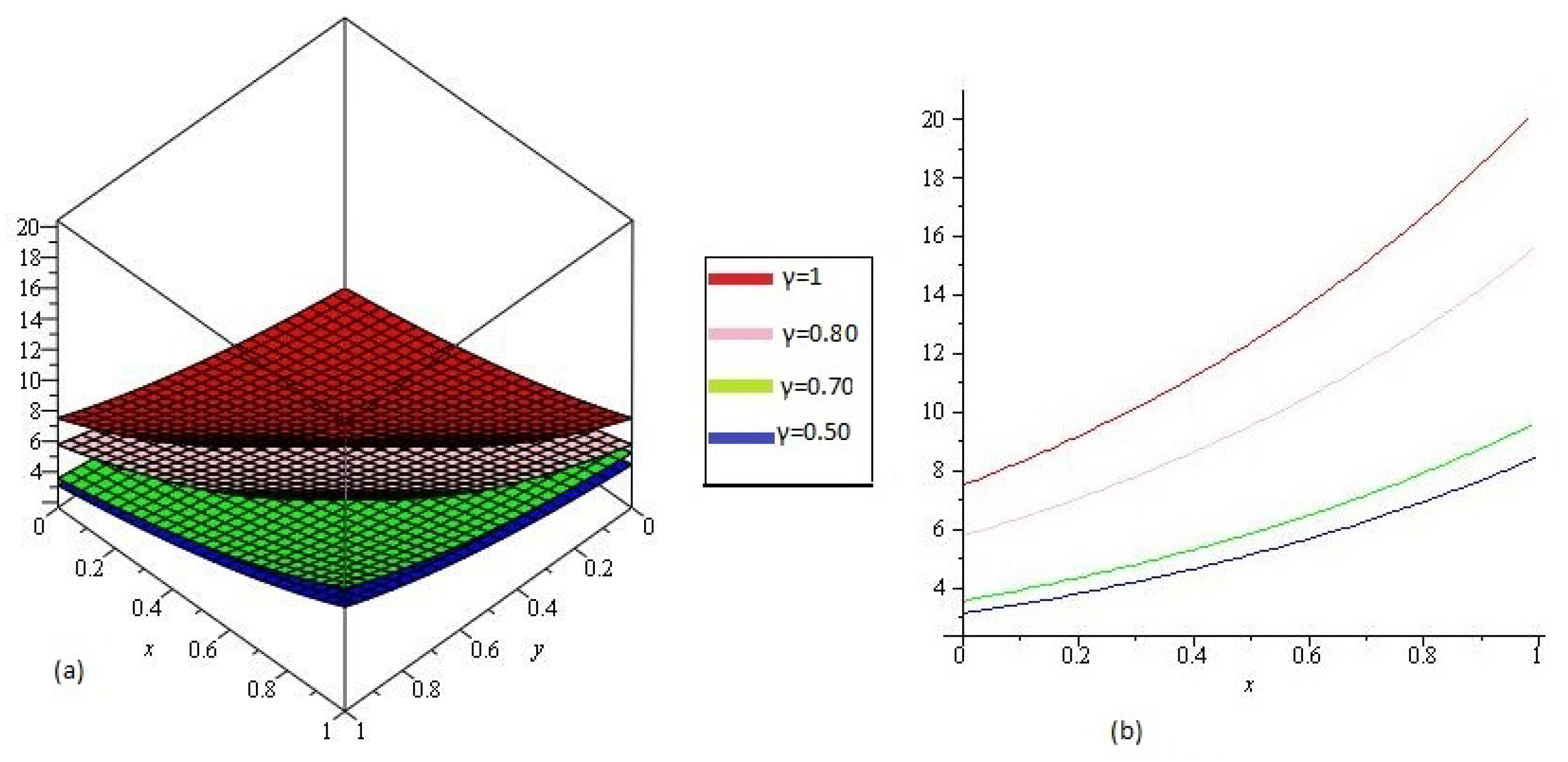
4.2. Example
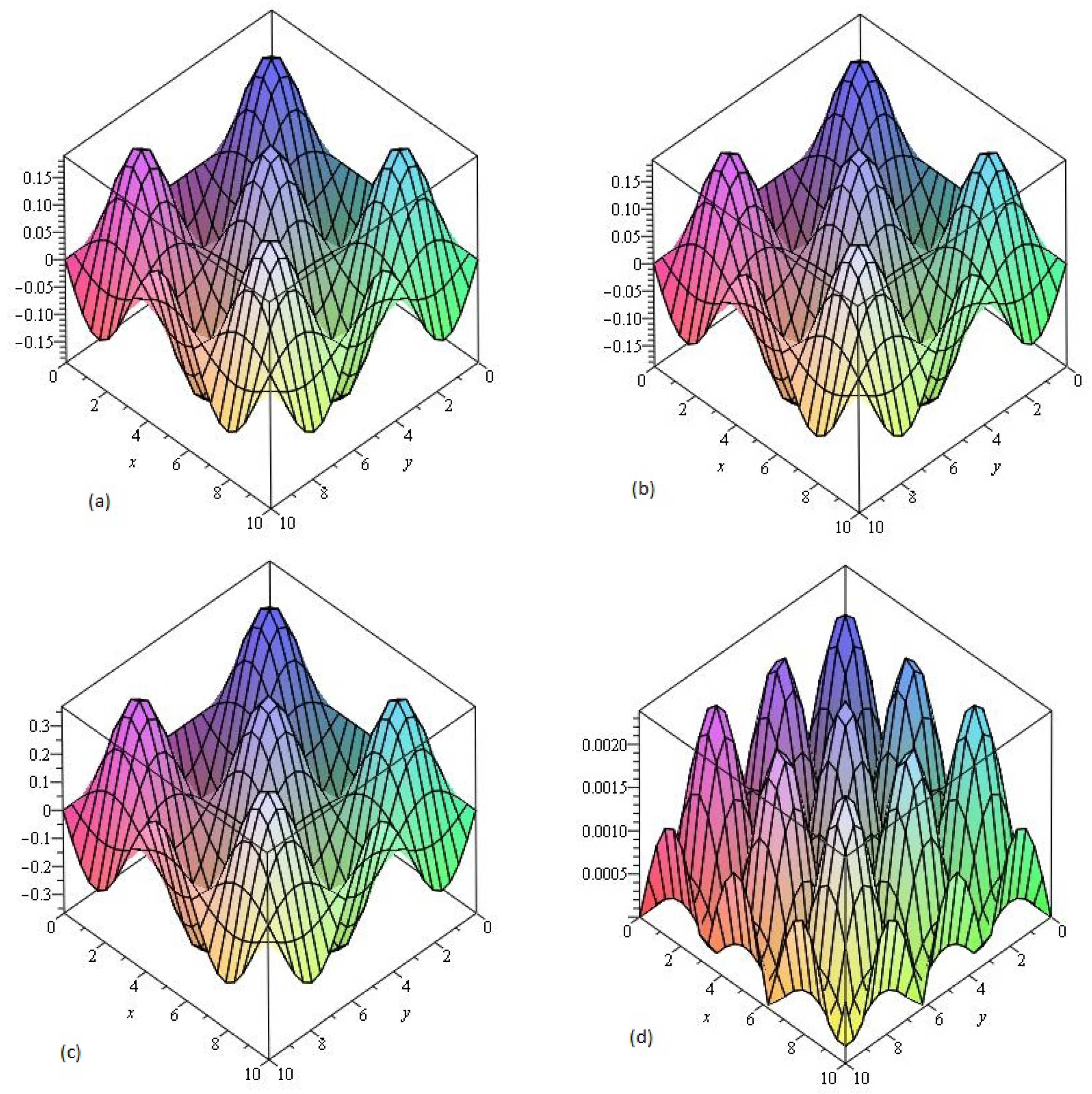
4.3. Example
5. Conclusions
Author Contributions
Funding
Acknowledgments
Conflicts of Interest
References
- Gómez-Aguilar, J.F.; Atangana, A. Fractional Hunter-Saxton equation involving partial operators with bi-order in Riemann-Liouville and Liouville-Caputo sense. Eur. Phys. J. Plus 2017, 132, 100. [Google Scholar] [CrossRef]
- Arshad, S.; Baleanu, D.; Huang, J.; Al Qurashi, M.; Tang, Y.; Zhao, Y. Finite Difference Method for Time-Space Fractional Advection–Diffusion Equations with Riesz Derivative. Entropy 2018, 20, 321. [Google Scholar] [CrossRef]
- Machado, J.A.T. Entropy analysis of integer and fractional dynamical systems. Nonlinear Dyn. 2010, 62, 371–378. [Google Scholar]
- Hoffmann, K.H.; Essex, C.; Schulzky, C. Fractional diffusion and entropy production. J. Non-Equilib. Thermodyn. 1998, 23, 166–175. [Google Scholar] [CrossRef]
- Magin, R.L.; Ingo, C. Entropy and information in a fractional order model of anomalous diffusion. IFAC Proc. 2012, 45, 428–433. [Google Scholar] [CrossRef]
- Ubriaco, M.R. Entropies based on fractional calculus. Phys. Lett. 2009, 373, 2516–2519. [Google Scholar] [CrossRef]
- Yépez-Martínez, H.; Gómez-Aguilar, F.; Sosa, I.O.; Reyes, J.M.; Torres-Jiménez, J. The Feng’s first integral method applied to the nonlinear mKdV space-time fractional partial differential equation. Rev. Mex. Fís. 2016, 62, 310–316. [Google Scholar]
- Ball, J.M.; Chen, G.Q.G. Entropy and convexity for nonlinear partial differential equations. Philos. Trans. R. Soc. Math. Phys. Eng. Sci. 2013, 371. [Google Scholar] [CrossRef]
- Shah, R.; Khan, H.; Arif, M.; Kumam, P. Application of Laplace-Adomian Decomposition Method for the Analytical Solution of Third-Order Dispersive Fractional Partial Differential Equations. Entropy 2019, 21, 335. [Google Scholar] [CrossRef]
- Sibatov, R.; Shulezhko, V.; Svetukhin, V. Fractional Derivative Phenomenology of Percolative Phonon-Assisted Hopping in Two-Dimensional Disordered Systems. Entropy 2017, 19, 463. [Google Scholar] [CrossRef]
- Jiang, J.; Feng, Y.; Li, S. Exact Solutions to the Fractional Differential Equations with Mixed Partial Derivatives. Axioms 2018, 7, 10. [Google Scholar] [CrossRef]
- Prehl, J.; Essex, C.; Hoffmann, K.H. Tsallis relative entropy and anomalous diffusion. Entropy 2012, 14, 701–716. [Google Scholar] [CrossRef]
- Cuahutenango-Barro, B.; Taneco-Hernández, M.A.; Gómez-Aguilar, J.F. On the solutions of fractional-time wave equation with memory effect involving operators with regular kernel. Chaos Solitons Fractals 2018, 115, 283–299. [Google Scholar] [CrossRef]
- Gómez-Gardeñes, J.; Latora, V. Entropy rate of diffusion processes on complex networks. Phys. Rev. 2008, 78, 065102. [Google Scholar] [CrossRef] [PubMed]
- Lopes, A.M.; Tenreiro Machado, J.A. Entropy Analysis of Soccer Dynamics. Entropy 2019, 21, 187. [Google Scholar] [CrossRef]
- Bejan, A. Second-law analysis in heat transfer and thermal design. Adv. Heat Transf. 1982, 15, 1–58. [Google Scholar]
- Bejan, A. A study of entropy generation in fundamental convective heat transfer. J. Heat Transf. 1979, 101, 718–725. [Google Scholar] [CrossRef]
- Syam, M.; Al-Refai, M. Solving fractional diffusion equation via the collocation method based on fractional legendre functions. Comput. Methods Phys. 2014, 2014, 381074. [Google Scholar] [CrossRef]
- Lenzi, E.; dos Santos, M.; Michels, F.; Mendes, R.; Evangelista, L. Solutions of some nonlinear diffusion equations and generalized entropy framework. Entropy 2013, 15, 3931–3940. [Google Scholar] [CrossRef]
- Prehl, J.; Boldt, F.; Hoffmann, K.; Essex, C. Symmetric fractional diffusion and entropy production. Entropy 2016, 18, 275. [Google Scholar] [CrossRef]
- Dehghan, M.; Abbaszadeh, M. A finite difference/finite element technique with error estimate for space fractional tempered diffusion-wave equation. Comput. Math. Appl. 2018, 75, 2903–2914. [Google Scholar] [CrossRef]
- Lei, S.L.; Huang, Y.C. Fast algorithms for high-order numerical methods for space-fractional diffusion equations. Int. J. Comput. Math. 2017, 94, 1062–1078. [Google Scholar] [CrossRef]
- Sepahvandzadeh, A.; Ghazanfari, B.; Asadian, N. Numerical Solution of Stochastic Generalized Fractional Diffusion Equation by Finite Difference Method. Math. Comput. Appl. 2018, 23, 53. [Google Scholar] [CrossRef]
- Tripathi, N.; Das, S.; Ong, S.; Jafari, H.; Al Qurashi, M. Solution of higher order nonlinear time-fractional reaction diffusion equation. Entropy 2016, 18, 329. [Google Scholar] [CrossRef]
- Shah, K.; Khalil, H.; Khan, R.A. Analytical solutions of fractional order diffusion equations by natural transform method. Iran. J. Sci. Technol. Trans. Sci. 2016, 92, 1479–1490. [Google Scholar] [CrossRef]
- Kumar, D.; Singh, J.; Kumar, S. Numerical computation of fractional multi-dimensional diffusion equations by using a modified homotopy perturbation method. J. Assoc. Arab. Univ. Basic Appl. Sci. 2015, 17, 20–26. [Google Scholar] [CrossRef]
- Zafarghandi, F.S.; Mohammadi, M.; Babolian, E.; Javadi, S. Radial basis functions method for solving the fractional diffusion equations. Appl. Math. Comput. 2019, 342, 224–246. [Google Scholar] [CrossRef]
- Luchko, Y. Entropy production rate of a one-dimensional alpha-fractional diffusion process. Axioms 2016, 5, 6. [Google Scholar] [CrossRef]
- Wei, S.; Chen, W.; Zhang, Y.; Wei, H.; Garrard, R.M. A local radial basis function collocation method to solve the variable-order time fractional diffusion equation in a two-dimensional irregular domain. Numer. Methods Partial. Differ. Equ. 2018, 34, 1209–1223. [Google Scholar] [CrossRef]
- Das, S. Analytical solution of a fractional diffusion equation by variational iteration method. Comput. Math. Appl. 2009, 57, 483–487. [Google Scholar] [CrossRef]
- Rawashdeh, M.S.; Maitama, S. Solving coupled system of nonlinear PDE’s using the natural decomposition method. Int. J. Pure Appl. Math. 2014, 92, 757–776. [Google Scholar] [CrossRef]
- Rawashdeh, M.S.; Maitama, S. Solving nonlinear ordinary differential equations using the NDM. J. Appl. Anal. Comput. 2015, 5, 77–88. [Google Scholar]
- Rawashdeh, M.; Maitama, S. Finding exact solutions of nonlinear PDEs using the natural decomposition method. Math. Methods Appl. Sci. 2017, 40, 223–236. [Google Scholar] [CrossRef]
- Cherif, M.H.; Ziane, D.; Belghaba, K. Fractional natural decomposition method for solving fractional system of nonlinear equations of unsteady flow of a polytropic gas. Nonlinear Stud. 2018, 25, 753–764. [Google Scholar]
- Eltayeb, H.; Abdalla, Y.T.; Bachar, I.; Khabir, M.H. Fractional Telegraph Equation and Its Solution by Natural Transform Decomposition Method. Symmetry 2019, 11, 334. [Google Scholar] [CrossRef]
- Abdel-Rady, A.S.; Rida, S.Z.; Arafa, A.A.M.; Abedl-Rahim, H.R. Natural transform for solving fractional models. J. Appl. Math. Phys. 2015, 3, 1633. [Google Scholar] [CrossRef]
- Belgacem, F.B.M.; Silambarasan, R. November. Advances in the natural transform. AIP Conf. Proc. 2012, 1493, 106–110. [Google Scholar]
- Khan, Z.H.; Khan, W.A. N-transform properties and applications. NUST J. Eng. Sci. 2008, 1, 127–133. [Google Scholar]
- Hilfer, R. Applications of Fractional Calculus in Physics; World Science Publishing: River Edge, NJ, USA, 2000. [Google Scholar]
- Podlubny, I. Fractional Differential Equations: An Introduction to Fractional Derivatives, Fractional Differential Equations, to Methods of Their Solution and Some of Their Applications; Elsevier: Amsterdam, The Netherlands, 1998; Volume 198. [Google Scholar]
- Miller, K.S.; Ross, B. An Introduction to the Fractional Calculus AND Fractional Differential Equations, 1st ed.; Wiley: London, UK, 1993; p. 384. [Google Scholar]
- Naghipour, A.; Manafian, J. Application of the Laplace Adomian decomposition and implicit methods for solving Burgers’ equation. TWMS J. Pure Appl. Math. 2015, 6, 68–77. [Google Scholar]


© 2019 by the authors. Licensee MDPI, Basel, Switzerland. This article is an open access article distributed under the terms and conditions of the Creative Commons Attribution (CC BY) license (http://creativecommons.org/licenses/by/4.0/).
Share and Cite
Shah, R.; Khan, H.; Mustafa, S.; Kumam, P.; Arif, M. Analytical Solutions of Fractional-Order Diffusion Equations by Natural Transform Decomposition Method. Entropy 2019, 21, 557. https://doi.org/10.3390/e21060557
Shah R, Khan H, Mustafa S, Kumam P, Arif M. Analytical Solutions of Fractional-Order Diffusion Equations by Natural Transform Decomposition Method. Entropy. 2019; 21(6):557. https://doi.org/10.3390/e21060557
Chicago/Turabian StyleShah, Rasool, Hassan Khan, Saima Mustafa, Poom Kumam, and Muhammad Arif. 2019. "Analytical Solutions of Fractional-Order Diffusion Equations by Natural Transform Decomposition Method" Entropy 21, no. 6: 557. https://doi.org/10.3390/e21060557
APA StyleShah, R., Khan, H., Mustafa, S., Kumam, P., & Arif, M. (2019). Analytical Solutions of Fractional-Order Diffusion Equations by Natural Transform Decomposition Method. Entropy, 21(6), 557. https://doi.org/10.3390/e21060557