The Exponentiated Lindley Geometric Distribution with Applications


Abstract
:1. Introduction
2. Properties of the ELG distribution
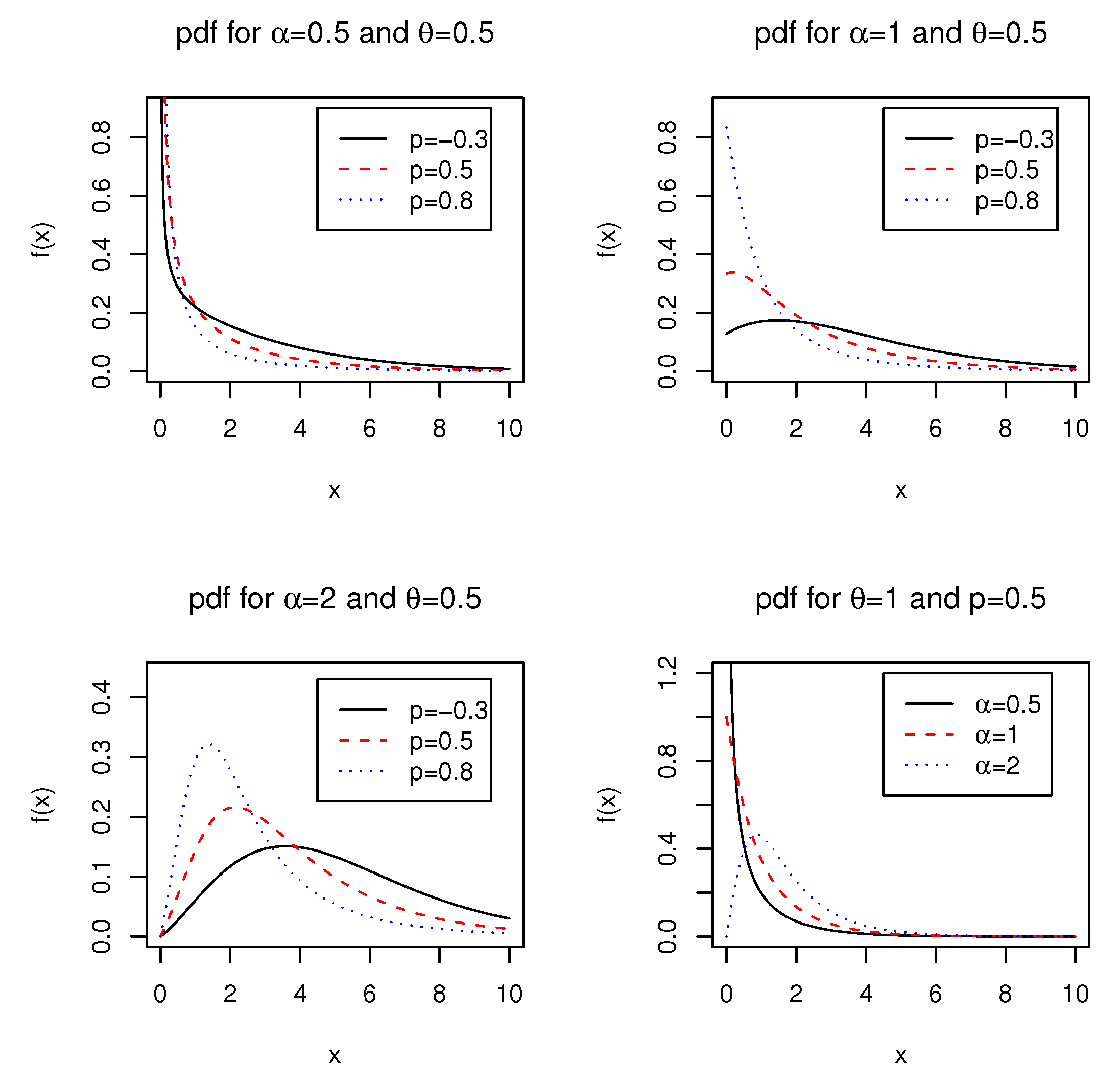
2.1. Probability Density function
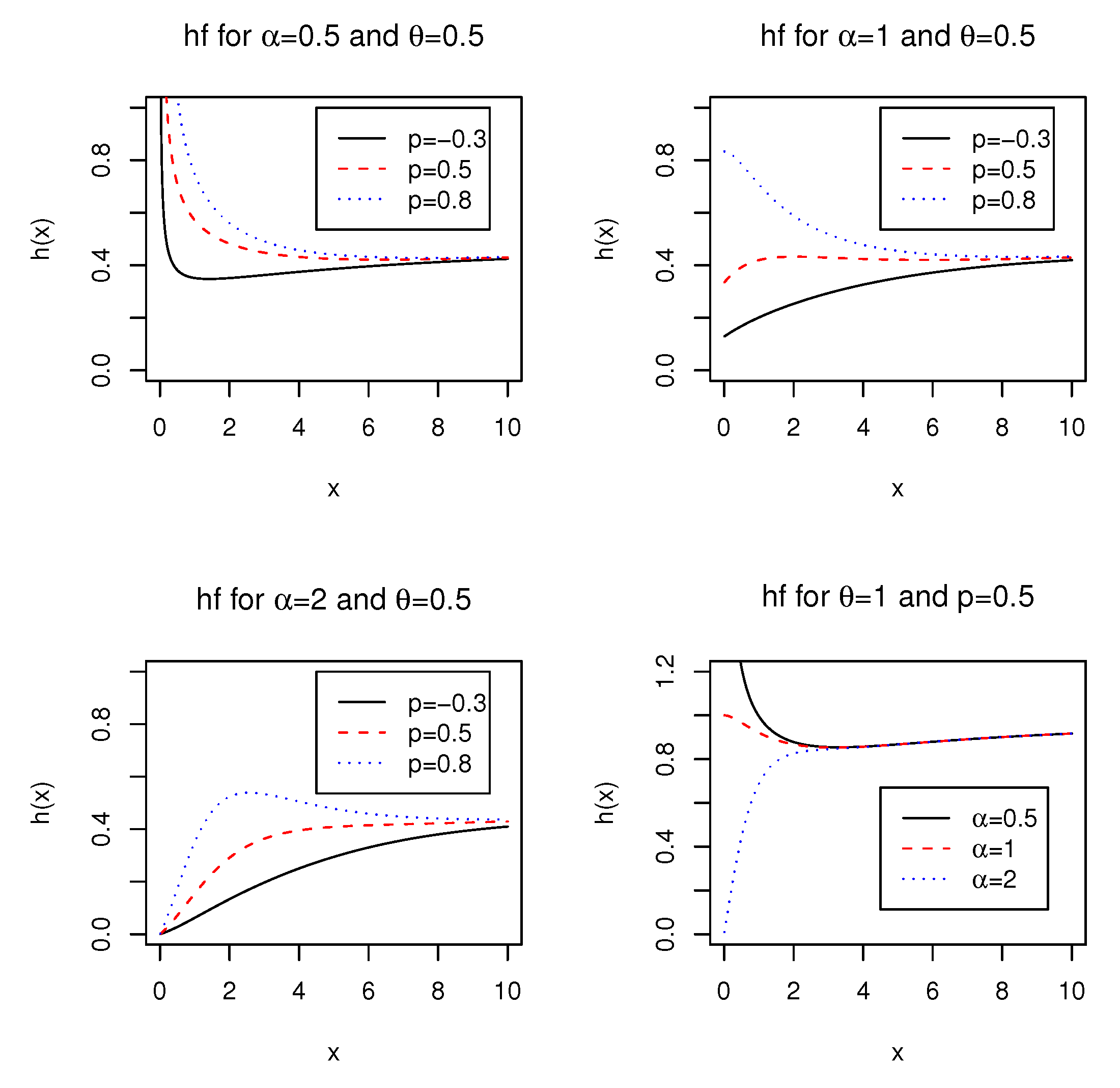
2.2. Hazard Rate Function
2.3. Quantile Function
2.4. Order Statistics
2.5. Moment Properties
2.6. Residual Life Function
2.7. Mean Deviations
2.8. Bonferroni and Lorenz Curves
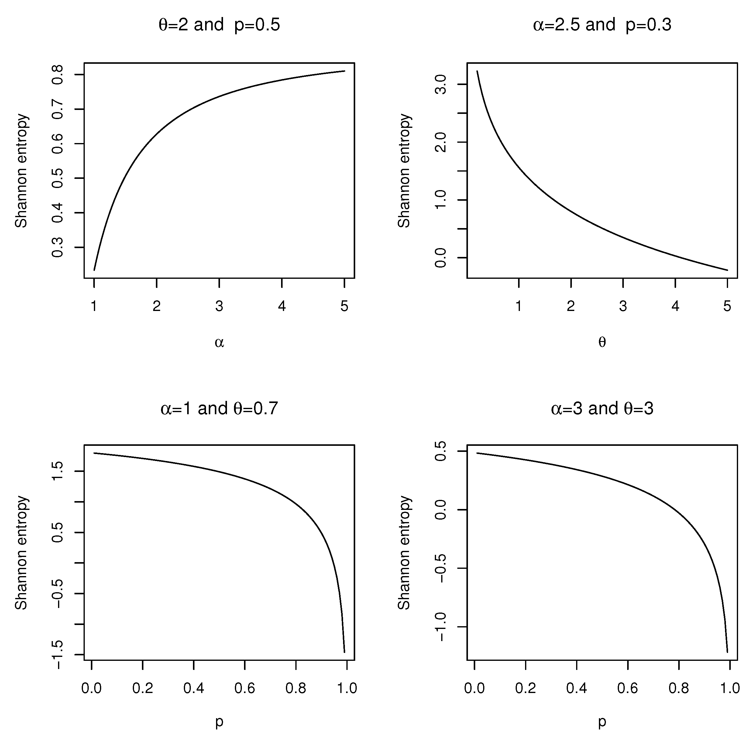
2.9. Entropies
3. Estimation of Parameters
3.1. Maximum Likelihood Estimation
3.2. Expectation-Maximization Algorithm
3.3. Censored Maximum Likelihood Estimation
- is known to have failed at the times ,
- is known to have failed into the interval for ,
- is known to have survived at a time for but not observed any longer.
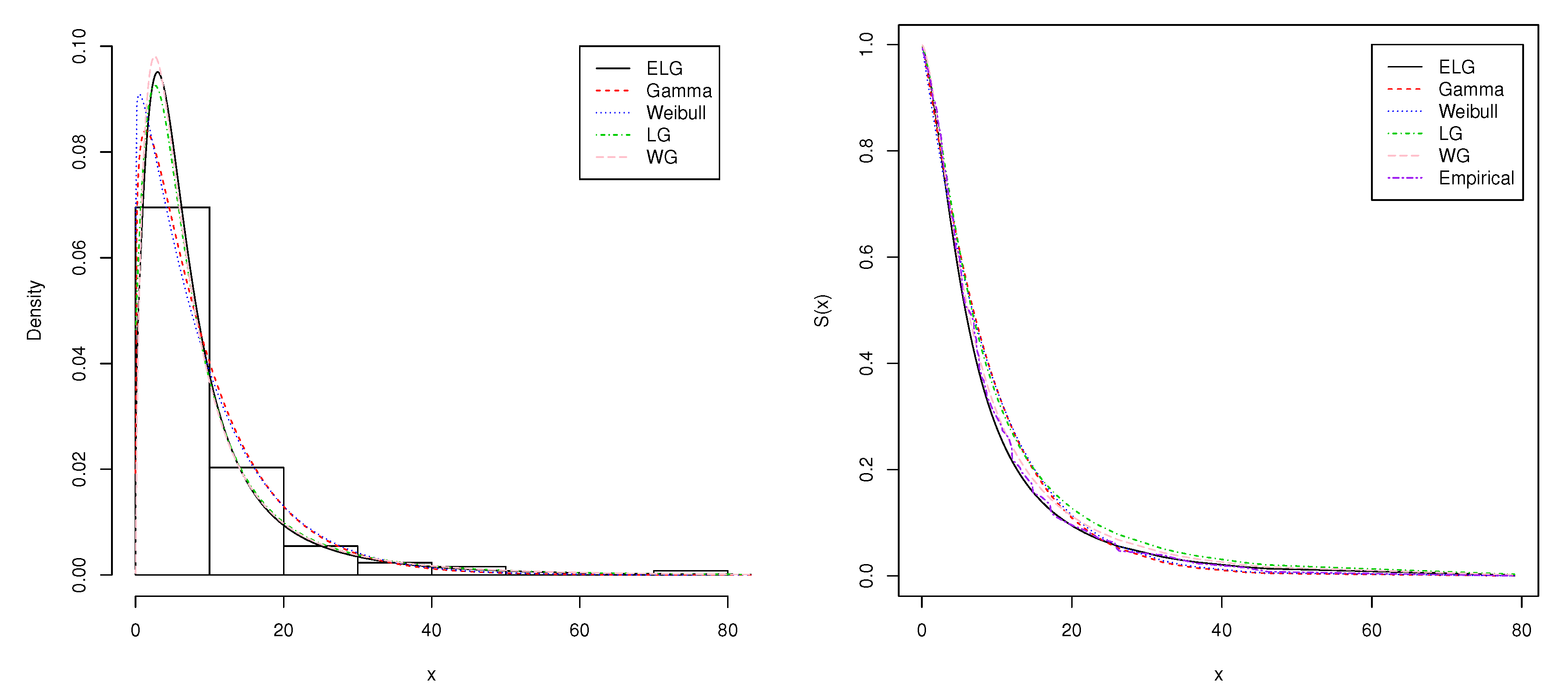
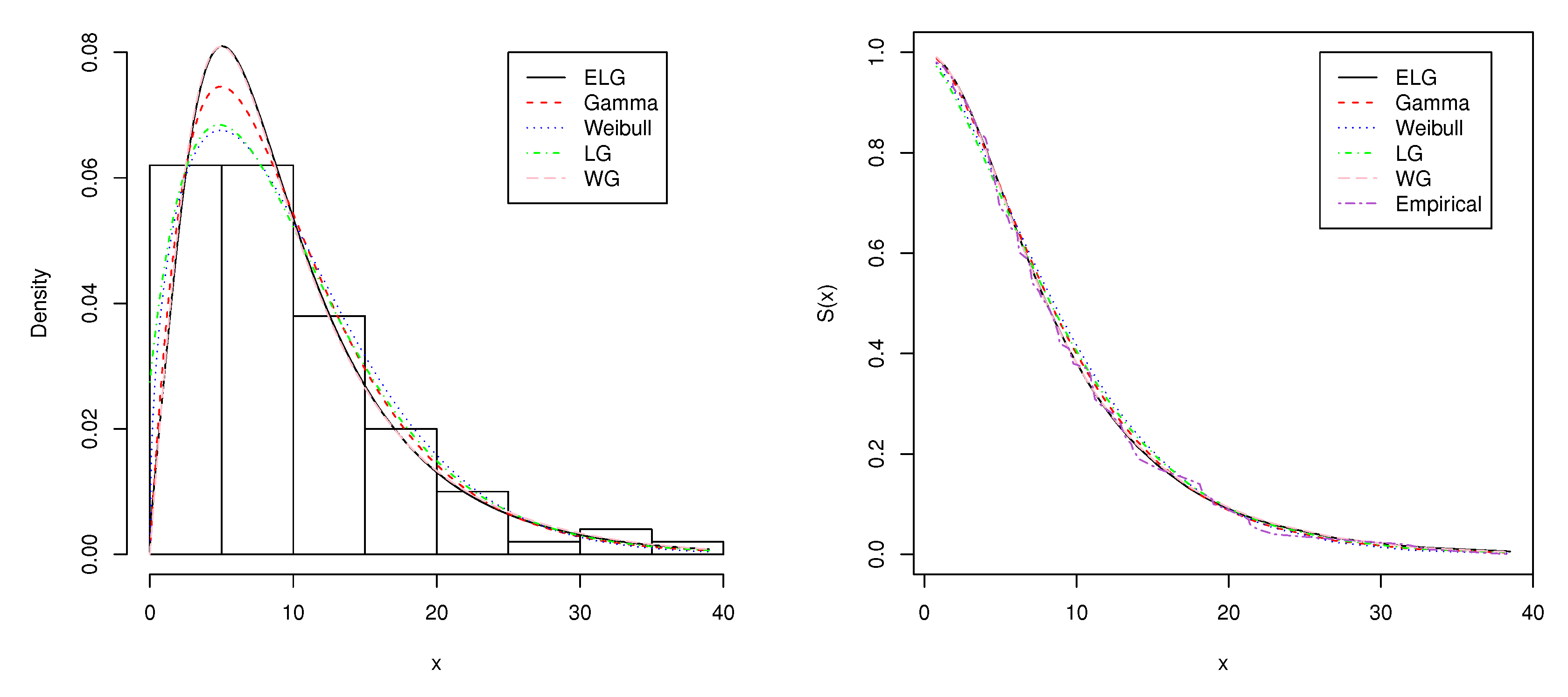
4. Two Real-Data Applications
- (i)
- Gamma
- (ii)
- Weibull
- (iii)
- LG
- (iv)
- WG
5. Concluding Remarks
Author Contributions
Funding
Acknowledgments
Conflicts of Interest
References
- Nadarajah, S.; Cancho, V.; Ortega, E.M. The geometric exponential Poisson distribution. Stat. Methods Appl. 2013, 22, 355–380. [Google Scholar] [CrossRef]
- Conti, M.; Gregori, E.; Panzieri, F. Load distribution among replicated web servers: A QoS-based approach. SIGMETRICS Perform. Eval. Rev. 2000, 27, 12–19. [Google Scholar] [CrossRef]
- Fricker, C.; Gast, N.; Mohamed, H. Mean field analysis for inhomogeneous bike sharing systems. In Proceedings of the DMTCS, Montreal, QC, Canada, 18–22 June 2012; pp. 365–376. [Google Scholar]
- Adamidis, K.; Loukas, S. A lifetime distribution with decreasing failure rate. Stat. Probab. Lett. 1998, 39, 35–42. [Google Scholar] [CrossRef]
- Rezaei, S.; Nadarajah, S.; Tahghighnia, N. A new three-parameter lifetime distribution. Statistics 2013, 47, 835–860. [Google Scholar] [CrossRef]
- Barreto-Souza, W.; de Morais, A.L.; Cordeiro, G.M. The Weibull-geometric distribution. J. Stat. Comput. Simul. 2011, 81, 645–657. [Google Scholar] [CrossRef]
- Pararai, M.; Warahena-Liyanage, G.; Oluyede, B.O. Exponentiated power Lindley-Poisson distribution: Properties and applications. Commun. Stat. Theory Methods 2017, 46, 4726–4755. [Google Scholar] [CrossRef]
- Lindley, D.V. Fiducial distributions and Bayes’ theorem. J. R. Stat. Soc. Ser. B. Methodol. 1958, 20, 102–107. [Google Scholar] [CrossRef]
- Gupta, P.; Singh, B. Parameter estimation of Lindley distribution with hybrid censored data. Int. J. Syst. Assur. Eng. Manag. 2012, 4, 378–385. [Google Scholar] [CrossRef]
- Mazucheli, J.; Achcar, J.A. The Lindley distribution applied to competing risks lifetime data. Comput. Methods Progr. Biomed. 2011, 104, 188–192. [Google Scholar] [CrossRef]
- Zakerzadeh, Y.; Dolati, A. Generalized Lindley distribution. J. Math. Ext. 2009, 3, 13–25. [Google Scholar]
- Ghitany, M.E.; Atieh, B.; Nadarajah, S. Lindley distribution and its application. Math. Comput. Simul. 2008, 78, 493–506. [Google Scholar] [CrossRef]
- Arellano-Valle, R.B.; Contreras-Reyes, J.E.; Stehlík, M. Generalized skew-normal negentropy and its application to fish condition factor time series. Entropy 2017, 19, 528. [Google Scholar] [CrossRef]
- Zakerzadeh, H.; Mahmoudi, E. A new two parameter lifetime distribution: Model and properties. arXiv 2012, arXiv:1204.4248. [Google Scholar]
- Nadarajah, S.; Bakouch, H.S.; Tahmasbi, R. A generalized Lindley distribution. Sankhya B 2011, 73, 331–359. [Google Scholar] [CrossRef]
- Jodrá, P. Computer generation of random variables with lindley or Poisson-Lindley distribution via the lambert W function. Math. Comput. Simul. 2010, 81, 851–859. [Google Scholar] [CrossRef]
- Adler, A. lamW: Lambert-W Function; R package version 1.3.0. 2017. Available online: https://cran.r-project.org/web/packages/lamW/lamW.pdf (accessed on 18 May 2019).
- Leadbetter, M.R.; Lindgren, G.; Rootzén, H. Extremes and Related Properties of Random Sequences and Processes; Springer Series in Statistics; Springer: New York, NY, USA, 1983. [Google Scholar]
- Dempster, A.P.; Laird, N.M.; Rubin, D.B. Maximum likelihood from incomplete data via the EM algorithm. J. R. Stat. Soc. Ser. B (Methodol.) 1977, 39, 1–38. [Google Scholar] [CrossRef]
- Chen, G.; Balakrishnan, N. A general purpose approximate goodness-of-fit test. J. Qual. Technol. 1995, 27, 154–161. [Google Scholar] [CrossRef]
- Lemonte, A.J.; Cordeiro, G.M. An extended Lomax distribution. Statistics 2013, 47, 800–816. [Google Scholar] [CrossRef]
- Wang, M.; Elbatal, I. The modified Weibull geometric distribution. METRON 2015, 73, 303–315. [Google Scholar] [CrossRef]
- Biçer, C. Statistical inference for geometric process with the power Lindley distribution. Entropy 2018, 20, 723. [Google Scholar] [CrossRef]
- Wang, M. A new three-parameter lifetime distribution and associated inference. arXiv 2013, arXiv:1308.4128. [Google Scholar]


| 0.08 | 2.09 | 3.48 | 4.87 | 6.94 | 8.66 | 13.11 | 23.63 | 0.20 | 2.23 |
| 3.52 | 4.98 | 6.97 | 9.02 | 13.29 | 0.40 | 2.26 | 3.57 | 5.06 | 7.09 |
| 9.22 | 13.80 | 25.74 | 0.50 | 2.46 | 3.64 | 5.09 | 7.26 | 9.47 | 14.24 |
| 25.82 | 0.51 | 2.54 | 3.70 | 5.17 | 7.28 | 9.74 | 14.76 | 26.31 | 0.81 |
| 2.62 | 3.82 | 5.32 | 7.32 | 10.06 | 14.77 | 32.15 | 2.64 | 3.88 | 5.32 |
| 7.39 | 10.34 | 14.83 | 34.26 | 0.90 | 2.69 | 4.18 | 5.34 | 7.59 | 10.66 |
| 15.96 | 36.66 | 1.05 | 2.69 | 4.23 | 5.41 | 7.62 | 10.75 | 16.62 | 43.01 |
| 1.19 | 2.75 | 4.26 | 5.41 | 7.63 | 17.12 | 46.12 | 1.26 | 2.83 | 4.33 |
| 5.49 | 7.66 | 11.25 | 17.14 | 79.05 | 1.35 | 2.87 | 5.62 | 7.87 | 11.64 |
| 17.36 | 1.40 | 3.02 | 4.34 | 5.71 | 7.93 | 11.79 | 18.10 | 1.46 | 4.40 |
| 5.85 | 8.26 | 11.98 | 19.13 | 1.76 | 3.25 | 4.50 | 6.25 | 8.37 | 12.02 |
| 2.02 | 3.31 | 4.51 | 6.54 | 8.53 | 12.03 | 20.28 | 2.02 | 3.36 | 6.76 |
| 12.07 | 21.73 | 2.07 | 3.36 | 6.93 | 8.65 | 12.63 | 22.69 |
| Model | Parameters | AIC | BIC | AICc | ||
|---|---|---|---|---|---|---|
| Gamma | = 0.1252 | 830.7356 | 836.4396 | 830.8316 | ||
| Weibull | = 1.0478 | = 9.5607 | 832.1738 | 837.8778 | 832.2698 | |
| LG | = 0.0742 | 823.1859 | 833.742 | 823.2819 | ||
| WG | = 1.6042 | = 0.0286 | = 0.9362 | 826.1842 | 834.7403 | 826.3777 |
| ELG | = 1.0792 | = 0.0699 | = 0.9204 | 824.6214 | 833.1775 | 824.8149 |
| Statistic | ||
|---|---|---|
| Model | ||
| Gamma | 0.11988 | 0.71928 |
| Weibull | 0.13136 | 0.78643 |
| LG | 0.05374 | 0.33827 |
| WG | 0.01493 | 0.09939 |
| ELG | 0.01389 | 0.09498 |
| 0.8 | 0.8 | 1.3 | 1.5 | 1.8 | 1.9 | 1.9 | 2.1 | 2.6 | 2.7 |
| 2.9 | 3.1 | 3.2 | 3.3 | 3.5 | 3.6 | 4.0 | 4.1 | 4.2 | 4.2 |
| 4.3 | 4.3 | 4.4 | 4.4 | 4.6 | 4.7 | 4.7 | 4.8 | 4.9 | 4.9 |
| 5.0 | 5.3 | 5.5 | 5.7 | 5.7 | 6.1 | 6.2 | 6.2 | 6.2 | 6.3 |
| 6.7 | 6.9 | 7.1 | 7.1 | 7.1 | 7.1 | 7.4 | 7.6 | 7.7 | 8.0 |
| 8.2 | 8.6 | 8.6 | 8.6 | 8.8 | 8.8 | 8.9 | 8.9 | 9.5 | 9.6 |
| 9.7 | 9.8 | 10.7 | 10.9 | 11.0 | 11.0 | 11.1 | 11.2 | 11.2 | 11.5 |
| 11.9 | 12.4 | 12.5 | 12.9 | 13.0 | 13.1 | 13.3 | 13.6 | 13.7 | 13.9 |
| 14.1 | 15.4 | 15.4 | 17.3 | 17.3 | 18.1 | 18.2 | 18.4 | 18.9 | 19.0 |
| 19.9 | 20.6 | 21.3 | 21.4 | 21.9 | 23.0 | 27.0 | 31.6 | 33.1 | 38.5 |
| Model | Parameters | AIC | BIC | AICc | ||
|---|---|---|---|---|---|---|
| Gamma | = 0.2033 | 638.6002 | 643.8106 | 638.724 | ||
| Weibull | = 1.4585 | = 10.9553 | 641.4614 | 646.6717 | 641.5851 | |
| LG | = 0.2027 | 641.8269 | 647.0372 | 641.9506 | ||
| WG | = 1.9789 | = 0.0501 | = 0.82132 | 639.9084 | 647.7239 | 640.1584 |
| ELG | = 1.4602 | = 0.1725 | = 0.5385 | 640.3108 | 648.1263 | 640.5608 |
| Statistic | ||
|---|---|---|
| Model | ||
| Gamma | 0.02761 | 0.18225 |
| Weibull | 0.06294 | 0.39624 |
| LG | 0.05374 | 0.33827 |
| WG | 0.01706 | 0.12365 |
| ELG | 0.01801 | 0.12665 |
© 2019 by the authors. Licensee MDPI, Basel, Switzerland. This article is an open access article distributed under the terms and conditions of the Creative Commons Attribution (CC BY) license (http://creativecommons.org/licenses/by/4.0/).
Share and Cite
Peng, B.; Xu, Z.; Wang, M. The Exponentiated Lindley Geometric Distribution with Applications. Entropy 2019, 21, 510. https://doi.org/10.3390/e21050510
Peng B, Xu Z, Wang M. The Exponentiated Lindley Geometric Distribution with Applications. Entropy. 2019; 21(5):510. https://doi.org/10.3390/e21050510
Chicago/Turabian StylePeng, Bo, Zhengqiu Xu, and Min Wang. 2019. "The Exponentiated Lindley Geometric Distribution with Applications" Entropy 21, no. 5: 510. https://doi.org/10.3390/e21050510
APA StylePeng, B., Xu, Z., & Wang, M. (2019). The Exponentiated Lindley Geometric Distribution with Applications. Entropy, 21(5), 510. https://doi.org/10.3390/e21050510