Analysis of Weak Fault in Hydraulic System Based on Multi-scale Permutation Entropy of Fault-Sensitive Intrinsic Mode Function and Deep Belief Network


Abstract
:1. Introduction
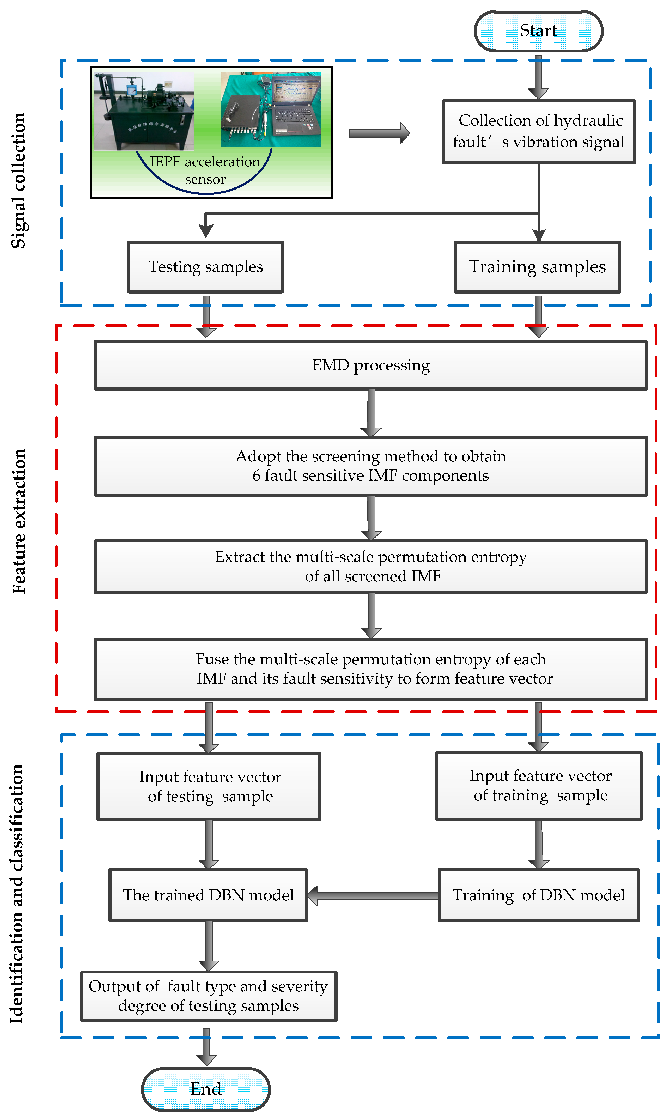
2. Analysis Method
3. Multi-Scale Permutation Entropy
3.1. Permutation Entropy
3.2. Multi-Scale Permutation Entropy
4. Structure and Training of DBN
5. Characteristic Analysis of Leakage Fault with Different Severities
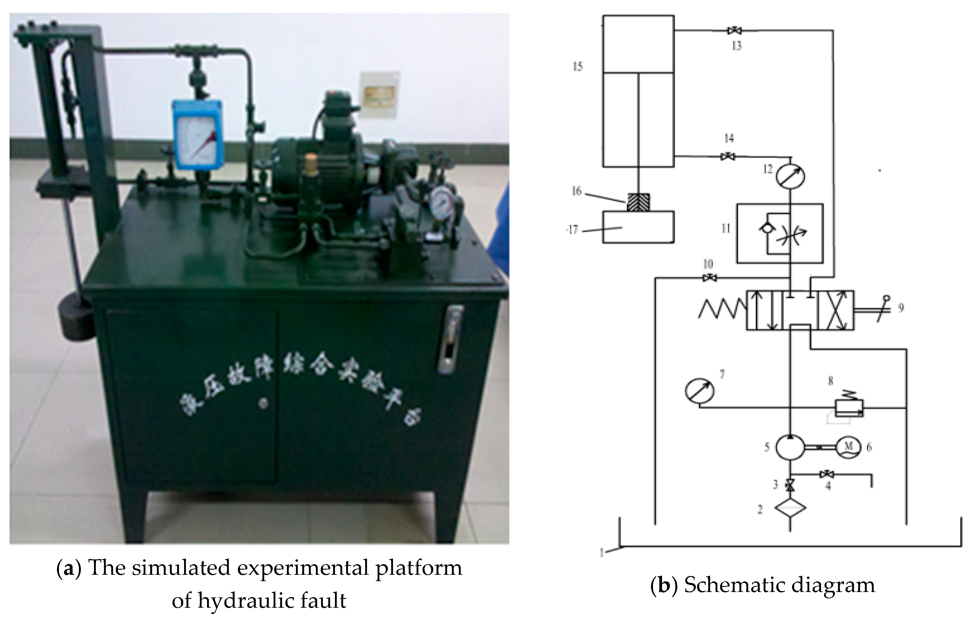
5.1. Comprehensive Experimental Platform of Hydraulic Fault
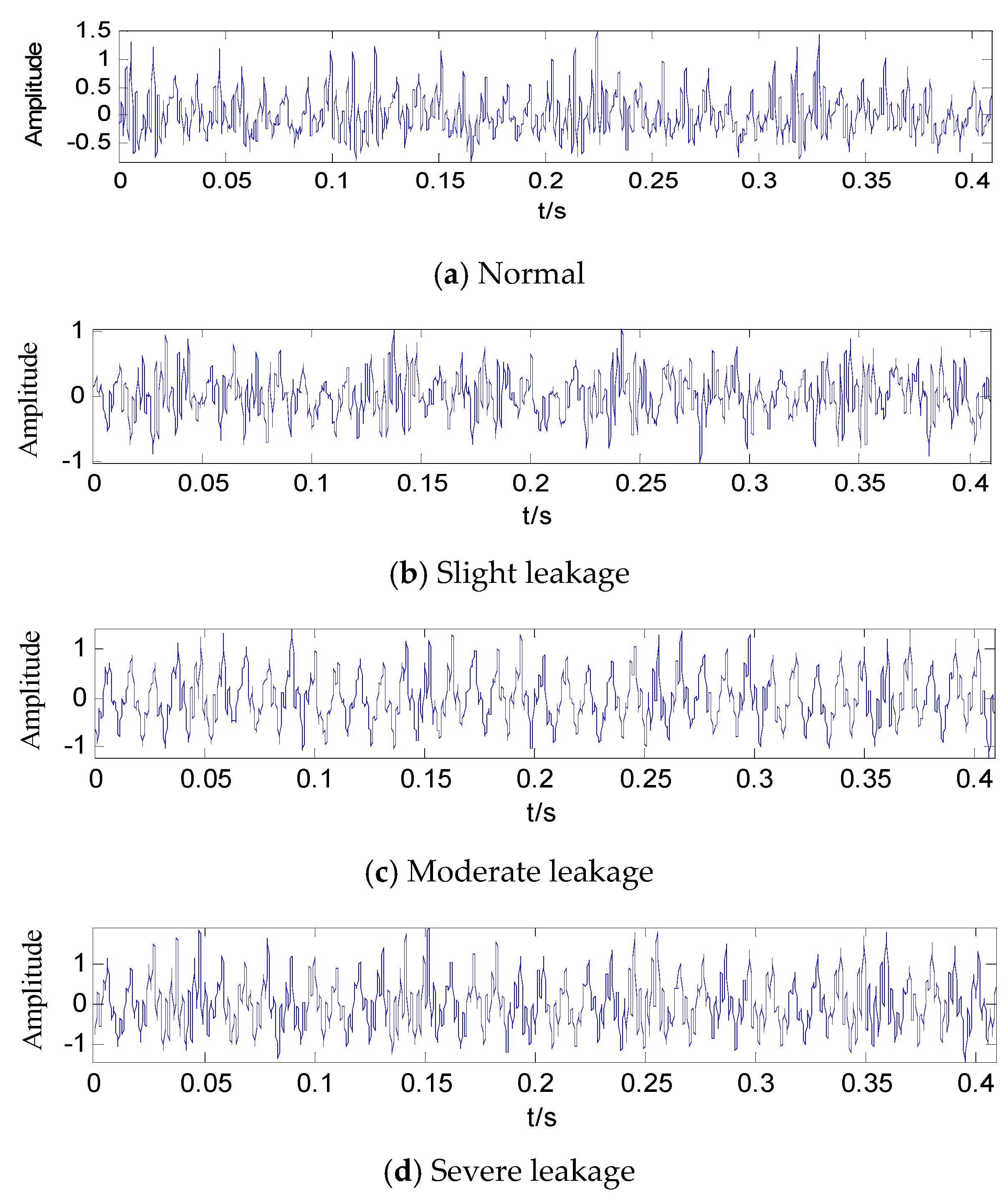
5.2. Leakage Fault Signal
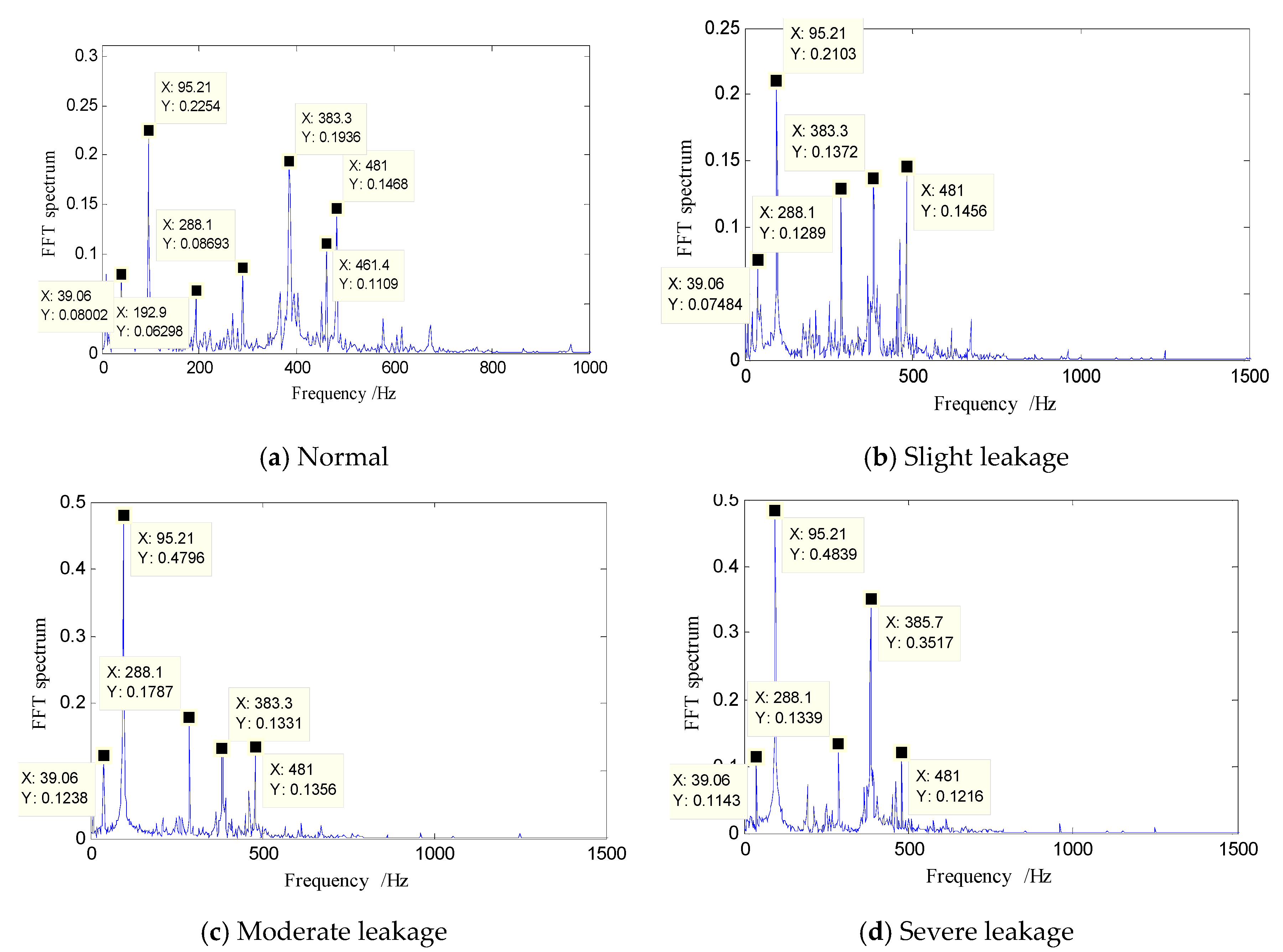
5.3. Spectral Characteristic Analysis of Leakage Fault Signal
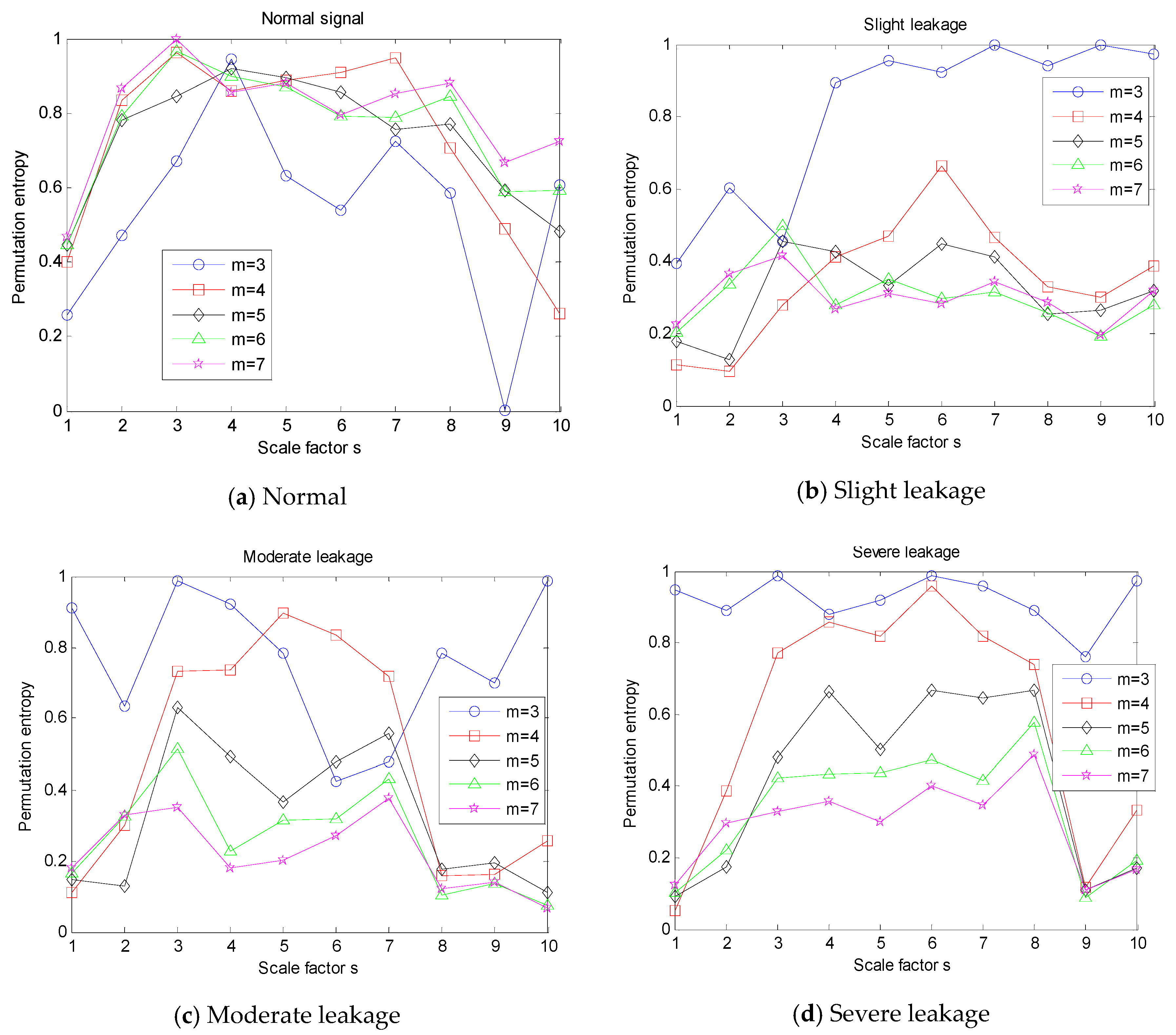
5.4. Influence of Parameter Variation on Multi-Scale Permutation Entropy
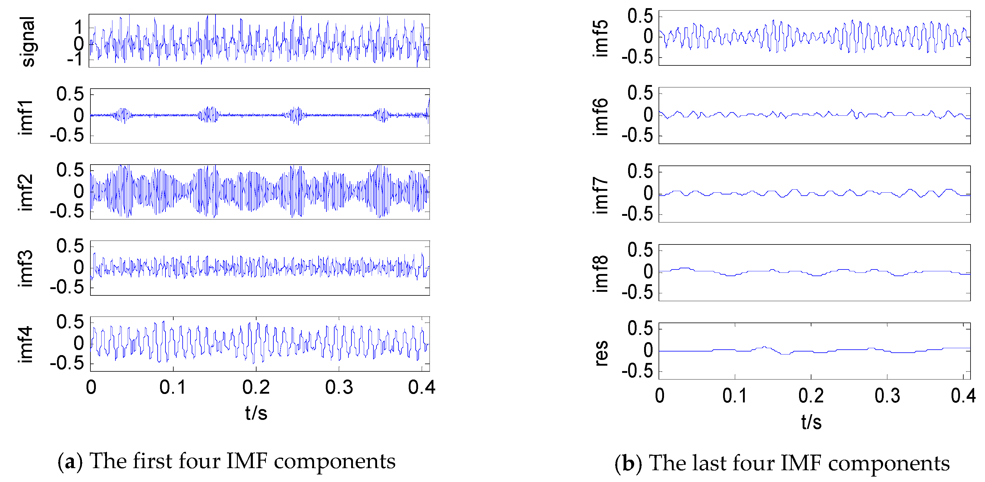
6. Screening of Fault-Sensitive IMF Components
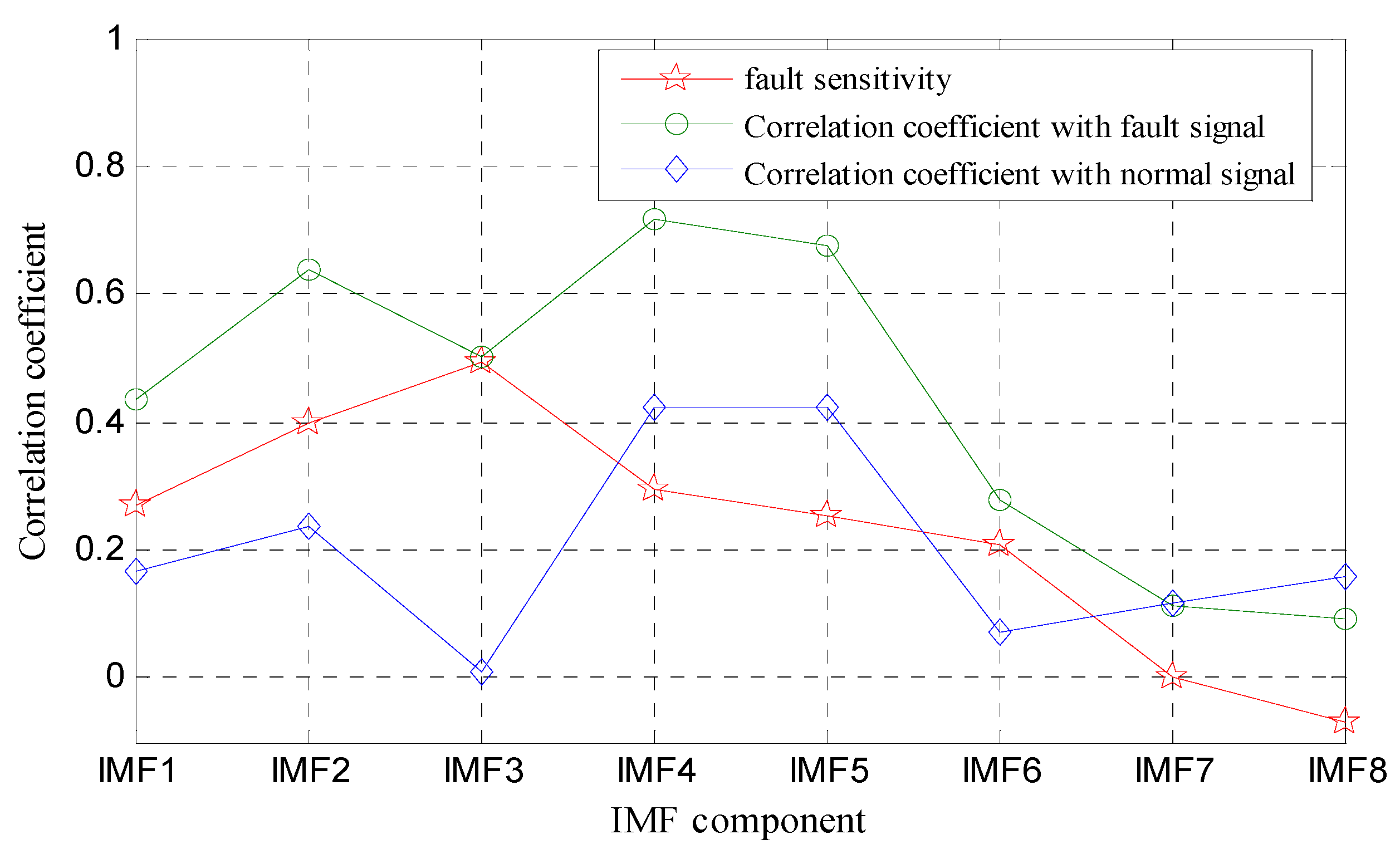
6.1. Calculation of Fault Sensitivity Based on Correlation Analysis
6.2. Screening Process of Fault Sensitive IMF Components
7. Identification and Analysis of Leakage Faults
7.1. Feature Extraction Based on Multi-Scale Permutation Entropy of Fault-Sensitive IMF
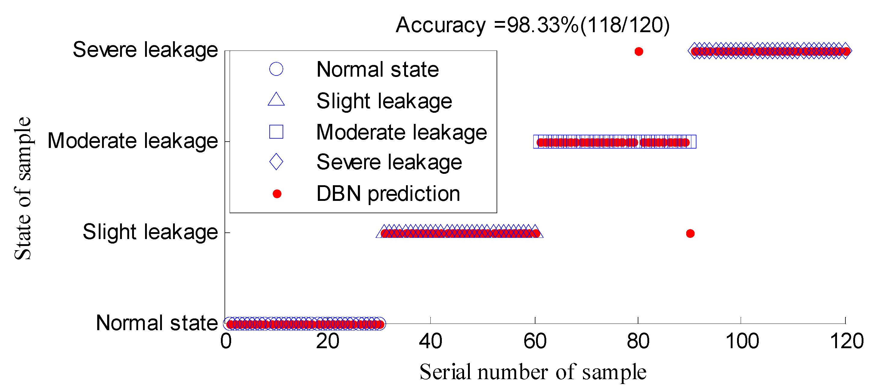
7.2. DBN Identification of Leakage Fault
8. Conclusions
Author Contributions
Acknowledgments
Conflicts of Interest
References
- Zeng, D.; Zhou, D.; Tan, C.; Jiang, B. Research on Model-Based Fault Diagnosis for a Gas Turbine Based on Transient Performance. Appl. Sci. 2018, 8, 148. [Google Scholar] [CrossRef]
- Wang, Y.; Xu, G.; Liang, L.; Jiang, K. Detection of weak transient signals based on wavelet packet transform and manifold learning for rolling element bearing fault diagnosis. Mech. Syst. Signal Process. 2015, 55, 259–276. [Google Scholar] [CrossRef]
- Bustos, A.; Rubio, H.; Castejón, C.; García-Prada, J.C. EMD-Based Methodology for the Identification of a High-Speed Train Running in a Gear Operating State. Sensors 2018, 18, 793. [Google Scholar] [CrossRef]
- Jiang, W.; Zhang, Y.; Wang, H. Hydraulic Pump Fault Diagnosis Method Based on Lyapunov Exponent Analysis. Mach. Tool Hydraul. 2008, 36, 183–185. [Google Scholar]
- Vasquez, S.; Kinnaert, M.; Pintelon, R. Active Fault Diagnosis on a Hydraulic Pitch System Based on Frequency-Domain Identification. IEEE Trans. Contr. Syst. Trans. 2017, 5, 1–16. [Google Scholar] [CrossRef]
- Jiang, W.; Zhou, J.; Zhu, Y.; Cui, X. Experimental Research on Sensitive Characteristic Parameter Selection of Hydraulic Cylinder Internal Leakage Fault. Chin. Hydraul. Pneum. 2014, 3, 119–124. [Google Scholar]
- Yasir, M.N.; Koh, B.H. Data Decomposition Techniques with Multi-Scale Permutation Entropy Calculations for Bearing Fault Diagnosis. Sensors 2018, 18, 1278. [Google Scholar] [CrossRef] [PubMed]
- Ju, B.; Zhang, H.; Liu, Y.; Liu, F.; Lu, S.; Dai, Z. A Feature Extraction Method Using Improved Multi-Scale Entropy for Rolling Bearing Fault Diagnosis. Entropy 2018, 20, 212. [Google Scholar] [CrossRef]
- Chen, J.; Tang, J. Feature extraction of rolling bearing’s weak fault based on POVMD and spectrum auto-correlation analysis. J. Electron. Meas. Instrum. 2018, 4, 13–20. [Google Scholar]
- Wang, H.; Chen, J.; Dong, G. Feature extraction of rolling bearing’s early weak fault based on EEMD and tunable Q-factor wavelet transform. Mech. Syst. Signal Process. 2014, 48, 103–119. [Google Scholar] [CrossRef]
- Yu, J.; Liu, H. Sparse Coding Shrinkage in Intrinsic Time-Scale Decomposition for Weak Fault Feature Extraction of Bearings. IEEE Trans. Instrum. Meas. 2018, 67, 1–14. [Google Scholar] [CrossRef]
- Liu, X.; Liu, H.; Yang, J. Improving the bearing fault diagnosis efficiency by the adaptive stochastic resonance in a new nonlinear system. Mech. Syst. Signal Process. 2017, 96, 58–76. [Google Scholar] [CrossRef]
- Yu, J.; Lv, J. Weak Fault Feature Extraction of Rolling Bearings Using Local Mean Decomposition-Based Multilayer Hybrid Denoising. IEEE Trans. Instrum. Meas. 2017, 66, 3148–3159. [Google Scholar] [CrossRef]
- Yang, Q.; Mei, J.; Xiao, J.; Zhang, L.; Xiao, Y. Weak fault feature extraction for bearings based on an order cepstrum enhanced with Teager energy operator. J. Vib. Shock 2015, 34, 1–5. [Google Scholar]
- Wang, Y.K.; Li, H.R.; Xu, B.H. Faint Fault Feature Extraction of Hydraulic Pump Based on Adaptive EEMD-Enhancement Factor. Mach. Tool Hydraul. 2014, 19, 184–190. [Google Scholar]
- Mustapha, O.; Lefebvre, D.; Khalil, M.; Hoblos, G.; Chafouk, H. Fault detection algorithm using DCS method combined with filters bank derived from the wavelet transform. Int. J. Innov. Comput. Inf. Control 2009, 5, 1313–1327. [Google Scholar]
- Ben, A.J.; Fnaiech, N.; Saidi, L. Application of empirical mode decomposition and artificial neural network for automatic bearing fault diagnosis based on vibration signals. Appl. Acoust. 2015, 89, 16–27. [Google Scholar] [CrossRef]
- Fu, X.; Liu, B.; Zhang, Y.; Lian, L. Fault diagnosis of hydraulic system in large forging hydraulic press. Measurement 2014, 49, 390–396. [Google Scholar] [CrossRef]
- Zhao, X.X.; Zhang, S.; Zhou, C.L. Experimental study of hydraulic cylinder leakage and fault feature extraction based on wavelet packet analysis. Comput. Fluids 2015, 106, 33–40. [Google Scholar] [CrossRef]
- Hinton, G.; Osindero, S.; Teh, Y. A fast learning algorithm for deep belief nets. Neural Comput. 2014, 18, 1527–1554. [Google Scholar] [CrossRef]
- Hinton, G. A practical guide to training restricted Boltzmann machines. Momentum 2010, 9, 1–21. [Google Scholar]
- Bandt, C.; Pompe, B. Permutation Entropy: A Natural Complexity Measure for Time Series. Phys. Rev. Lett. 2002, 88, 174102. [Google Scholar] [CrossRef] [PubMed]
- Aziz, W.; Arif, M. Multiscale Permutation Entropy of Physiological Time Series. In Proceedings of the IEEE International Multi-Topic Conference, Karachi, Pakistan, 24–25 December 2005; pp. 1–6. [Google Scholar]
- Bengio, Y.; Lamblin, P.; Popovici, D. Greedy layer-wise training of deep networks. Adv. Neur. Inform. Process. Syst. 2007, 19, 153–160. [Google Scholar]
- Zheng, J.D.; Cheng, J.S.; Yang, Y. Multi-scale permutation entropy and its applications to rolling bearing fault diagnosis. China Mech. Eng. 2013, 24, 2641–2646. [Google Scholar]


| Sample Type | Serial Number | Feature Vector | |||||||||||||||||
|---|---|---|---|---|---|---|---|---|---|---|---|---|---|---|---|---|---|---|---|
| Multi-Scale Permutation | |||||||||||||||||||
| … | |||||||||||||||||||
| 1 | 2 | 3 | 4 | 5 | 6 | 7 | 8 | 9 | 10 | … | |||||||||
| Normal State | 1 | 0.64 | 0.18 | 0.45 | 0.49 | 0.96 | 0.62 | 0.80 | 0.99 | 0.47 | 0.97 | 0.95 | 0.50 | 0.98 | 0.90 | 0.89 | 0.40 | … | |
| 2 | 0.53 | 0.18 | 0.35 | 0.39 | 0.67 | 0.53 | 0.93 | 0.99 | 0.52 | 0.89 | 0.83 | 0.38 | 0.60 | 0.82 | 0.97 | 0.49 | |||
| ⋮ | ⋮ | ⋮ | … | ||||||||||||||||
| 100 | 0.69 | 0.55 | 0.64 | 0.14 | 0.27 | 0.26 | 0.86 | 0.95 | 0.33 | 0.91 | 0.65 | 0.24 | 0.64 | 0.42 | 0.68 | 0.55 | |||
| Slight Leakage | 1 | 0.83 | 0.24 | 0.17 | 0.57 | 0.89 | 0.53 | 0.76 | 0.99 | 0.63 | 0.97 | 0.58 | 0.31 | 0.79 | 0.67 | 0.66 | 0.00 | ||
| 2 | 0.47 | 0.13 | 0.45 | 0.35 | 0.48 | 0.17 | 0.93 | 1.00 | 0.24 | 0.92 | 0.96 | 0.21 | 1.00 | 0.95 | 0.91 | 0.69 | |||
| ⋮ | ⋮ | ⋮ | … | ⋮ | |||||||||||||||
| 100 | 0.48 | 0.37 | 0.69 | 0.32 | 0.48 | 0.32 | 0.96 | 1.00 | 0.61 | 0.95 | 0.87 | 0.45 | 0.78 | 0.93 | 0.88 | 0.64 | |||
| Moderate Leakage | 1 | 0.43 | 0.53 | 0.84 | 0.50 | 0.44 | 0.22 | 0.80 | 0.96 | 0.00 | 0.33 | 0.76 | 0.29 | 0.79 | 0.86 | 0.72 | 0.61 | ||
| 2 | 0.29 | 0.10 | 0.37 | 0.28 | 0.25 | 0.15 | 0.98 | 1.00 | 0.24 | 0.91 | 0.48 | 0.04 | 0.63 | 0.95 | 0.98 | 0.64 | |||
| ⋮ | ⋮ | ⋮ | … | ||||||||||||||||
| 100 | 0.14 | 0.17 | 0.28 | 0.30 | 0.36 | 0.05 | 0.98 | 0.97 | 0.31 | 0.73 | 0.88 | 0.04 | 0.83 | 0.84 | 0.86 | 0.97 | |||
| Severe Leakage | 1 | 0.25 | 0.80 | 0.41 | 0.20 | 0.06 | 0.07 | 0.96 | 1.00 | 0.43 | 0.91 | 0.92 | 0.14 | 0.70 | 0.70 | 0.99 | 0.44 | ||
| 2 | 0.43 | 0.88 | 0.37 | 0.13 | 0.32 | 0.01 | 0.77 | 0.99 | 0.20 | 0.98 | 0.87 | 0.17 | 0.78 | 0.51 | 1.00 | 0.68 | |||
| ⋮ | ⋮ | ⋮ | … | ||||||||||||||||
| 100 | 0.26 | 0.85 | 0.27 | 0.28 | 0.35 | 0.30 | 0.15 | 0.00 | 0.13 | 0.00 | 0.11 | 0.10 | 0.38 | 0.20 | 0.98 | 0.71 | … | ||
| Number | Feature Extraction | Classifier | Recognition Rate |
|---|---|---|---|
| 1 | multi-scale permutation entropy of all IMFs | SVM | 89.16% (107/120) |
| 2 | multi-scale permutation entropy of all IMFs | DBN | 90% (108/120) |
| 3 | multi-scale permutation entropy of fault-sensitive IMFs | SVM | 95.83% (115/120) |
| 4 | multi-scale permutation entropy of fault-sensitive IMFs | DBN | 98.33% (118/120) |
© 2019 by the authors. Licensee MDPI, Basel, Switzerland. This article is an open access article distributed under the terms and conditions of the Creative Commons Attribution (CC BY) license (http://creativecommons.org/licenses/by/4.0/).
Share and Cite
Huang, J.; Wang, X.; Wang, D.; Wang, Z.; Hua, X. Analysis of Weak Fault in Hydraulic System Based on Multi-scale Permutation Entropy of Fault-Sensitive Intrinsic Mode Function and Deep Belief Network. Entropy 2019, 21, 425. https://doi.org/10.3390/e21040425
Huang J, Wang X, Wang D, Wang Z, Hua X. Analysis of Weak Fault in Hydraulic System Based on Multi-scale Permutation Entropy of Fault-Sensitive Intrinsic Mode Function and Deep Belief Network. Entropy. 2019; 21(4):425. https://doi.org/10.3390/e21040425
Chicago/Turabian StyleHuang, Jie, Xinqing Wang, Dong Wang, Zhiwei Wang, and Xia Hua. 2019. "Analysis of Weak Fault in Hydraulic System Based on Multi-scale Permutation Entropy of Fault-Sensitive Intrinsic Mode Function and Deep Belief Network" Entropy 21, no. 4: 425. https://doi.org/10.3390/e21040425
APA StyleHuang, J., Wang, X., Wang, D., Wang, Z., & Hua, X. (2019). Analysis of Weak Fault in Hydraulic System Based on Multi-scale Permutation Entropy of Fault-Sensitive Intrinsic Mode Function and Deep Belief Network. Entropy, 21(4), 425. https://doi.org/10.3390/e21040425