A Reference-Free Lossless Compression Algorithm for DNA Sequences Using a Competitive Prediction of Two Classes of Weighted Models


Abstract
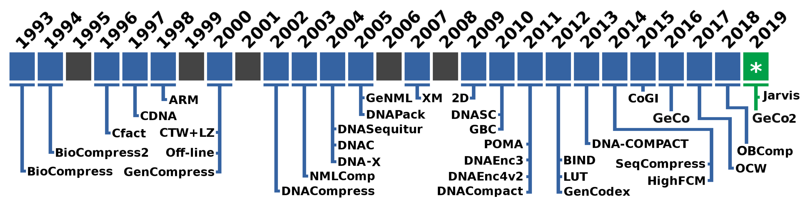
1. Introduction
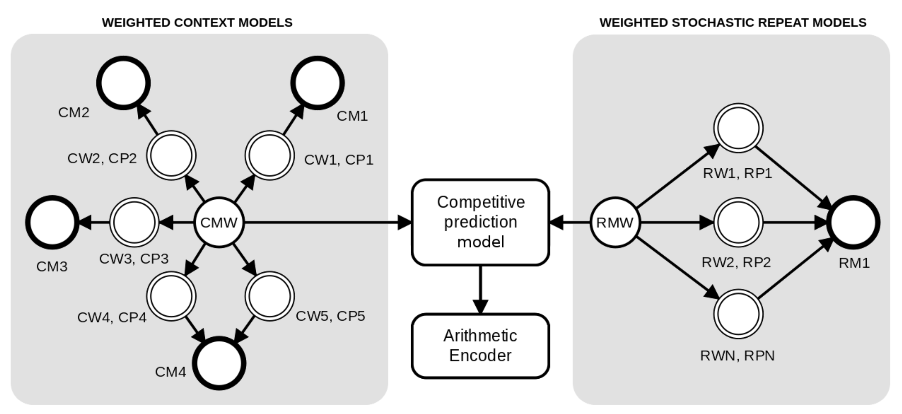
2. Method
2.1. Weighted Context Models
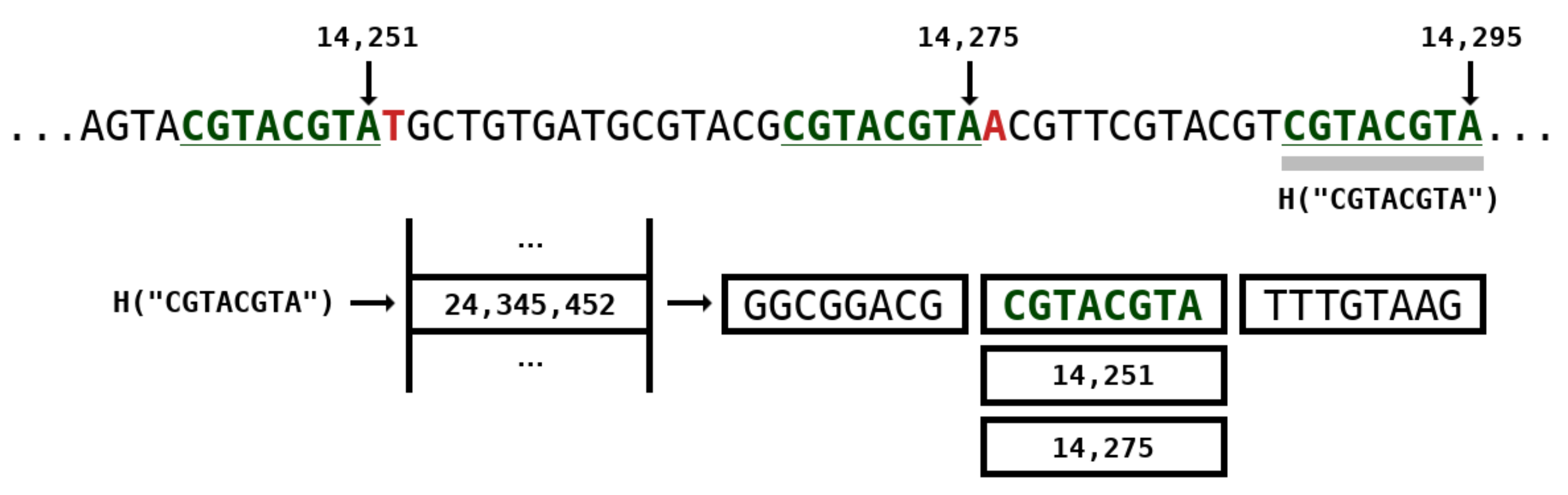
2.2. Weighted Stochastic Repeat Models
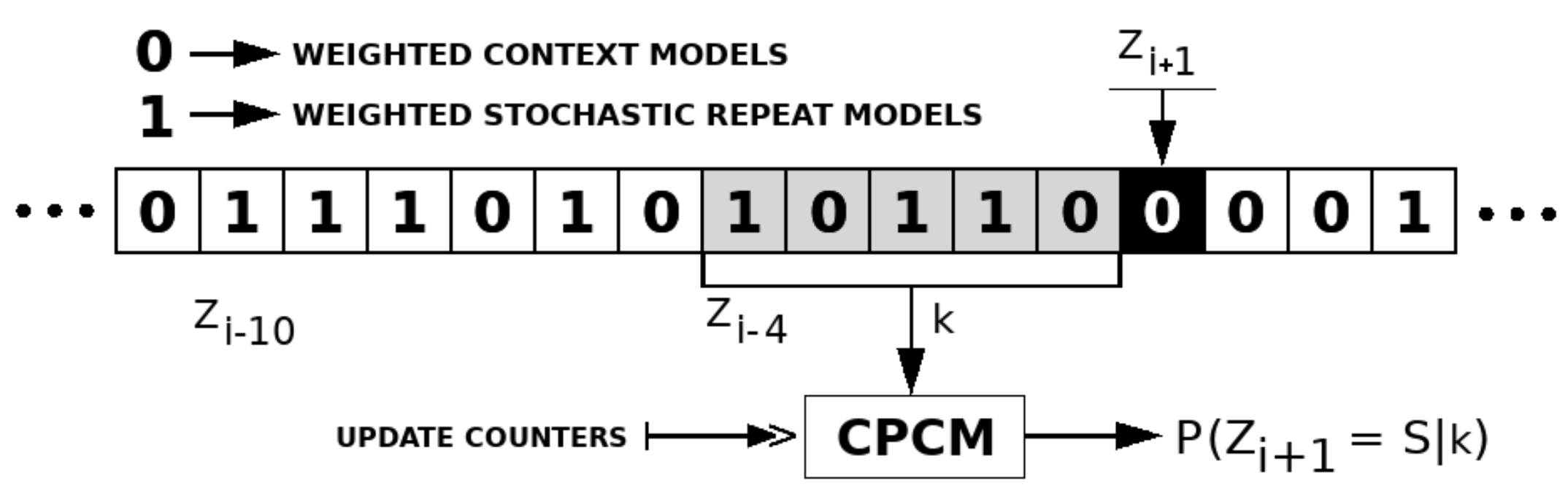
2.3. Competitive Prediction Context Model
2.4. Decompression
2.5. Implementation
3. Results
4. Conclusions
Author Contributions
Funding
Acknowledgments
Conflicts of Interest
Abbreviations
| AeCa | Aeropyrum camini—archaea |
| AgPh | Aggregatibacter phage S1249—phage virus |
| BPS | Bits per symbol |
| BuEb | Bundibugyo ebolavirus—virus |
| CPCM | Competitive prediction context model |
| CTW | Context tree weighting |
| DaRe | Danio rerio—fish |
| DrMe | Drosophila miranda—fly |
| EnIn | Entamoeba invadens—amoebozoa |
| EsCo | Escherichia coli—bacteria |
| GaGa | Gallus gallus—chicken |
| GeCo | Genomic Compressor (tool) |
| GPU | Graphical Processing Unit |
| HaHi | Haloarcula hispanica—archaea |
| HePy | Helicobacter pylori—bacteria |
| HoSa | Homo sapiens—human |
| LUT | Look Up Table |
| NC | Normalized Compression |
| OrSa | Oriza sativa—plant |
| OS | Operating System |
| PlFa | Plasmodium falciparum–protozoan |
| RAM | Random Access Memory |
| RLE | Run Length Encoding |
| ScPo | Schizosaccharomyces pombe—fungi |
| TB | TeraByte |
| XM | eXpert-Model |
| YeMi | Yellowstone lake—mimivirus |
References
- Schatz, M.C.; Langmead, B. The DNA data deluge. IEEE Spectrum 2013, 50, 28–33. [Google Scholar] [CrossRef] [PubMed][Green Version]
- Mardis, E.R. DNA sequencing technologies: 2006–2016. Nat. Protocols 2017, 12, 213. [Google Scholar] [CrossRef] [PubMed]
- Marco, D. Metagenomics: Theory, Methods and Applications; Horizon Scientific Press: Poole, UK, 2010. [Google Scholar]
- Duggan, A.T.; Perdomo, M.F.; Piombino-Mascali, D.; Marciniak, S.; Poinar, D.; Emery, M.V.; Buchmann, J.P.; Duchêne, S.; Jankauskas, R.; Humphreys, M.; et al. 17th century variola virus reveals the recent history of smallpox. Curr. Biol. 2016, 26, 3407–3412. [Google Scholar] [CrossRef] [PubMed]
- Weber, W.; Fussenegger, M. Emerging biomedical applications of synthetic biology. Nat. Rev. Genet. 2012, 13, 21. [Google Scholar] [CrossRef] [PubMed]
- Marciniak, S.; Perry, G.H. Harnessing ancient genomes to study the history of human adaptation. Nat. Rev. Genet. 2017, 18, 659. [Google Scholar] [CrossRef] [PubMed]
- Stephens, Z.D.; Lee, S.Y.; Faghri, F.; Campbell, R.H.; Zhai, C.; Efron, M.J.; Iyer, R.; Schatz, M.C.; Sinha, S.; Robinson, G.E. Big data: Astronomical or genomical? PLoS Biol. 2015, 13, e1002195. [Google Scholar] [CrossRef]
- Deorowicz, S.; Grabowski, S. Compression of DNA sequence reads in FASTQ format. Bioinformatics 2011, 27, 860–862. [Google Scholar] [CrossRef]
- Hanus, P.; Dingel, J.; Chalkidis, G.; Hagenauer, J. Compression of whole genome alignments. IEEE Trans. Inf. Theory 2010, 56, 696–705. [Google Scholar] [CrossRef]
- Matos, L.M.O.; Pratas, D.; Pinho, A.J. A compression model for DNA multiple sequence alignment blocks. IEEE Trans. Inf. Theory 2013, 59, 3189–3198. [Google Scholar] [CrossRef]
- Mohammed, M.H.; Dutta, A.; Bose, T.; Chadaram, S.; Mande, S.S. DELIMINATE—A fast and efficient method for loss-less compression of genomic sequences. Bioinformatics 2012, 28, 2527–2529. [Google Scholar] [CrossRef]
- Pinho, A.J.; Pratas, D. MFCompress: A compression tool for fasta and multi-fasta data. Bioinformatics 2013, 30, 117–118. [Google Scholar] [CrossRef] [PubMed]
- Grabowski, S.; Deorowicz, S.; Roguski, Ł. Disk-based compression of data from genome sequencing. Bioinformatics 2015, 31, 1389–1395. [Google Scholar] [CrossRef] [PubMed]
- Hach, F.; Numanagić, I.; Alkan, C.; Sahinalp, S.C. SCALCE: Boosting sequence compression algorithms using locally consistent encoding. Bioinformatics 2012, 28, 3051–3057. [Google Scholar] [CrossRef] [PubMed]
- Layer, R.M.; Kindlon, N.; Karczewski, K.J.; Consortium, E.A.; Quinlan, A.R. Efficient genotype compression and analysis of large genetic-variation data sets. Nat. Methods 2016, 13, 63. [Google Scholar] [CrossRef]
- Bonfield, J.K.; Mahoney, M.V. Compression of FASTQ and SAM format sequencing data. PLoS ONE 2013, 8, e59190. [Google Scholar] [CrossRef]
- Wang, R.; Bai, Y.; Chu, Y.S.; Wang, Z.; Wang, Y.; Sun, M.; Li, J.; Zang, T.; Wang, Y. DeepDNA: A hybrid convolutional and recurrent neural network for compressing human mitochondrial genomes. In Proceedings of the 2018 IEEE International Conference on Bioinformatics and Biomedicine (BIBM), Madrid, Spain, 3–6 December 2018; pp. 270–274. [Google Scholar]
- Benoit, G.; Lemaitre, C.; Lavenier, D.; Drezen, E.; Dayris, T.; Uricaru, R.; Rizk, G. Reference-free compression of high throughput sequencing data with a probabilistic de Bruijn graph. BMC Bioinform. 2015, 16, 288. [Google Scholar] [CrossRef]
- Ochoa, I.; Li, H.; Baumgarte, F.; Hergenrother, C.; Voges, J.; Hernaez, M. AliCo: A new efficient representation for SAM files. In Proceedings of the 2019 Data Compression Conference (DCC), Snowbird, UT, USA, 26–29 March 2019; pp. 93–102. [Google Scholar]
- Zhang, C.; Ochoa, I. VEF: A Variant Filtering tool based on Ensemble methods. bioRxiv 2019, 540286. [Google Scholar] [CrossRef]
- Chandak, S.; Tatwawadi, K.; Ochoa, I.; Hernaez, M.; Weissman, T. SPRING: A next-generation compressor for FASTQ data. Bioinformatics 2018, 35, 2674–2676. [Google Scholar] [CrossRef]
- Holley, G.; Wittler, R.; Stoye, J.; Hach, F. Dynamic alignment-free and reference-free read compression. J. Comput. Biol. 2018, 25, 825–836. [Google Scholar] [CrossRef]
- Kumar, S.; Agarwal, S. WBMFC: Efficient and Secure Storage of Genomic Data. Pertanika J. Sci. Technol. 2018, 26, 4. [Google Scholar]
- Dougherty, E.R.; Shmulevich, I.; Chen, J.; Wang, Z.J. (Eds.) Genomic Signal Processing and Statistics; Hindawi Publishing Corporation: London, UK, 2005. [Google Scholar]
- Grumbach, S.; Tahi, F. Compression of DNA sequences. In Proceedings of the Data Compression Conference (DCC 1993), Snowbird, UT, USA, 30 March–2 April 1993; pp. 340–350. [Google Scholar]
- Hernaez, M.; Pavlichin, D.; Weissman, T.; Ochoa, I. Genomic Data Compression. Annu. Rev. Biomed. Data Sci. 2019, 2, 19–37. [Google Scholar] [CrossRef]
- Rieseberg, L.H. Chromosomal rearrangements and speciation. Trends Ecol. Evol. 2001, 16, 351–358. [Google Scholar] [CrossRef]
- Roeder, G.S.; Fink, G.R. DNA rearrangements associated with a transposable element in yeast. Cell 1980, 21, 239–249. [Google Scholar] [CrossRef]
- Harris, K. Evidence for recent, population-specific evolution of the human mutation rate. Proc. Natl. Acad. Sci. USA 2015, 112, 3439–3444. [Google Scholar] [CrossRef] [PubMed]
- Jeong, C.; di Rienzo, A. Adaptations to local environments in modern human populations. Curr. Opin. Genet. Dev. 2014, 29, 1–8. [Google Scholar] [CrossRef] [PubMed]
- Beres, S.; Kachroo, P.; Nasser, W.; Olsen, R.; Zhu, L.; Flores, A.; de la Riva, I.; Paez-Mayorga, J.; Jimenez, F.; Cantu, C.; et al. Transcriptome remodeling contributes to epidemic disease caused by the human pathogen Streptococcus pyogenes. mBio 2016, 7, e00403-16. [Google Scholar] [CrossRef]
- Fumagalli, M.; Sironi, M. Human genome variability, natural selection and infectious diseases. Curr. Opin. Immunol. 2014, 30, 9–16. [Google Scholar] [CrossRef]
- Long, H.; Sung, W.; Kucukyildirim, S.; Williams, E.; Miller, S.F.; Guo, W.; Patterson, C.; Gregory, C.; Strauss, C.; Stone, C.; et al. Evolutionary determinants of genome-wide nucleotide composition. Nat. Ecol. Evol. 2018, 2, 237. [Google Scholar] [CrossRef]
- Golan, A. Foundations of Info-Metrics: Modeling and Inference with Imperfect Information; Oxford University Press: Oxford, UK, 2017. [Google Scholar]
- Hosseini, M.; Pratas, D.; Pinho, A.J. A survey on data compression methods for biological sequences. Information 2016, 7, 56. [Google Scholar] [CrossRef]
- Wang, C.; Zhang, D. A novel compression tool for efficient storage of genome resequencing data. Nucleic Acids Res. 2011, 39, e45. [Google Scholar] [CrossRef]
- Kuruppu, S.; Puglisi, S.J.; Zobel, J. Optimized relative Lempel–Ziv compression of genomes. In Proceedings of the 34th Australian Computer Science Conference (ACSC-2011), Perth, Australia, 17–20 January 2011; Volume 11, pp. 91–98. [Google Scholar]
- Tembe, W.; Lowey, J.; Suh, E. G-SQZ: Compact encoding of genomic sequence and quality data. Bioinformatics 2010, 26, 2192–2194. [Google Scholar] [CrossRef] [PubMed]
- Fritz, M.H.Y.; Leinonen, R.; Cochrane, G.; Birney, E. Efficient storage of high throughput DNA sequencing data using reference-based compression. Genome Res. 2011, 21, 734–740. [Google Scholar] [CrossRef] [PubMed]
- Kozanitis, C.; Saunders, C.; Kruglyak, S.; Bafna, V.; Varghese, G. Compressing genomic sequence fragments using SlimGene. J. Comput. Biol. 2011, 18, 401–413. [Google Scholar] [CrossRef] [PubMed]
- Pinho, A.J.; Pratas, D.; Garcia, S.P. GReEn: A tool for efficient compression of genome resequencing data. Nucleic Acids Res. 2012, 40, e27. [Google Scholar] [CrossRef] [PubMed]
- Wandelt, S.; Leser, U. FRESCO: Referential compression of highly similar sequences. IEEE/ACM Trans. Comput. Biol. Bioinform. 2013, 10, 1275–1288. [Google Scholar] [CrossRef]
- Deorowicz, S.; Danek, A.; Niemiec, M. GDC 2: Compression of large collections of genomes. Sci. Rep. 2015, 5, 1–12. [Google Scholar] [CrossRef]
- Ochoa, I.; Hernaez, M.; Weissman, T. iDoComp: A compression scheme for assembled genomes. Bioinformatics 2014, 31, 626–633. [Google Scholar] [CrossRef]
- Liu, Y.; Peng, H.; Wong, L.; Li, J. High-speed and high-ratio referential genome compression. Bioinformatics 2017, 33, 3364–3372. [Google Scholar] [CrossRef]
- Shi, W.; Chen, J.; Luo, M.; Chen, M. High efficiency referential genome compression algorithm. Bioinformatics 2018, 35, 2058–2065. [Google Scholar] [CrossRef]
- Saha, S.; Rajasekaran, S. NRGC: A novel referential genome compression algorithm. Bioinformatics 2016, 32, 3405–3412. [Google Scholar] [CrossRef]
- Tang, Y.; Li, M.; Sun, J.; Zhang, T.; Zhang, J.; Zheng, P. TRCMGene: A two-step referential compression method for the efficient storage of genetic data. PLoS ONE 2018, 13, e0206521. [Google Scholar] [CrossRef] [PubMed]
- Kolmogorov, A.N. Three approaches to the quantitative definition of information. Probl. Inf. Transm. 1965, 1, 1–7. [Google Scholar] [CrossRef]
- Pratas, D.; Pinho, A.J. On the Approximation of the Kolmogorov Complexity for DNA Sequences. In Iberian Conference on Pattern Recognition and Image Analysis; Springer: Cham, Switzerland, 2017; pp. 259–266. [Google Scholar]
- Goyal, M.; Tatwawadi, K.; Chandak, S.; Ochoa, I. DeepZip: Lossless Data Compression using Recurrent Neural Networks. arXiv 2018, arXiv:1811.08162. [Google Scholar]
- Ziv, J.; Lempel, A. A universal algorithm for sequential data compression. IEEE Trans. Inf. Theory 1977, 23, 337–343. [Google Scholar] [CrossRef]
- Grumbach, S.; Tahi, F. A new challenge for compression algorithms: Genetic sequences. Inf. Process. Manag. 1994, 30, 875–886. [Google Scholar] [CrossRef]
- Rivals, E.; Delahaye, J.P.; Dauchet, M.; Delgrange, O. A guaranteed compression scheme for repetitive DNA sequences. In Proceedings of the Data Compression Conference (DCC ’96), Snowbird, UT, USA, 31 March–3 April 1996; p. 453. [Google Scholar]
- Loewenstern, D.; Yianilos, P.N. Significantly lower entropy estimates for natural DNA sequences. In Proceedings of the Data Compression Conference (DCC ’97), Snowbird, UT, USA, 25–27 March 1997; pp. 151–160. [Google Scholar]
- Allison, L.; Edgoose, T.; Dix, T.I. Compression of strings with approximate repeats. In Proceedings of the Intelligent Systems in Molecular Biology (ISMB ’98), Montréal, QC, Canada, 28 June–1 July 1998; pp. 8–16. [Google Scholar]
- Apostolico, A.; Lonardi, S. Compression of biological sequences by greedy offline textual substitution. In Proceedings of the Data Compression Conference (DCC 2000), Snowbird, UT, USA, 28–30 March 2000; pp. 143–152. [Google Scholar]
- Chen, T.; Sullivan, G.J.; Puri, A.H. 263 (including H.263+) and other ITU-T video coding standards. In Multimedia Systems, Standards, and Networks; Puri, A., Chen, T., Eds.; Marcel Dekker: New York, NY, USA, 2000; pp. 55–85. [Google Scholar]
- Chen, X.; Li, M.; Ma, B.; Tromp, J. DNACompress: Fast and effective DNA sequence compression. Bioinformatics 2002, 18, 1696–1698. [Google Scholar] [CrossRef]
- Ma, B.; Tromp, J.; Li, M. PatternHunter: Faster and more sensitive homology search. Bioinformatics 2002, 18, 440–445. [Google Scholar] [CrossRef]
- Matsumoto, T.; Sadakane, K.; Imai, H. Biological sequence compression algorithms. Genome Inform. 2000, 11, 43–52. [Google Scholar]
- Tabus, I.; Korodi, G.; Rissanen, J. DNA sequence compression using the normalized maximum likelihood model for discrete regression. In Proceedings of the Data Compression Conference (DCC 2003), Snowbird, UT, USA, 25–27 March 2003; pp. 253–262. [Google Scholar]
- Korodi, G.; Tabus, I. An efficient normalized maximum likelihood algorithm for DNA sequence compression. ACM Trans. Inf. Sys. 2005, 23, 3–34. [Google Scholar] [CrossRef]
- Cherniavsky, N.; Ladner, R. Grammar-Based Compression of DNA Sequences; Technical Report; University of Washington: Seattle, WA, USA, 2004. [Google Scholar]
- Manzini, G.; Rastero, M. A simple and fast DNA compressor. Softw. Pract. Exp. 2004, 34, 1397–1411. [Google Scholar] [CrossRef]
- Lee, A.J.T.; Chen, C. DNAC: An Efficient Compression Algorithm for DNA Sequences; National Taiwan University: Taipei, Taiwan, 2004; Volume 1. [Google Scholar]
- Behzadi, B.; Le Fessant, F. DNA compression challenge revisited. In Combinatorial Pattern Matching: Proceedings of CPM-2005; Springer: Jeju Island, Korea, 2005; Volume 3537, pp. 190–200. [Google Scholar]
- Cao, M.D.; Dix, T.I.; Allison, L.; Mears, C. A simple statistical algorithm for biological sequence compression. In Proceedings of the 2007 Data Compression Conference (DCC ’07), Snowbird, UT, USA, 27–29 March 2007; pp. 43–52. [Google Scholar]
- Vey, G. Differential direct coding: A compression algorithm for nucleotide sequence data. Database 2009, 2009. [Google Scholar] [CrossRef] [PubMed]
- Mishra, K.N.; Aaggarwal, A.; Abdelhadi, E.; Srivastava, D. An efficient horizontal and vertical method for online dna sequence compression. Int. J. Comput. Appl. 2010, 3, 39–46. [Google Scholar] [CrossRef]
- Rajeswari, P.R.; Apparao, A. GENBIT Compress-Algorithm for repetitive and non repetitive DNA sequences. Int. J. Comput. Sci. Inf. Technol. 2010, 2, 25–29. [Google Scholar]
- Gupta, A.; Agarwal, S. A novel approach for compressing DNA sequences using semi-statistical compressor. Int. J. Comput. Appl. 2011, 33, 245–251. [Google Scholar] [CrossRef]
- Gupta, A.; Agarwal, S. A scheme that facilitates searching and partial decompression of textual documents. Int. J. Adv. Comput. Eng. 2008, 1, 99–109. [Google Scholar]
- Zhu, Z.; Zhou, J.; Ji, Z.; Shi, Y. DNA sequence compression using adaptive particle swarm optimization-based memetic algorithm. IEEE Trans. Evol. Comput. 2011, 15, 643–658. [Google Scholar] [CrossRef]
- Pinho, A.J.; Pratas, D.; Ferreira, P.J.S.G. Bacteria DNA sequence compression using a mixture of finite-context models. In Proceedings of the 2011 IEEE Statistical Signal Processing Workshop (SSP), Nice, France, 28–30 June 2011. [Google Scholar]
- Pinho, A.J.; Ferreira, P.J.S.G.; Neves, A.J.R.; Bastos, C.A.C. On the representability of complete genomes by multiple competing finite-context (Markov) models. PLoS ONE 2011, 6, e21588. [Google Scholar] [CrossRef]
- Roy, S.; Khatua, S.; Roy, S.; Bandyopadhyay, S.K. An efficient biological sequence compression technique using lut and repeat in the sequence. arXiv 2012, arXiv:1209.5905. [Google Scholar] [CrossRef]
- Satyanvesh, D.; Balleda, K.; Padyana, A.; Baruah, P. GenCodex—A Novel Algorithm for Compressing DNA sequences on Multi-cores and GPUs. In Proceedings of the IEEE 19th International Conference on High Performance Computing (HiPC), Pune, India, 18–22 December 2012. [Google Scholar]
- Bose, T.; Mohammed, M.H.; Dutta, A.; Mande, S.S. BIND—An algorithm for loss-less compression of nucleotide sequence data. J. Biosci. 2012, 37, 785–789. [Google Scholar] [CrossRef]
- Li, P.; Wang, S.; Kim, J.; Xiong, H.; Ohno-Machado, L.; Jiang, X. DNA-COMPACT: DNA Compression Based on a Pattern-Aware Contextual Modeling Technique. PLoS ONE 2013, 8, e80377. [Google Scholar] [CrossRef]
- Pratas, D.; Pinho, A.J. Exploring deep Markov models in genomic data compression using sequence pre-analysis. In Proceedings of the 22th European Signal Processing Conference (EUSIPCO 2014), Lisbon, Portugal, 1–5 September 2014; pp. 2395–2399. [Google Scholar]
- Sardaraz, M.; Tahir, M.; Ikram, A.A.; Bajwa, H. SeqCompress: An algorithm for biological sequence compression. Genomics 2014, 104, 225–228. [Google Scholar] [CrossRef] [PubMed]
- Guo, H.; Chen, M.; Liu, X.; Xie, M. Genome compression based on Hilbert space filling curve. In Proceedings of the 3rd International Conference on Management, Education, Information and Control (MEICI 2015), Shenyang, China, 29–31 May 2015; pp. 29–31. [Google Scholar]
- Xie, X.; Zhou, S.; Guan, J. CoGI: Towards compressing genomes as an image. IEEE/ACM Trans. Comput. Biol. Bioinform. 2015, 12, 1275–1285. [Google Scholar] [CrossRef] [PubMed]
- Mohamed, S.A.; Fahmy, M.M. Binary image compression using efficient partitioning into rectanglar regions. IEEE Trans. Commun. 1995, 43, 1888–1893. [Google Scholar] [CrossRef]
- Pratas, D.; Pinho, A.J.; Ferreira, P.J.S.G. Efficient compression of genomic sequences. In Proceedings of the 2016 Data Compression Conference (DCC 2016), Snowbird, UT, USA, 30 March–1 April 2016; pp. 231–240. [Google Scholar]
- Pratas, D.; Hosseini, M.; Pinho, A.J. Substitutional Tolerant Markov Models for Relative Compression of DNA Sequences. In 11th International Conference on Practical Applications of Computational Biology & Bioinformatics; Springer: Cham, Switzerland, 2017; pp. 265–272. [Google Scholar]
- Pratas, D.; Hosseini, M.; Pinho, A.J. GeCo2: An optimized tool for lossless compression and analysis of DNA sequences. In 13th International Conference on Practical Applications of Computational Biology and Bioinformatics; Fdez-Riverola, F., Rocha, M., Mohamad, M.S., Zaki, N., Castellanos-Garzón, J.A., Eds.; Springer International Publishing: Cham, Switzerland, 2019; pp. 137–145. [Google Scholar]
- Chen, M.; Shao, J.; Jia, X. Genome sequence compression based on optimized context weighting. Genet. Mol. Res. GMR 2017, 16. [Google Scholar] [CrossRef]
- Mansouri, D.; Yuan, X. One-Bit DNA Compression Algorithm. In International Conference on Neural Information Processing; Springer: Berlin, Germany, 2018; pp. 378–386. [Google Scholar]
- Pratas, D.; Pinho, A.J. A DNA Sequence Corpus for Compression Benchmark. In International Conference on Practical Applications of Computational Biology & Bioinformatics; Springer: Cham, Switzerland, 2018; pp. 208–215. [Google Scholar]
- Sayood, K. Introduction to Data Compression; Morgan Kaufmann: Burlington, MA, USA, 2017. [Google Scholar]
- Bell, T.C.; Cleary, J.G.; Witten, I.H. Text Compression; Prentice Hall: Upper Saddle River, NJ, USA, 1990. [Google Scholar]
- Pinho, A.J.; Neves, A.J.R.; Afreixo, V.; Bastos, C.A.C.; Ferreira, P.J.S.G. A three-state model for DNA protein-coding regions. IEEE Trans. Biomed. Eng. 2006, 53, 2148–2155. [Google Scholar] [CrossRef]
- Hosseini, M.; Pratas, D.; Pinho, A.J. On the role of inverted repeats in DNA sequence similarity. In International Conference on Practical Applications of Computational Biology & Bioinformatics; Springer: Cham, Switzerland, 2017; pp. 228–236. [Google Scholar]
- Pinho, A.J.; Neves, A.J.R.; Martins, D.A.; Bastos, C.A.C.; Ferreira, P.J.S.G. Finite-context models for DNA coding. In Signal Processing; Miron, S., Ed.; INTECH: Rijeka, Croatia, 2010; pp. 117–130. [Google Scholar]
- Ferreira, P.J.S.G.; Pinho, A.J. Compression-based normal similarity measures for DNA sequences. In Proceedings of the 2014 IEEE International Conference on Acoustics, Speech and Signal Processing (ICASSP 2014), Florence, Italy, 4–9 May 2014; pp. 419–423. [Google Scholar]
- Moffat, A.; Neal, R.M.; Witten, I.H. Arithmetic coding revisited. ACM Trans. Inf. Syst. 1998, 16, 256–294. [Google Scholar] [CrossRef]


| ID | LZMA-9 | PAQ8-8 | CoGI | GeCo | GeCo2 | XM | Jarvis (level) |
|---|---|---|---|---|---|---|---|
| HoSa | 42,292,440 | 40,517,624 | 51,967,817 | 38,877,294 | 38,845,642 | 38,940,458 | 38,660,851 (7) |
| GaGa | 36,179,650 | 34,490,967 | 40,846,177 | 33,925,250 | 33,877,671 | 33,879,211 | 33,699,821 (6) |
| DaRe | 12,515,717 | 12,628,104 | 17,084,450 | 11,520,064 | 11,488,819 | 11,302,620 | 11,173,905 (5) |
| OrSa | 9,348,183 | 9,280,037 | 11,999,580 | 8,671,732 | 8,646,543 | 8,470,212 | 8,448,959 (5) |
| DrMe | 8,016,544 | 7,577,068 | 8,939,690 | 7,498,808 | 7,481,093 | 7,538,662 | 7,490,418 (5) |
| EnIn | 5,785,343 | 5,761,090 | 7,210,867 | 5,196,083 | 5,170,889 | 5,150,309 | 5,087,286 (4) |
| ScPo | 2,722,233 | 2,557,988 | 2,921,247 | 2,536,457 | 2,518,963 | 2,524,147 | 2,517,535 (4) |
| PlFa | 2,097,979 | 1,959,623 | 2,411,342 | 1,944,036 | 1,925,726 | 1,925,841 | 1,924,430 (4) |
| EsCo | 1,185,704 | 1,107,929 | 1,307,943 | 1,109,823 | 1,098,552 | 1,110,092 | 1,095,606 (4) |
| HaHi | 985,096 | 904,074 | 1,124,483 | 906,991 | 902,831 | 913,346 | 899,464 (3) |
| AeCa | 413,886 | 380,273 | 454,357 | 385,640 | 380,115 | 387,030 | 380,507 (3) |
| HePy | 415,161 | 385,096 | 457,859 | 381,545 | 375,481 | 384,071 | 374,362 (3) |
| YeMi | 19,262 | 16,835 | 19,805 | 17,167 | 16,798 | 16,861 | 16,861 (2) |
| AgPh | 12,183 | 10,754 | 12,243 | 10,882 | 10,708 | 10,711 | 10,745 (2) |
| BuEb | 5441 | 4668 | 5291 | 4774 | 4686 | 4642 | 4690 (1) |
| Total | 121,994,822 | 117,582,130 | 146,763,151 | 112,986,546 | 112,744,517 | 112,558,213 | 111,785,440 |
| ID | Length | LZMA | PAQ8 | CoGI | GeCo | GeCo2 | XM | Jarvis |
|---|---|---|---|---|---|---|---|---|
| HoSa | 189,752,667 | 552.5 | 85,269.1 | 25.2 | 648.6 | 652.4 | 5,589.8 | 814.8 (7) |
| GaGa | 148,532,294 | 468.7 | 64,898.9 | 19.9 | 503.2 | 494.7 | 3,633.9 | 412.3 (6) |
| DaRe | 62,565,020 | 170.0 | 29,907.7 | 8.2 | 215.9 | 198.8 | 785.2 | 284.9 (5) |
| OrSa | 43,262,523 | 112.9 | 20,745.1 | 5.8 | 192.4 | 138.3 | 489.7 | 234.5 (5) |
| DrMe | 32,181,429 | 85.6 | 14,665.8 | 4.3 | 114.6 | 102.4 | 362.6 | 66.7 (5) |
| EnIn | 26,403,087 | 66.0 | 11,183.6 | 3.7 | 95.8 | 82.5 | 279.8 | 101.1 (4) |
| ScPo | 10,652,155 | 23.0 | 4,619.1 | 1.5 | 45.2 | 34.2 | 96.5 | 28.7 (4) |
| PlFa | 8,986,712 | 18.3 | 4,133.9 | 1.2 | 39.7 | 35.3 | 84.4 | 25.4 (4) |
| EsCo | 4,641,652 | 8.1 | 1,973.9 | 0.6 | 26.4 | 5.1 | 36.8 | 10.9 (4) |
| HaHi | 3,890,005 | 6.9 | 1,738.1 | 0.5 | 23.7 | 4.4 | 39.1 | 7.1 (3) |
| AeCa | 1,591,049 | 2.2 | 675.3 | 0.2 | 17.0 | 1.9 | 10.3 | 2.2 (3) |
| HePy | 1,667,825 | 2.3 | 715.1 | 0.2 | 17.2 | 1.9 | 11.2 | 2.7 (3) |
| YeMi | 73,689 | 0.1 | 32.6 | 0.0 | 12.3 | 0.1 | 0.9 | 0.2 (2) |
| AgPh | 43,970 | 0.0 | 20.1 | 0.0 | 12.1 | 0.1 | 0.9 | 0.1 (2) |
| BuEb | 18,940 | 0.0 | 9.1 | 0.0 | 12.2 | 0.1 | 0.7 | 0.1 (1) |
| Total | 534,263,017 | 1516.6 | 240,587.4 | 71.3 | 1976.3 | 1742.2 | 11,421.8 | 1991.7 |
© 2019 by the authors. Licensee MDPI, Basel, Switzerland. This article is an open access article distributed under the terms and conditions of the Creative Commons Attribution (CC BY) license (http://creativecommons.org/licenses/by/4.0/).
Share and Cite
Pratas, D.; Hosseini, M.; Silva, J.M.; Pinho, A.J. A Reference-Free Lossless Compression Algorithm for DNA Sequences Using a Competitive Prediction of Two Classes of Weighted Models. Entropy 2019, 21, 1074. https://doi.org/10.3390/e21111074
Pratas D, Hosseini M, Silva JM, Pinho AJ. A Reference-Free Lossless Compression Algorithm for DNA Sequences Using a Competitive Prediction of Two Classes of Weighted Models. Entropy. 2019; 21(11):1074. https://doi.org/10.3390/e21111074
Chicago/Turabian StylePratas, Diogo, Morteza Hosseini, Jorge M. Silva, and Armando J. Pinho. 2019. "A Reference-Free Lossless Compression Algorithm for DNA Sequences Using a Competitive Prediction of Two Classes of Weighted Models" Entropy 21, no. 11: 1074. https://doi.org/10.3390/e21111074
APA StylePratas, D., Hosseini, M., Silva, J. M., & Pinho, A. J. (2019). A Reference-Free Lossless Compression Algorithm for DNA Sequences Using a Competitive Prediction of Two Classes of Weighted Models. Entropy, 21(11), 1074. https://doi.org/10.3390/e21111074