Article

3C3R, an Image Encryption Algorithm Based on BBI, 2D-CA, and SM-DNA

1
School of Computer Science and Technology, Huazhong University of Science and Technology, Wuhan 430074, China
2
Faculty of Computer Science Department, Huazhong University of Science and Technology, Wuhan 430074, China
3
School of Information and Communication Technologies, University of L’Aquila, 67100 L’Aquila, Italy
4
School of Communication and Information Engineering, Shanghai University, Shanghai 200444, China
*
Authors to whom correspondence should be addressed.
Entropy 2019, 21(11), 1075; https://doi.org/10.3390/e21111075
Submission received: 15 October 2019 / Revised: 28 October 2019 / Accepted: 30 October 2019 / Published: 2 November 2019

Abstract

:
Color image encryption has enticed a lot of attention in recent years. Many authors proposed a chaotic system-based encryption algorithms for that purpose. However, due to the shortcomings of the low dimensional chaotic systems, similar rule structure for RGB channels, and the small keyspace, many of those were cryptanalyzed by chosen-plaintext or other well-known attacks. A Security vulnerability exists because of the same method being applied over the RGB channels. This paper aims to introduce a new three-channel three rules (3C3R) image encryption algorithm along with two novel mathematical models for DNA rule generator and bit inversion. A different rule structure was applied in the different RGB-channels. In the R-channel, a novel Block-based Bit Inversion (BBI) is introduced, in the G-channel Von-Neumann (VN) and Rotated Von-Neumann (RVN)- based 2D-cellular structure is applied. In the B-channel, a novel bidirectional State Machine-based DNA rule generator (SM-DNA) is introduced. Simulations and results show that the proposed 3C3R encryption algorithm is robust against all well-known attacks particularly for the known-plaintext attacks, statistical attacks, brute-force attacks, differential attacks, and occlusion attacks, etc. Also, unlike earlier encryption algorithms, the 3C3R has no security vulnerability.

Graphical Abstract

1. Introduction

With the vast improvement of network and communication technology, communications were improved significantly. Communication for multimedia content, especially the image content over the Internet has become more and more chronic. Nevertheless, the security of the multimedia has a serious risk in the progression of communication because of the openness and distribution of the Internet. So the public has to take great care in terms of confidentiality and security of multimedia communication [1].
Among several protecting approaches, image encryption is one of the most efficient and frequent strategies for digital information protection. Now, greater and more new techniques are proposed for image encryption, which pursuits to reduce image content’s redundancy by means of distinctive operations, such as DNA-based encryption operations [2] and chaos-based ciphers [3,4]. Many solo image encryption schemes were proposed by researchers to address the multiple-image encryption algorithms. The most widely used image encryption algorithms encompass chaotic-based image encryption [5,6,7,8,9], image encryption in the transform domain [10,11,12,13], DNA-based image encryption [14,15], and evolutionary-based image encryption [16].
The chaos system possesses a ramification of traits, which includes high sensitivity to initial conditions, determinacy, and ergodicity. Sequences produced by chaotic maps are habitually pseudo-random sequences, and their structures are very complicated and tough to be analyzed and foretold [17,18,19]. The typical ciphers primarily based on a chaotic map may be partitioned into two degrees: diffusion and permutation. In exercise, researchers frequently combine permutation and diffusion to get more computational security.
Because of the sensitivity and pseudo-randomness of the chaos, the chaotic sequences generated with the help of chaotic systems are intermittent and complicated. Researchers mostly encrypt the image in an early stage through the chaotic structures obtained by the low dimensional chaotic system, such as the one introduced in [20]. An image encryption technique with a new 1D chaotic system was proposed.
In [21] the author introduced 2D Logistic-Sine chaotic map-based image encryption algorithm. However, these sequences generated through low dimensional chaotic structures, and due to the inadequacy of the small keyspace cannot withstand against brute force attacks and thus possess the low security.
Conversely, Hyper-chaotic systems own larger keyspace and extra complicated dynamic features. Thus, the hyper-chaotic-based system can compensate for the shortcomings of a small keyspace of the low dimensional chaotic system and are more appropriate for the image encryption. In [22,23] the authors proposed a hyper-chaotic systems and fuzzy cellular automata-based novel image encryption algorithm that has higher security.
Sajid et al. [24] introduced a hybrid image encryption algorithm based on FSM and cellular automata accompanying DNA sequence. The algorithm has good results and also the concept of a local rule is appreciable with regards to algorithm efficiency. However, the shortcomings of the particular algorithm is its aimed for use only for grayscale images.
Huang et al. [25] proposed 7 dimensional CNN hyper-chaos-based application of image encryption scheme. Based on the results, the authors claimed that the hyper-chaotic systems are better than the low dimensional chaotic systems that own small keyspace. Astonishing information density, and the massive parallelism characteristics of DNA sequences, pushed the researchers to introduce collective hyper-chaos and DNA methods. Such collective technology schemes can be proved to be highly efficient and secure multimedia encryption schemes [26,27,28].
A new encryption algorithm for the color image was proposed in [29] that employs the hash-256 function to amend the control parameters and initial values of the chaotic system. The red, green and the blue channels of the image arranged into vector array form of one-dimensional. Then by rendering to the chaotic sequence generated by Piecewise Linear Chaotic Map 1-D vector array get sorted.
Nonetheless, in the utmost chaotic-based image encryption schemes that were stated above, the permutation phase and diffusion phase are autonomous of the plain image. Because the cryptosystem is impervious to the plain images and secret keys, such structures have the security flaws and cannot resist chosen/known-plaintext attacks or differential attacks. Table 1, listed some well known encryption algorithms that get successfully Cryptanalysis by the enlisted attack approach.
Therefore, after the analysis of above-mentioned papers, we proposed a novel three channel three rule (3C3R) color image encryption algorithm. We made three contributions to this paper with each having corresponding merits.
Firstly, for the red channel: a new block bit inversion (BBI) model was proposed. In every row simultaneous right and left two-bits selection is random and relies upon the integer value of a particular pixel and the block multiplier. The left and right direction bit selection efficiently lessen the pixel correlation among the plain and ciphered image.
Secondly, for the green channel: cellular automata-based confined rules structure with Von-Neumann (VN) and Rotated Von-Neumann (RVN) structure was applied. Each sub-matrix gets different structural rule based on the particular bit values. Except for the fact that in the rule selection every sub-matrix has a direct relation with the previous one.
Thirdly, for the blue channel: a novel mathematical model of bidirectional State Machine (SM)-based DNA rule generator (SM-DNA) was proposed. The proposed model efficiently generates a random rule for each block-matrix. In each block-matrix i t h and j t h bit used as an input for the rule selection of next block-matrix. That means the bit arrangement of every predecessor block-matrix is responsible for the rule selection of the next block-matrix. The remainder of the paper organized as comply with; in Section 2: Literature survey/Preliminary work, Section 3: Proposed Image encryption scheme. Section 4: Experimental parameters and discussion while Section 5: Security analysis with the following Section 6: Conclusion and future work.

2. Literature Survey

A binary sequence b i n ( n 1 ) , b i n ( n 2 ) , , b i n ( 1 ) , b i n ( 0 ) can be used to denote a non-negative decimal number (DN) by the following equation.
D N = i = 0 n 1 b i n ( i ) 2 i = b i n ( 0 ) 2 0 + b i n ( 1 ) 2 1 + + b i n ( n 1 ) 2 n 1
As in any image, the pixel values of each channel are the non-negative decimal numbers between 0 and 255, thus every pixel can be denoted by the binary sequence of 1-byte or 8-bits. Similarly, the whole image can also be decomposed into binary 8-bit-planes [50]. In such case, the i t h bit-plane will comprise of all the i t h bits of the binary demonstration of every pixel. Among these 23 = 8 bit-planes, most left bit-plane contains the highest significant visual information of the plain image, while the right most bit-plane contains the least visual information.

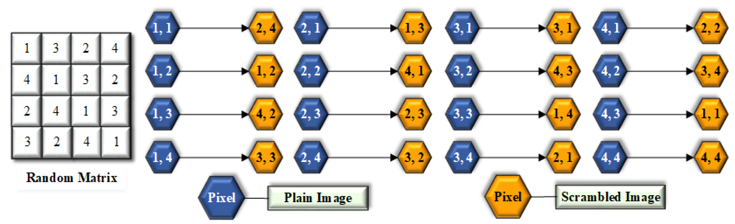
2.1. Scrambling Method

Scrambling is an easy and effective technique to lessen the correlation between the neighboring pixels. This paper introduced a one-to-one mapping for scrambling. Due to simultaneous changes of pixels in columns and rows, the proficiency of the algorithm enhanced enormously concerning time. The proposed algorithm has a one-to-one ratio between the pixels of scrambled image and the plain image, as displayed in Figure 1.
The pseudo-code of the scrambling method for Encryption process is described in Algorithm 1, while in the decryption process the same procedure is applied but using reverse shifting, as described in Algorithm 2.
Algorithm 1 Scrambling
  • Encryption Process:
  • Input: Generate S ( i , j ) matrix equal to the size of Plain image matrix P ( M , N ) .
  • Output: T ( m , n ) size Scrambled matrix.
  • Suppose for M = 4 and N = 4;
  • S Z ( M × N ) ; P Z ( M × N ) ; T Z ( M × N ) ;
  • A = Array sequence [ 3 , 2 , 1 , 4 ] ;
  • B = Array sequence [ 4 , 2 , 1 , 3 ] ;
  • I = A . i n d e x ( i ) for i in S o r t e d [ A ] ;
  • J = B . i n d e x ( j ) for j in S o r t e d [ B ] ;
  • P p i x e l s = 101 103 182 14 83 201 90 20 92 49 100 34 223 92 140 10
  • i m g = n p . z e r o s ( ( 4 , 4 ) ) ;
  • i m g [ 0 , : ] = [ 101 , 103 , 182 , 14 ] ;
  • i m g [ 1 , : ] = [ 83 , 201 , 90 , 20 ] ;
  • i m g [ 2 , : ] = [ 92 , 49 , 100 , 34 ] ;
  • i m g [ 3 , : ] = [ 223 , 92 , 140 , 10 ] ;
  • S = n p . z e r o s ( ( M , N ) ) ;
  • foriin range ( 0 , M ) ; do
  • for j in range ( 0 , N ) ; do
  •   m = [ ( j I ( i ) 1 ) m o d N ] + 1
  •    S [ i , m 1 ] = J [ j ]
  •    S = S + 1
  •   S
  • end for
  • end for
  • T = n p . z e r o s ( ( 4 , 4 ) )
  • forjin range ( 0 , N ) ; do
  • d a t a = [ ];
  • for i in range ( 0 , M ) ; do
  •   data.append.img [ I , S ( I , j ) 1 ]
  •   a = shift [ d a t a , ( N / 2 ) S ( 0 , j ) ]
  • end for
  • end for
  • forkin range 1 to N; do
  • T [ k , S [ k , j ] ] = a [ k ] ;
  • end for
  • S = 1 3 2 4 4 1 3 2 2 4 1 3 3 2 4 1 ; S c r . ( T ) = 140 103 83 100 34 223 90 101 92 20 14 92 201 182 49 10
Algorithm 2 Scrambling
  • Decryption Process:
  • Input: Random matrix S ( i , j ) and Cipher image matrix C ( M , N ) .
  • Output: Descrambled matrix P.
  • forjin range ( 0 , N ) ; do
  • d a t a = [ ];
  • for i in range ( 0 , M ) ; do
  •   data.append.img [ I , S ( I , j ) 1 ]
  •   a = shift [ d a t a , ( N / 2 ) S ( 0 , j ) ]
  • end for
  • end for
  • forkin range 1 to N; do
  • P [ k , S [ k , j ] ] a [ k ] ;
  • end for

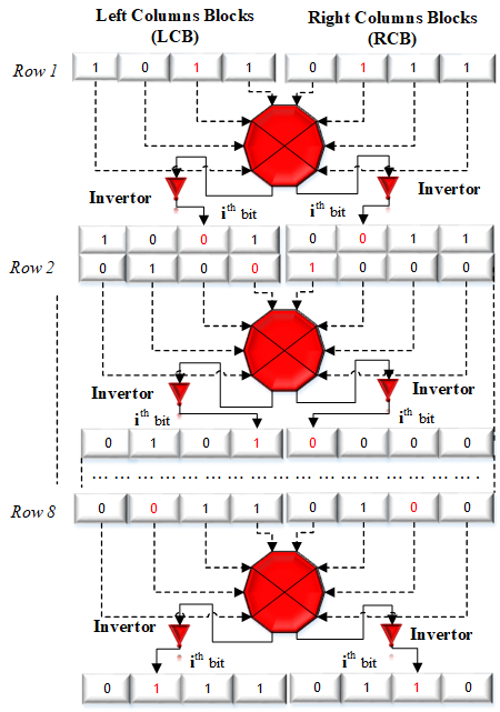
2.2. Novel Block Bit Inversion (BBI)

In this paper, we propose a novel blocked-based bit inversion technique to alter the pixel values. The Figure 2 is the graphical illustration of the proposed BBI structure for the image sub-matrix of the size M × N . Firstly, it divides the particular block matrix into two equal column blocks; labelled as Left bit Columns Blocks (LCB) and Right bit Columns Blocks (RCB). The purpose is to change the bits in every row and columns but in the opposite manner. It changes the particular bit 1 or 0 into opposite i.e., 0 if it is 1 or else 1 if it is 0. For each pixel, the change in value occurs (either addition or subtraction) depending upon either its get converted into 1 from 0 or get converted to 0 from 1. As each bit has a unique value, so because of bit inversion following change occurs in pixels based on the particular bit location.
M S B 8 t h b i t 2 8 1 = 2 7 = ± 128 ; 7 t h b i t 2 8 2 = 2 6 = ± 64
6 t h b i t 2 8 3 = 2 5 = ± 32 ; 5 t h b i t 2 8 4 = 2 4 = ± 16
4 t h b i t 2 8 5 = 2 3 = ± 8 ; 3 r d b i t 2 8 6 = 2 2 = ± 4
2 n d b i t 2 8 7 = 2 1 = ± 2 ; L S B 1 s t b i t 2 8 8 = 2 0 = ± 1
For example, we can see in Figure 2 that for each binary blocks the bit selection is in opposite direction means L C B b i t R C B b i t for left and right columns blocks. For the left columns block the selection of bit is from left to right L C B b i t R C B b i t and for the right columns block the selection of bit is from right to left L C B b i t R C B b i t . How its locate; is illustrated in Figure 3. Like in main diagram for the 1st row, 3rd bit is selected for the inversion in left columns block which is actually 6th while counting from right to left. In same passion, for the right columns block, 3rd bit is selected that is actually 6th when counting from left to right. So selection is the same for 3rd bit but direction is opposite as L e f t R i g h t . Thus, to select the particular bit in the novel BBI model, the formula efficiently locate the right and left block bits by proceeding only by the left to the right direction. The starting bit selection for each 8 × 8 blocks is based on the following formula.
L C B b i t n = [ ( n 2 × P m o d B + 1 ) + R i ] m o d B + 1
Here i = 1 , 2 , 3 , , 8 , where P is the pixel value of particular pixel, n is the block number multiplier to change the 1st bit for each block, B is the byte (8 bits), m o d is the mod function that returns the remainder between 0 to 7 because of B is one byte (8-bits), and R i is the particular row number range from 1 to 8.
For better understanding, Let suppose the decimal value of P for the 1st sub-matrix came 183, so the value of left columns block ( L C B b i t ) for the 1st row i = 1 or R i = 1 can be gotten as follows.
L C B b i t n = [ ( n 2 × P m o d B + 1 ) + R i ] m o d B + 1
L C B b i t 1 = [ ( 1 × 183 m o d 8 + 1 ) + 1 ] m o d 8 + 1
[ 7 + 1 + 1 ] m o d 8 + 1 = 1 + 1 = 2 n d b i t
Likewise, for the 2nd row of this 1st sub-block matrix, i = 2 or Ri = 2 the inverting bit will be;
L C B b i t 1 = [ ( 1 × 183 m o d 8 + 1 ) + 2 ] m o d 8 + 1
[ 7 + 1 + 2 ] m o d 8 + 1 = 2 + 1 = 3 r d b i t
Similarly, for the 3 r d , 4 t h , 5 t h to up to 8 t h rows for every L C B b i t n t h , desired inverting bit can be gotten through the formula. Alternatively, the formula of the bit selection for the right blocks is as follows.
R C B b i t n = [ B L C B b i t n ] m o d B + 1
As an example, in the above case after putting values.
R C B b i t 1 = [ 8 2 ] m o d B + 1 6 m o d 8 + 1 = 7 t h b i t
Similarly, for the 2nd row, the bit will be following.
R C B b i t 1 = [ 8 3 ] m o d B + 1 5 m o d 8 + 1 = 6 t h b i t
First of all, an initial configuration matrix of 8 × 8 is generated by the hash value of the key. Based on the above-mentioned formula of R C B b i t and L C B b i t , bit inversion is done over the initial configuration matrix ( I C M i t ) and later this updated initial configuration matrix ( I C M i t + 1 ) is XORed with the first plain matrix. The general equation of XORing the updated ( I C M i t + 1 ) with the plain image matrices is as follows.
S M n ( i , j ) t + 1 = S M 1 t I C M 0 t + 1 n = 1 S M n t I C M n 1 t + 1 n > 1
where n = 1 , 2 , 3 , , N ; where N is the entire number of sub-matrices of the red channel. While S M i t + 1 is the particular updated matrix, S M i t is the plain image sub-matrix of the red channel, and I C M i t + 1 is the updated initial configuration matrix. Similarly, for the 2nd sub-matrix bit inversion is performed over the updated initial configuration matrix of 1st block stage and then XORed with the second sub-matrix of the plain image as follows.
S M 2 t + 1 = S M 2 t I C M 1 t + 1
For the decryption phase, the reverse process to get back the plain image matrix is as follows.
S M n ( i , j ) t = S M 1 t + 1 I C M 0 t + 1 n = 1 S M n t + 1 I C M n 1 t + 1 n > 1
where n = 1 , 2 , 3 , , N and N is the total number of sub-matrices.

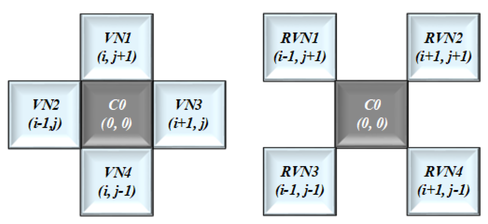
2.3. Two-Dimensional Cellular Automata

In this paper, a 2D-CA with VN and RVN structure was implemented as shown in Figure 4. Also, in cellular matrix form, every cell can have one of the two possible states that is either 1 or 0. In cellular representation every cell has its neighboring cells. The cell with VN neighbors or a radius equivalent to 1 can be represented in equation form as follow:
C v n t + 1 = δ ( C i , j + 1 t : C i 1 , j t : C i , j t : C i + 1 , j t : C i , j 1 t )
In this Equation (7), δ is the Boolean function or a state transition function that takes to the new state, where δ : C × ρ ( C ) . Like VN, the cell with Rotated VN neighbors can be represented as follow.
C r v n t + 1 = δ ( C i 1 , j + 1 t : C i + 1 , j + 1 t : C i , j t : C i 1 , j 1 t : C i + 1 , j 1 t )
So, to get the combined structure of VN and RVN, We merged these two equations as follows.
C M ( i , j ) t + 1 = δ ( C i 1 , j + 1 t : C i + 1 , j + 1 t : C i + 1 , j t : C i , j + 1 t : C i , j t : C i 1 , j + 1 : C i 1 , j 1 : C i + 1 , j 1 : C i + 1 , j + 1 )
We represent these 9 state variable with C N W : C N : C N E : C W : C 0 : C E : C S W : C S : C S E , as shown in Table 2. For the green channel as the bit depth or intensity is 28 so, we mapped the above mentioned 8 state variables with these eight bits as C N W ; C N ; C N E ; C W ; C E C S W ; C S ; C S E = [ 1 ; 1 ; 1 ; 1 ; 1 ; 1 ; 1 ; 1 ] , while excluding the central state variable C 0 ( 0 , 0 ) t represented as C 0 .
Finally, the confined rule structure is based on the following equation.
C M ( i , j ) t + 1 = ( C N W × C i 1 , j + 1 t ) ( C N × C i , j + 1 t ) ( C N E × C i + 1 , j + 1 t ) ( C E × C i 1 , j t ) ( C 3 × C i + 1 , j t ) ( C S W × C i 1 , j 1 ) ( C S × C i , j 1 ) ( C S E × C i + 1 , j 1 )
In this updated form of Equation (10); C N W , C N , C N E , C W , C E , C S W , C S , and C S E are the state variables that can have the values either 1 or 0. Therefore, the particular state variable will contribute in the XOR operation or state update process only if its respective bit will be equivalent to 1, otherwise it will not take part in the state update process.
Thus, the structural combination of above direction variables based on the binary value of decimal number is employed to elect which and whom cells/cell will take part in the state update process. Hence different binary representation means different confined rule equation for the matrix update process of each succeeding matrix. The general formula of the confined rules is given below.
C A C R = [ 2 ( I C M α t + I C M β t ) ] m o d F + 1 T = 1 ( T 1 ) α + ( T 1 ) β ] m o d F + 1 T > 1
In this formula α = count 0 s × 48 , β = count 1 s × 49 , I C M i t is the initial configuration matrix for the green channel that we got from the reserved hash (SHA-512) values for the green channel. F is the highest value of pixel that is 255. Whereas, T is the total number of blocks. For clear demonstration, let suppose we have the initial configuration matrix C 0 with a size 4 × 8 as given in Table 3.
From the ASCII table as the value of 1 is 49 and the value of 0 is 48, so the decimal value for the confined rule structure of the 1st sub-matrix can be found as follows.
C A C R = [ ( 12 × 48 ) + ( 20 × 49 ) ] m o d 255 + 1
C A C R = 26 + 1 = 27
Now converting this 27 into the binary form [00011011]2. As in this binary representation only 4 bits are 1, So only these 4 cells will participate in the XOR operation of 1st sub-matrix. To find those specific four cells we now put this binary value in Equation (10).
C M ( i , j ) t + 1 = ( 0 × C i 1 , j + 1 t ) ( 0 × C i , j + 1 t ) ( 0 × C i + 1 , j + 1 t ) ( 1 × C i 1 , j t ) ( 1 × C i + 1 , j t ) ( 0 × C i 1 , j 1 ) ( 1 × C i , j 1 ) ( 1 × C i + 1 , j 1 )
So Equation (12) will be simplified as follows.
C M ( i , j ) t + 1 = C i 1 , j t C i + 1 , j t C i , j 1 C i + 1 , j 1
This updated Equation (13) has four state variables that are C W = 1, C E = 1, C S = 1 and C S E = 1. So, only these four cells will contribute in the state update process of the 1st sub-matrix. From Table 2 we can see C i 1 , j t is actually C W , C i + 1 , j t is actually C E , C i , j 1 t is actually C S , while C i + 1 , j 1 t is actually C S E . Hence, by means of these confined rules structure, the processing power, computation time, efficiency and the security can be improved immensely.
The initial configuration matrix gets updated based on these confined rules mapping and then XORed with the particular plain image sub-matrix to acquire the updated matrix.
C k ( i , j ) t + 1 = C M ( i , j ) t + 1 C k ( i , j ) t
Here C k ( i , j ) t + 1 is the updated matrix, C M ( i , j ) t + 1 is the updated initial configuration based on confined rules, and C k ( i , j ) t is the plain image matrix. In decryption process the reverse equation to get back the original plain sub-matrix will be as follows.
C k ( i , j ) t = C M ( i , j ) t + 1 C k ( i , j ) t + 1

2.4. DNA Sequence

DNA molecule contain the genetic information that is used for the purpose of reproduction, functioning and growth of all living organism. Any DNA sequence comprised of four nucleic acid bases: Adenine (A), Cytosine (C), Guanine (G), and Thymine (T). These bases follow the principle of Watson–Crick, that is A and T are complementary, so are C and G same as in the binary system, 1 and 0 are complementary.
Likewise, the case of two-bits binary 11 and 00 are also complementary. Usually in DNA sequence every base is represented by the two-bits as 11, 10, 01 and 00 to represent these four bases T, G, C, and A respectively. There are basically 24 different kinds of DNA coding schemes. Nonetheless, out of those, only eight kinds fulfill the Watson–Crick complementary principle [51], which are given in Table 4. Please note that, like DNA encoding, the DNA decoding rules are just the inverse process of the DNA encoding rule.
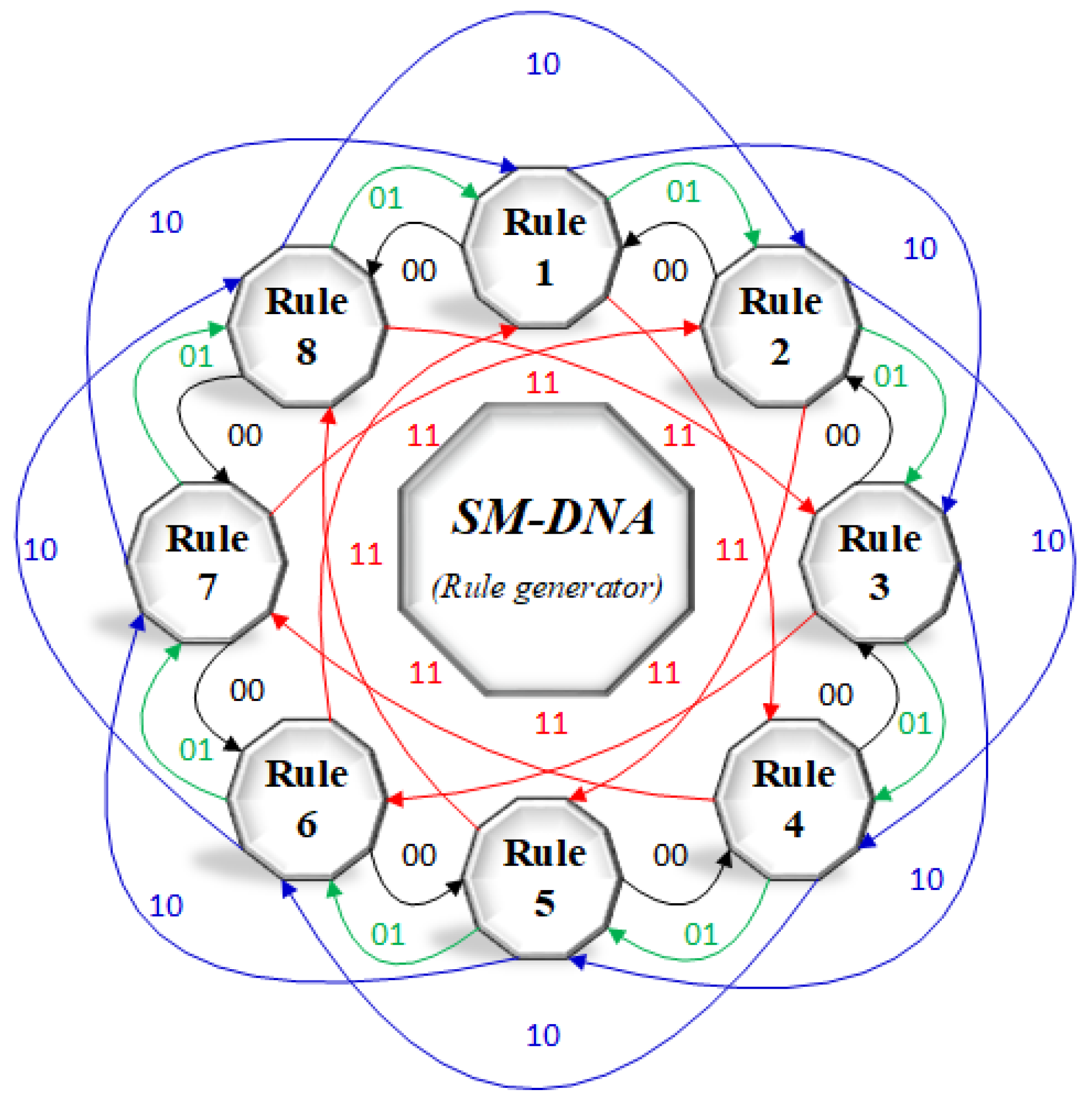
In this paper, we propose a new bidirectional mathematical model of DNA rule generator based on two bits of input as shown in Figure 5. The working principle of this model is based on Automaton state machine, so it is called the SM-DNA rule generator. SM-DNA generates random DNA rules faster than the chaotic serious-based rules selection method.
The pixel value of image matrix was converted into binary, then divided into sub-matrices form. We used i t h and j t h bits as an input. SM-DNA select random DNA rule for each block matrix. In our case, the first and last bit of every sub-block matrix was used as an input. The proposed SM-DNA model has eight states and each state represents one rule. Each state has 22 possible output states that take to next or previous state, so it means 84 = 4096 different rules combination, while rule transition from one to another depends solely on the following 4 combinations, either 11, 10, 01 or 00. For 00 it moves anti-clockwise direction and for 01, 10 and 11 it moves clockwise direction.
For ease of implementation binary matrix of the image was converted into 4 × 8 sub-matrices. SM-DNA allocated random DNA conversion rule to each sub-matrix very efficiently and quickly. For more clear understanding, working principle illustration is given in Figure 6 with a total of N binary sub-block matrices termed as B 1 , B 2 , B 3 , , B ( n 1 ) , B n . So the general formula of SM-DNA described as follows.
S M : D N A = [ ( N P 1 + N P 2 ) ] m o d B + 1 N = 1 ( N 1 ) k t h + ( N 1 ) n t h ] m o d B + 1 N 1
where kth and nth are the two particular bits of own choice to serve as an input for the rule selection, that is f i r s t b i t and l a s t b i t in our case. Suppose B M 1 s t is our first block matrix and also suppose the P1 and P2 value came out 109 and 207, respectively. So DNA starting rule for the 1st sub-block matrix can be gotten as follows.
S M : D N A 1 = ( 1 × 10⁹ + 1 × 207 ) m o d 8 + 1 = 5
So, Rule 5 will be the starting rule that will be used for binary to DNA conversion of 1st sub-block matrix.
B M 1 s t : : 10 11 01 01 00 11 00 01 00 10 10 01 10 11 11 11 R u l e 5 : : A G T T C G C T C A A T A G G G
For the 2nd sub-block matrix i t h = f i r s t b i t and j t h = l a s t b i t bit of 1st block matrix will be used that are 1,1. So, the Rule 8 is the conversion rule for 2nd sub-block matrix.
B M 2 n d : : 01 10 10 11 10 11 00 01 00 00 00 00 00 10 11 00 R u l e 8 : : G C C A C A T G T T T T T C A T
As input bits of the 2nd sub-block matrix are 0,0, So it went to state 7. Thus, Rule 7 will be the conversion rule for the 3rd sub-block matrix.
B M 3 r d : : 10 11 10 01 10 11 00 01 00 10 01 11 10 00 10 00 R u l e 7 : : G A G C G A T C T G C A G T G T
Similarly, all the sub-block matrices were converted into DNA sequences based on rules generated by SM-DNA as shown in Figure 6. Remember that for the N t h sub-block matrix the ( N 1 ) t h sub-block matrix will decide the rule. From security prospective as rule selection based on two bits inputs so it is very difficult to predict that out of 32-bits, which two-bits are working as an input. Thus its difficult to guess the rule selection without getting adequate information about the working principle of SM-DNA.

3. Proposed Encryption Method

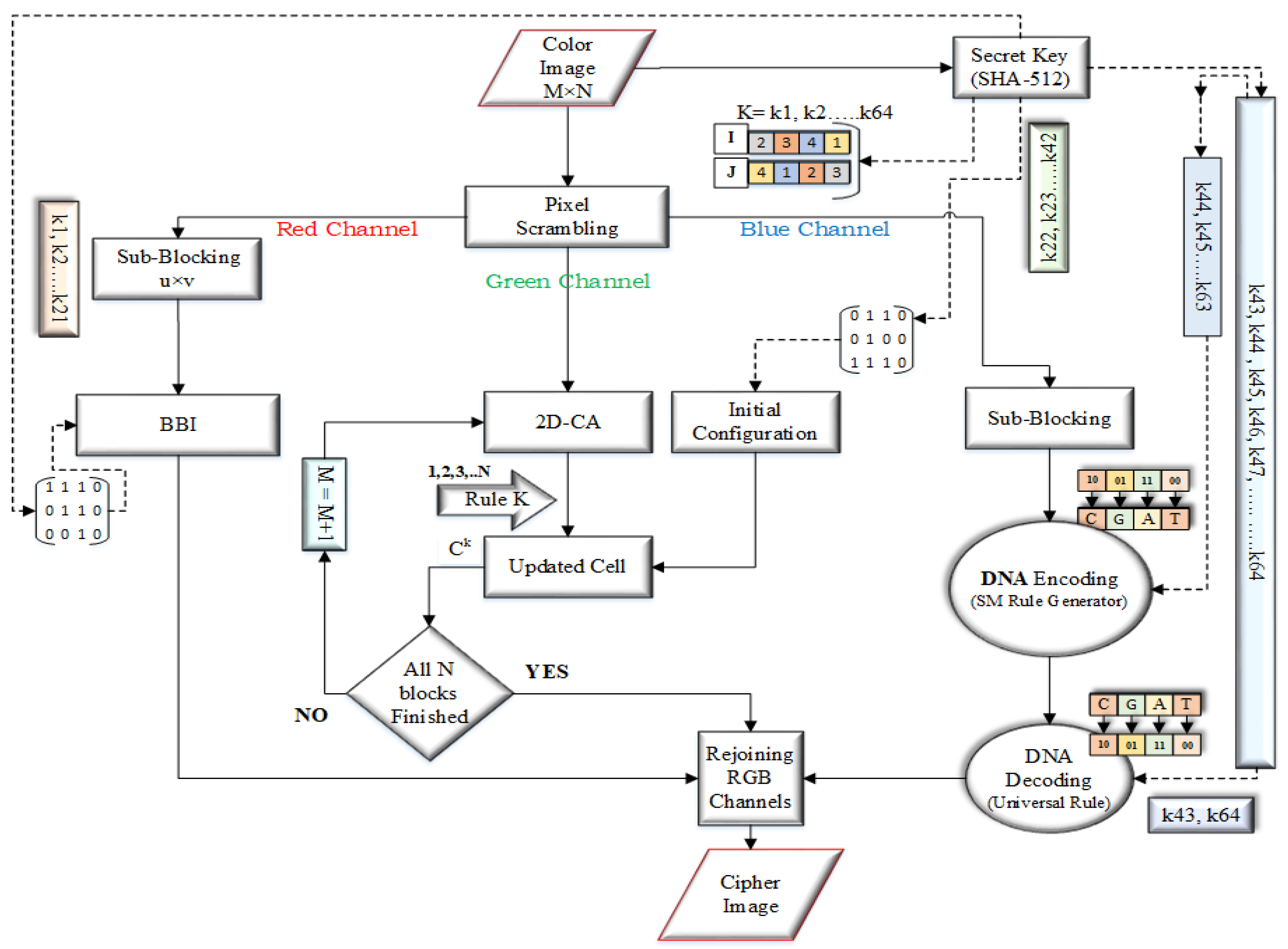
The general block diagram of the proposed image encryption method is shown in Figure 7. The proposed encryption method deal with the binary bit-planes of each channel. The detailed encryption steps are given below.
Step 1: Get the double hash-value of the image by using SHA-512. Hexadecimal forms of the key string will be gotten. Split the key string into three parts i.e., K 1 = 21 , K 2 = 21 and K 3 = 22 hexadecimal pairs to use in the formulas and initial configuration matrices of red, green and blue channels as follows.
K r e d = k 1 , k 2 , k 3 , k 4 , , k 20 , k 21
K g r e e n = k 22 , k 23 , k 24 , k 25 , , k 41 , k 42
K b l u e = k 43 , k 44 , k 45 , k 46 , , k 63 , k 64
Step 2: Take the color image ( M , N , 3 ) , where M and N denote the rows and columns of the image, respectively. Scramble as described in the scrambling portion, while the hexadecimal form of a key was used as a seed to generate array sequence by L S S P R N G . For the two rounds of sequences, the seed values are set through the following equations.
x 0 = ( k 1 k 2 k 3 k 4 ) + + ( k 13 k 14 k 15 k 16 ) 256
y 0 = ( k 17 k 18 k 19 k 20 ) + + ( k 29 k 30 k 31 k 32 ) 256
z 0 = ( k 33 k 34 k 35 k 36 ) + + ( k 45 k 46 k 47 k 48 ) 256
The integer values for two round from the n b i t s of the stream gotten by the following formula.
i n t e g e r = i = 1 n b i × 2 i 1
For the two rounds of array sequence the initial state can be set by the following way.
X 0 i = [ i n t e g e r × y 0 × ( x 0 + z 0 ) ] m o d 1 r i = [ i n t e g e r × x 0 × ( y 0 + z 0 ) ] m o d 4
where, i = ( 1 , 2 ) termed as rounds and it will generate two initial values X 0 1 , r 1 and X 0 2 , r 2 respectively.
Step 3: Split the scrambled color image T ( M , N , 3 ) S c r . into respective three channels R, G and B channels and we can get the three components, T R S c r . , T G S c r . and T B S c r . as given below.
T R S c r . = T r 1 , T r 2 , T r 3 , , T r M N
T G S c r . = T g 1 , T g 2 , T g 3 , , T g M N
T B S c r . = T b 1 , T b 2 , T b 3 , , T b M N
Here T r i , T g i and T b i are the i t h pixel values of the red, green and blue channels respectively, whereas T r i ; T g i ; T b i [ 0 , 255 ] . Transformed the pixel values of each channel into the binary windows as given below.
T R ( M , N ) = R w 1 , R w 2 , R w 3 , , R w 8
T G ( M , N ) = G w 1 , G w 2 , G w 3 , , G w 8
T B ( M , N ) = B w 1 , B w 2 , B w 3 , , B w 8
Now split the window matrix into m × n size sub-blocks, where u × m = M and v × n = N.
Step 4: Take the 1 s t block of T R ( M , N ) with a size 8 × 8 and split it into two equal columns block e.g., 8 × 4 and 8 × 4 ; termed as LCB and RCB. By using formula get the starting bit for the 1st block-matrix and apply block bit inversion as described in Section 2.2.
Step 5: Take the green channel T G ( M , N ) and apply the Cellular Automata as described in Section 2.3.
Step 6: Take the blue channel T B ( M , N ) of size H × W divide it into the u × v size sub-blocks matrices as given below. While u × H = M and v × W = N , and apply DNA conversion as described in Section 2.4.
T B ( M , N ) b i = B M 1 b i , B M 2 b i , B M 3 b i , , B M ( n 1 ) t h b i , B M n t h b i
With SM-DNA convert every binary block matrix into DNA matrix based on allocated rule of SM-DNA as follows.
B M 1 b i B M 1 D N A , B M 2 b i B M 2 D N A , B M 3 b i B M 3 D N A
, , B M ( n 1 ) b i B M ( n 1 ) D N A , B M n t h b i B M n t h D N A
Join all these DNA sub-block matrices into a single matrix as described below.
B M 1 D N A , B M 2 D N A , B M 3 D N A , , B M n t h D N A = T B ( M , N ) D N A
Get the universal D N A b i n a r y rule through following formula.
D N A U R = [ P 1 + P 2 ] m o d 8 + 1
Convert the whole DNA sequence matrix back into binary form through this universal rule.
Step 7: Add the random matrix of the scrambling part to the pixel values of each channel as described below.
C i p h e r R G B C ( i , j ) r e d = [ E ( i , j ) r e d + R ( i , j ) ] m o d 256 C ( i , j ) g r e e n = [ E ( i , j ) g r e e n + R ( i , j ) ] m o d 256 C ( i , j ) b l u e = [ E ( i , j ) b l u e + R ( i , j ) ] m o d 256
where C ( i , j ) denotes cipher value of particular pixel, E ( i , j ) denotes encrypted value of the pixel, R ( i , i ) denotes the Random matrix, i = 1 , 2 , M , and j = 1 , 2 , , N .
Step 8: Rejoin all the channels to get the cipher image.
C i p h e r ( M , N , 3 ) = C ( i , j ) r e d ; C ( i , j ) g r e e n ; C ( i , j ) b l u e

4. Experimental Results and Discussion

This section included the performance and simulation results along with the comparison of results with earlier proposed image encryption schemes. The experimental results were manipulated in Python 3.6.5 (Jupyter Notebook Environment) installed over a personal Laptop, CPU Intel Core I5 with 4GB memory and operating system Window 10.
The test image baboon, its cipher image and the decrypyted image are shown in Figure 8. The experimental parameters are given in Table 5. Whereas all the test images that we used for experiments are shown at the end of paper in Figure 9.

5. Security Analysis and Test

5.1. Security Keyspace

The keyspace represents the entire number of likely combinations of the security key. The most common attack is the Brute-force attack in which an attacker endeavors to predict the accurate security key by overly searching the keyspace of the encryption algorithm. Thus, in order to withstand against the Brute-force attack, an adequately huge keyspace is one of the main factor that can guarantee more security [52].
For resisting the best attack, secure hash algorithm (SHA-512) uses a keyspace of 2256. The comparison of keyspace and approach along with testing parameters of the proposed algorithm is given in Table 6.
Moreover, the SM-DNA possible rules combination 84 can also be taken as keyspace. Except for the fact that the hash keys for generating initial configuration matrices for each channel and in their particular rule generating formulas are 222, 222, 221, and 25 respectively. So, the overall keyspace of the proposed algorithm is 2 256 × 2 21 × 2 22 × 2 22 × 2 5 × 8 4 which is very large as compared to 2128. To calculate the computational load, let’s the fastest computer computes 2 80 computations in 1 second and 2 80 × 365 (days) × 24 (h) × 60 (min) × 60 (s) [57]. So, to compute 8 4 × 2 > 310 computations, a total of following years required.
8 4 × 2 > 310 2 80 × 365 × 24 × 60 × 60 2 . 68 × 10 65 y e a r s
This huge computation load is sufficient enough to break the crypto-system. The computational load also proved that the 3C3R can effectively withstand against the brute-force attacks.

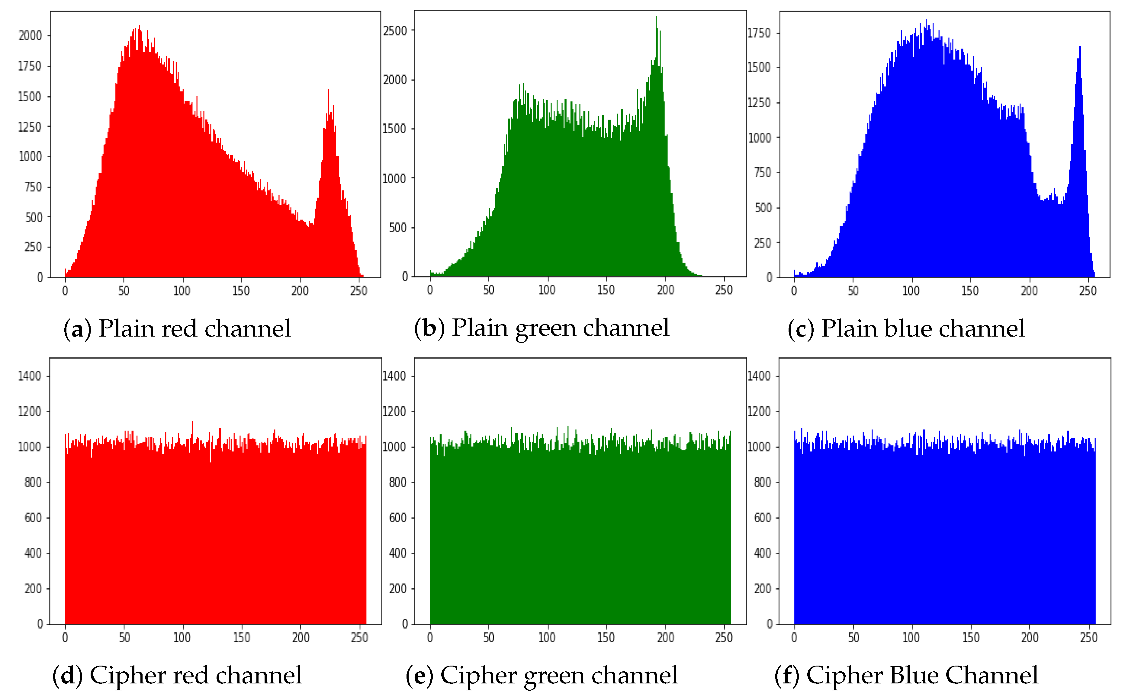
5.2. Histogram Analysis

The histogram of an image demonstrate the distribution of the pixel values. An intruders usually recover the meaningful information from the fluctuating histogram of the encrypted image. So, in order to prevent an intruder from recovering such information, it is important that the histogram of the cipher-image should have no statistical resemblance to the plain image and also should have uniform distribution. The histograms of the ciphered images of all the test images are shown in Figure 10. While Figure 11 shows the histogram of RGB channels of the plain image and its corresponding cipher image. The histogram of the each RGB channel of the cipher image is almost uniform. Moreover, by computing the variance of histogram, we evaluated the uniformity of our ciphered images. The lesser the variance means the higher is the uniformity of the encrypted images [58,59,60,61].
v a r ( I ) = 1 k 2 i = 1 k j = 1 k 1 2 ( I i I j ) 2
Table 7 listed the histogram variances of the plain images (R,G,B) and encrypted images along with a comparison with the other methods. From the table, we can see that in most of the test images the histogram variance of the proposed algorithm is less as than from Ref. [62] and Ref. [49]. This proved that the 3C3R has better security in comparison to those algorithms.

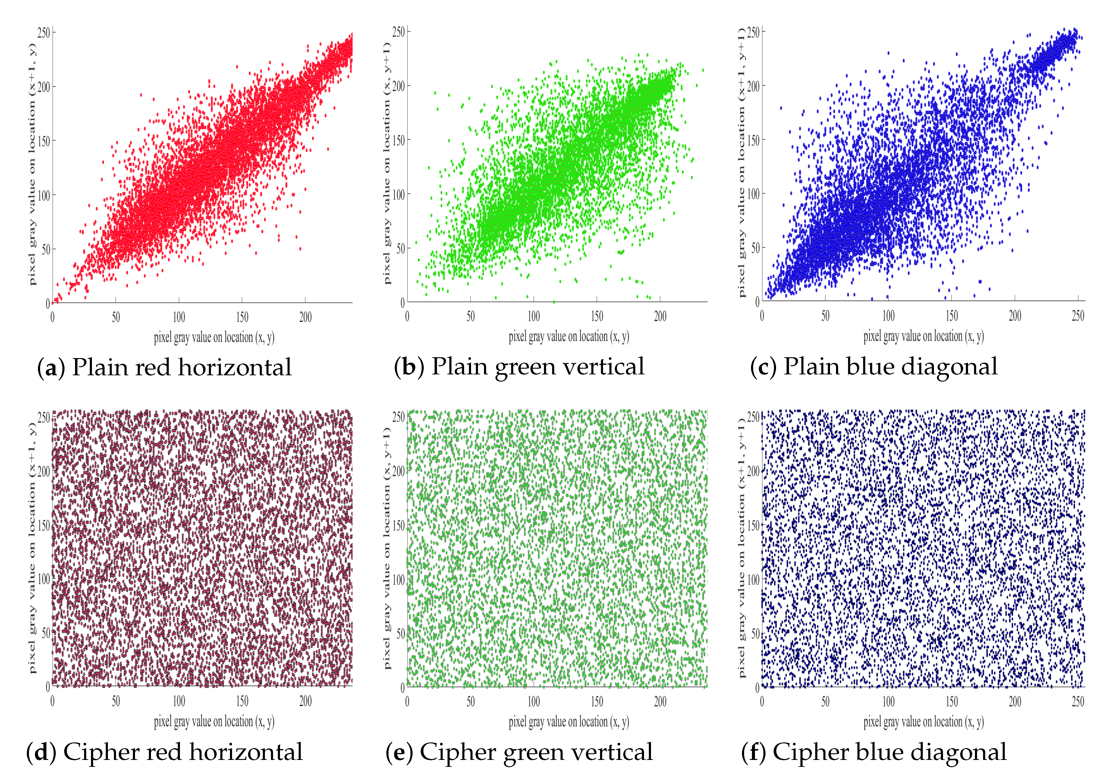
5.3. Pixel Correlation Analysis

Pixel correlation analysis is another test used to find the relationship of neighboring pixels in the plain image and the ciphered image. A good encryption algorithm aims to minimize the relationship among the neighboring pixels with regards to prevent the leakage of actual information.
The correlation coefficient Cr(x,y) between the two neighboring pixels can be calculated by the following formulas.
E ( w ) = 1 P i = 1 P w i
D ( w ) = 1 P i = 1 P ( w i E ( w ) ) 2
C o v a r i a n c e ( w , z ) = 1 P i = 1 P ( w i E ( w ) ) ( z i E ( z ) )
C r ( w , z ) = C o v a r i a n c e ( w , z ) D ( w ) × D ( z )
In above equations (w, z) is the gray values of neighboring pixels, Covariance(w,z) is the covariance, P is the total number of pixels selected from the image, while E(w) is the mean and D(w) is the variance. Figure 12 displays the pixels of the plain image and ciphered image of the proposed algorithm in horizontal (H), vertical (V) and diagonal (D) distribution. In Table 8 and Table 9 the pixel correlation comparison was done with some previous algorithms. Table 8 shows a comparison of 8K pairs of neighboring pixels that are randomly selected from the plain image and the ciphered image in the H, V, and D directions to perform pixel correlation analysis. Whereas, Table 9 shows a correlation comparison of 1K random pixels of the Lena image. Whereas, Table 10 listed the pixel correlation values of the different test images.
We casually selected the pixel pairs in the horizontal, vertical and diagonal axes, respectively. From Table 9 it is obvious that in term of overall correlation, proposed 3C3R and Ref. [63] are performing well, while in term of diagonal values our algorithm, Refs. [63,64,65] are giving satisfactory values. While the overall and in terms of UACI and NPCR, the proposed 3C3R outperformed.
Similarly, for 8K random pixels the Refs. [55,58,66,68,70] are giving good results but the proposed 3C3R is also performing well in regards to vertical and diagonal direction.

5.4. Key Sensitivity Analysis

Because of the enhanced computational power, the current era’s encryption algorithms should not have key length less than 100 bits or ( 2 100 ). Such key length can withstand against the exhaustive key search attack (brute force attack). The keyspace of the proposed encryption method is 2 ( > 312 ) , which has high ability to resist the brute-force attack. Except for the fact that the key should also be extremely sensitive to the bit change. If the secret key will not be subtle enough, then a slight change in the actual secret keys can also properly recover the original image. Also, the secret key may perverted and as a result the actual keyspace may less than the theoretical one [60,61,78].
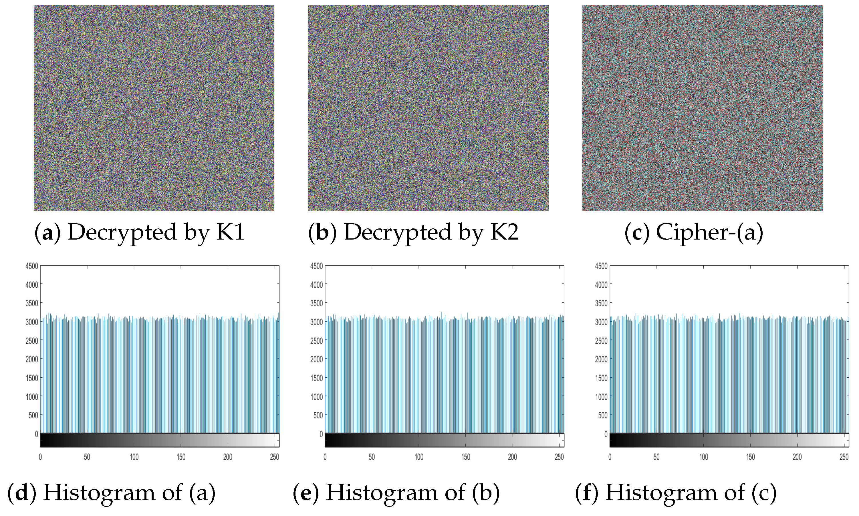
So, to check the sensitivity of the proposed algorithm towards the key, experiment has performed by changing one bit in the key with respect to the actual key as shown below.
Keyo = “40 CD 74 4F 66 82 BD 0A CF 73 57 9A 5D C3 53 DB 3A 29 5D 3A 2D 87 03 56 6C 8A CF 9B E8 AA 68 8E 87 62 1E 8F 5F 3D 07 37 63 C4 6E 93 FF 7B 1A 2B 04 76 C3 BB 84 08 F2 A2 E8 AF AB 48 08 7B B9 C4”.
Key1 = “40 CD 74 4F 66 82 BD 0A CF 73 57 9A 5D C3 53 DB 3A 29 5D 3A 2D 87 03 56 6C 8A CF 9B E8 AA 68 8E 87 62 1E 8F 5F 3D 07 37 63 C4 6E 93 FF 7B 1A 2B 04 76 C3 BB 84 08 F2 A2 E8 AF AB 48 08 7B B9 C5”.
Key2 = “50 CD 74 4F 66 82 BD 0A CF 73 57 9A 5D C3 53 DB 3A 29 5D 3A 2D 87 03 56 6C 8A CF 9B E8 AA 68 8E 87 62 1E 8F 5F 3D 07 37 63 C4 6E 93 FF 7B 1A 2B 04 76 C3 BB 84 08 F2 A2 E8 AF AB 48 08 7B B9 C4”.
Keyo is the actual key while Key1, Key2 are the one-bit changed keys from LSB (Right) and MSB (left) bit respectively. Figure 13a,b show the decrypted image by Key1 and Key2 respectively. Both Key1 and Key2 are one bit different from the actual key but the decrypted image is still like noise giving no useful information. The Figure 13c is the subtracted image of the actual cipher and the decrypted image of Key1. The histogram of particular three resultant images is given in Figure 13d–f respectively. The subsequent uniform histograms proved that the proposed 3C3R is very sensitive to key change even one-bit change leads towards totally different cipher image.

5.5. Differential Attack

Normally, hackers; to extract useful information create little modification in the plain image and then by using the encryption methodology they encrypt the identical images afore and afterwards these slight changes. Through this method, they attempt to find out the association among the plain images and the cipher images. Thus, we employed the number of pixel change rate (NPCR) and unified average changing intensity (UACI) to measure the robustness of the proposed algorithm against such attacks. The NPCR and UACI can be calculated by the following way.
N P C R U 1 , U 2 = [ r , c I ( r , c ) H × M ] × 100
U A C I U 1 , U 2 = 1 H × M [ r , c | U 1 ( r , c ) U 2 ( r , c ) | 2 8 1 ] × 100
Here U1, U2 are two different ciphered images before and after one pixel of the plain image is changed, while H × M is the height and width of the test image. Whereas, I(r, c) can be defined as
I ( r , c ) = 0 U 1 ( r , c ) U 2 ( r , c ) 1 o t h e r w i s e
In the above equation, I depict the difference between U1 and U2.
Table 11 listed the NPCR and the UACI values of different test images along the comparison with some earlier algorithms. From the table values, we can see the test results of the Lena and pepper images of our 3C3R giving NPCR99.97 and UACI33.46. NPCR is high from Refs. [28,58,59,79,80], while it is comparable to [81]. Similarly, UACI is also comparable with the Refs. [59,79,81]. Thus the proposed 3C3R has satisfactory security values.

5.6. Known and Chosen Plain Text Analysis

Most commonly, four kind of cryptanalsis attacks can be performed to crack the image encryption algorithms that are chosen-cipher-text attack, chosen-plaintext attack, cipher-text only attack, and known-plaintext attack [82]. Some famous image encryption algorithms given in Table 1 have already been broken with these attacks.
The cryptanalysis model, where the attackers choose plaintext to obtain the corresponding cipher-text is called chosen-plain text attack. By examining the plaintext and the corresponding cipher-text, they try to presume some hidden useful information. Finally, by using that information they try to recover the original images [85,86].
The chosen-plaintext attack is the most powerful, and if the encryption may resist this attack, it has adequate security level to withstand the other three attacks. The proposed algorithm 3C3R has satisfactory security level against known and chosen plaintext attacks.
We can see the cumulative entropy(R,G,B) value is 8.00. In Table 15 comparison of the entropy values was also given, the value is higher from Refs. [82,87,88,
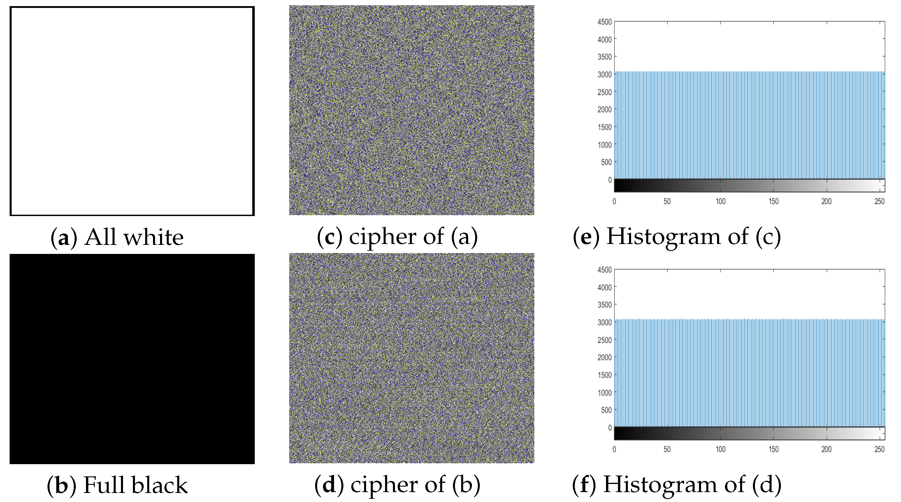
89]. The proposed algorithms give the ideal all channels entropy values for all white, full black image and is given in Table 16. The proof of ideal entropy value is visible in the histogram of the ciphered image generated by our 3C3R of all white and full black, and was given in Figure 14. The histogram of all white, full black and Playboy image is almost entirely flat. Furthermore, we created two special color images SPimage1 and SPimage2 respectively of size P × Q × 3 . SPimage1 is the color image with all pixels’ values 0 except one pixel located at (252, 252) in R channel is 1. Similarly SPimage2 is the color image with all pixels’ values 1 except one pixel located at (252, 252) in R channel is 0. We made plaintext sensitivity analysis and the results are given in Table 12. The average values of NPCR and UACI are closed to the theoretical value. Thus on the bases of this test we can say that 3C3R is robust against such attacks and can keep the image more secure.

5.7. Robustness against Occlusion Attack

In image processing, PSNR and MSE are the most widely used parameters to test the encryption quality. The PSNR and MSE values can be calculated as follows.
P S N R = 10 × l o g 10 ( 255 × 255 × 3 M S E R + M S E G + M S E B ) ( d B )
M S E = 1 M N r M c N I p ( r , c ) I c ( r , c ) 2
where M S E R , G , B is the mean square error of red, blue and green channel, between the cipher image I c ( r , c ) and original image I p ( r , c ) , while M and N is the height and width of the image respectively.
Another way is quality checking at the receiver side, such as after passing through a noisy medium cipher, an image may get blurred or lose some data. Therefore, a trustworthy encryption scheme should be able to recuperate the original image without losing too much substantial information. Figure 15a–f shows the different test images with different cropped portion. While Figure 15g–l are the retrieved images, we can see the retrieved images are easily recognizable and carry good information even after clipping 1/2. While the less clipping gave a much better result. Table 13 listed the PSNR and MSE comparison with [29] of test image Lena with different proportion of cropping. The values show that our algorithm performs better when increased the clipping portion while values are comparable for the less clipping.
Measuring the difference between the cipher image and original image is another way to evaluate the quality of the color images. So, for this purpose the PSNR can be viewed as a security evaluation parameter. The encryption effect is consider better if the value of PSNR is lower. Table 14 listed the PSNR value between p l a i n d e c r y p t e d and p l a i n c i p h e r e d images. The comparison was also made with some well-known algorithms and values are listed in the particular table. We can see from the table that the PSNR value for the different test images is P S N R 8.10 that is lower than Refs. [15,23,46,90,91] except the test image baboon in which Ref. [15] gave the lowest PSNR value between plain image and ciphered image. Thus, based on the PSNR value test, we can say that our 3C3R performs very well and can guaranty more security in comparison to other algorithms.

5.8. Local and Shannon Information Entropy

The information entropy ( I E ) defines the degree of disorder or chaos in an encryption system through the gray value probability. IE for the image can be defined as follow:
Let an information source be a τ , then I E can be computed as follows.
H ( τ ) = i = 0 2 n 1 ρ ( τ i ) l o g 10 1 ρ ( τ i )
Here ρ ( τ i ) depicts the probability of the symbol τ i . The ideal IE value for the image with gray intensity level of 28 is 8 [93]. So, it means the closer the IE value, the more is the randomness of an image, and as a result less information will be revealed by the particular encryption scheme. Table 15 and Table 16 enlisted the entropy value of some famous test images and their comparison with some earlier encryption algorithms. The table values are the evidence of IE7.996, that is close enough to the ideal value 8.0. While for Playboy, full white and Full black 3C3R achieved the ideal value IE = 8.00. IE values of all the test images are higher than Refs. [82,87,88,89].
In [94] a new image uncertainty test introduced by means of Shannon entropy over the native image-blocks. The (k, TP) Shannon entropy measure concerning local image blocks can be calculated by the following method:
Step 1: Select the non-overlapping image blocks randomly i.e., B 1 , B 2 , B 3 , , B k with TP Pixels within the ciphered or test image I with intensity scales L.
Step 2: Compute Shannon entropy for all i ( 1 , 2 , 3 , , k ) by using Equation (44).
Step 3: Calculate the Shannon entropy sample mean over these k image blocks B 1 , B 2 , B 3 , , B k by the following equation.
H ¯ ( k , T P ) ( B ) = i = 1 k H ( B i ) k
The local Shannon entropy value was calculated for the ciphered images. Firstly, non-overlapping image blocks with k = 32 and TP = 1936 pixels are randomly selected from the ciphered images. As the experiential value of local Shannon entropy must fall within the confidence interval i.e., [7.9019, 7.9030], concerning the α -level sureness equal to the 0.05. Table 16 listed the Shannon entropy and global entropy values and also the comparison of Shannon entropy with Ref. [95]. The Shannon entropy value of the ciphered image of the proposed 3C3R fully falls within the desired range. Thus, based on the ideal IE values, we can say the ciphered image generated by the proposed 3C3R carries more haphazardness and as a result, assures more security.

5.9. Gray Value Degree (GVD) Analysis

The gray difference degree or GVD is another statistical test of haphazardness that can be found by comparing the plain image and the ciphered image. The ideal value is 1, so closer the value the better is the security. GVD can be computed by the following Equation;
G D ( r , c ) = [ G ( r , c ) G ( r , c ) ]
whereas G ( r , c ) symbolizes the gray score at position ( r , c ) and ( r , c ) is as given below.
( r , c ) = ( r 1 , c ) ( r + 1 , c ) ( r , c 1 ) ( r , c + 1 )
The average neighborhood gray difference of the whole image can be computed as follows.
A V e r a g e [ G D ( r , c ) ] = r = 2 M 1 c = 2 N 1 G D ( r , c ) ) ( M 2 ) ( N 2 )
A V e r a g e G V D = A V [ G D ( r , c ) ] A V [ G D ( r , c ) ] A V [ G D ( r , c ) ] + A V [ G D ( r , c ) ]
In these equations, A N and A N , denotes the average neighborhood gray value; but the former represents after encrypting and the later represents before encryption. The final GVD value termed as gray value degree and it will be 1 if the two images are completely different or else it will be 0, if the two images are same. The GVD score of the plain and encrypted images of USC-SIPI database are shown in Table 17. The GVD score for most of the test images is GVD ≥ 0.907 for each R, G and B channel which shows that the plain and encrypted images are entirely different. The listed results also show that 3C3R ensures more security for images as compared to Refs. [29,69,97] except for the image 4.1.04 in which Ref. [29] has the higher value as compared to 3C3R.

5.10. Performance Comparison

Performance and encryption time are an important characteristic of any image encryption algorithm. Like in the Chaos-based encryption schemes, number of permutation and diffusion rounds have a direct impact over the encryption time. Similarly for color image rule processing scheme over the RGB channels has a direct relation with the encryption time. Because of the parallel processing characteristics of cellular automata and DNA sequence the proposed 3C3R takes less encryption time as compared to chaos-based schemes. Table 18 enlisted the time comparison of our 3C3R with the Refs. [79,81,98,99] that possess a satisfactory security level. The least encryption and decryption time was taken by the proposed 3C3R shows that our algorithm gives satisfactory results with minimum times. Except that Table 19 listed the comparison with the recently introduced algorithms. The table values in bold fonts clearly concludes that our 3C3R overall performing much better than Refs. [56,62,76,91]. Hence, our 3C3R assures better image security.

6. Conclusions and Future Work

To conquer the issue of low sensitivity to the secret key or low security against known plain or cipher-text attacks, this paper introduced a 3C3R robust image encryption algorithm with adequate security level against well known attacks. Fully uniform histogram and ideal cumulative entropy 8.00 for some images are the proof of robustness and better security of an image by 3C3R. Unlike most encryption methodologies in which the same encryption method or rules structure followed for all channels, this paper introduced a novel encryption method comprising different encryption strategy for each channels. Block bit inversion (binary) for the red channel, VN and RVN (cellular) structure-based pixel alteration for the green channel, and state machine-based SM-DNA rule allocation for the blue channel. Experimental results proved that our 3C3R algorithm is highly subtle to the secret key along with better security. The proposed 3C3R can keep different types of images safe and secure from attackers. 3C3R outperforms state of the art algorithms in terms of encryption performance and image security. The experimental results also proved that the 3C3R is robust against well-known attacks such as brute-force attacks, occlusion attacks, chosen/known plaintext attacks, and differential attacks. Therefore, we can say that 3C3R is the algorithm of the current era requirement and hence it has potential applications in multimedia communication.

Author Contributions

S.K. conceived, designed as well as performed all the experiments including writing the manuscript; L.H. supervised the research and delivered funding acquisition; G.M. designed the methodology; B.G. worked over editing and visualization; H.U. performed formal analysis.

Funding

This research was funded by the National Natural Science Foundation of China grant number “N0:61272033, 61572222”.

Conflicts of Interest

The authors declare no conflict of interest. The founding sponsors had no role in the data collection, data analyses, or interpretation of results; as well as in the writing of the manuscript, and in the decision of publishing the results.

References

  1. Wong, K.; Kwok, B.; Law, W. A fast image encryption scheme based on chaotic standard map. Phys. Lett. A 2008, 372, 2645–2652. [Google Scholar] [CrossRef] [Green Version]
  2. Gehani, A.; LaBean, T.H.; Reif, J.H. DNA-based cryptography. In Aspects of Molecular Computing; Springer: Berlin/Heidelberg, Germany, 2003; Volume 54, pp. 233–249. [Google Scholar]
  3. Lian, S.G. Multimedia Content Encryption: Techniques and Applications; Auerbach Publication Taylor & Francis Group: Boca Raton, FL, USA, 2008; ISBN 1420065270. [Google Scholar]
  4. Wang, Y.; Wong, K.; Liao, X.; Xiang, T.; Chen, G. A chaos-based image encryption algorithm with variable control parameters. Chaos Solitons Fract. 2009, 41, 1773–1783. [Google Scholar] [CrossRef]
  5. Guan, Z.H.; Huang, F.; Guan, W. Chaos-based image encryption algorithm. Phys. Lett. A 2005, 346, 153–157. [Google Scholar] [CrossRef]
  6. Yavuz, E.; Yazici, R.; Kasapbasi, M.C.; Yamac, C. A chaos-based image encryption algorithm with simple logical functions. Comput. Electr. Eng. 2016, 54, 471–483. [Google Scholar] [CrossRef]
  7. Dou, Y.; Liu, X.; Fan, H.; Li, M. Cryptanalysis of a DNA and chaos based image encryption algorithm. Optik 2017, 145, 456–464. [Google Scholar] [CrossRef]
  8. Chen, J.; Zhang, Y.; Qi, L.; Fu, C.; Xu, L. Exploiting chaos-based compressed sensing and cryptographic algorithm for image encryption and compression. Opt. Laser Technol. 2018, 99, 238–248. [Google Scholar] [CrossRef]
  9. Jeng, F.G.; Huang, W.L.; Chen, T.H. Cryptanalysis and improvement of two hyper chaos based image encryption schemes. Signal Process. 2015, 34, 45–51. [Google Scholar] [CrossRef]
  10. Qin, Y.; Wang, Z.; Wang, H.; Gong, Q. Binary image encryption in a joint transform correlator scheme by aid of run length encoding and QR code. Opt. Laser Technol. 2018, 103, 93–98. [Google Scholar] [CrossRef]
  11. Kumar, R.; Bhaduri, B. Optical image encryption using Kronecker product and hybrid phase masks. Opt. Laser Technol. 2017, 95, 51–55. [Google Scholar] [CrossRef]
  12. Chen, H.; Tanougast, C.; Liu, Z.; Blondel, W.; Hao, B. Optical hyperspectral image encryption based on improved Chirikov mapping and gyrator transform. Opt. Lasers Eng. 2018, 107, 62–70. [Google Scholar] [CrossRef]
  13. Li, X.; Meng, X.; Yang, X.; Wang, Y.; Yin, Y.; Peng, X.; He, W.; Dong, G.; Chen, H. Multiple-image encryption via lifting wavelet transform and XOR operation based on compressive ghost imaging scheme. Opt. Lasers Eng. 2018, 102, 106–111. [Google Scholar] [CrossRef]
  14. Chai, X.; Gan, Z.; Yang, K.; Chen, Y.; Liu, X. An image encryption algorithm based on the memristive hyper-chaotic system, cellular automata and DNA sequence operations. Signal Process. 2017, 52, 6–19. [Google Scholar]
  15. Wu, X.; Wang, K.; Wang, X.; Kan, H.; Kurths, J. Color image DNA encryption using NCA map based CML and one time keys. Signal Process. 2018, 148, 272–287. [Google Scholar] [CrossRef]
  16. Talarposhti, K.M.; Jamei, M.K. A secure image encryption method based on dynamic harmony search (DHS) combined with chaotic map. Opt. Lasers Eng. 2016, 81, 21–34. [Google Scholar] [CrossRef]
  17. Lian, S. A block cipher based on chaotic neural networks. Neurocomputing 2009, 72, 1296–1301. [Google Scholar] [CrossRef]
  18. Zhang, X.; Chen, W. A new chaotic algorithm for image encryption. In Proceedings of the 2008 International Conference on Audio, Language and Image Processing, Shanghai, China, 7–9 July 2008; pp. 889–892. [Google Scholar] [CrossRef]
  19. Xue, X.L.; Zhang, Q. An image fusion encryption algorithm based on DNA sequence and multi-chaotic maps. J. Comput. Theor. Nanosci. 2010, 7, 397–403. [Google Scholar] [CrossRef]
  20. Zhou, Y.; Bao, L.; Chen, C.L.P. A new 1D chaotic system for image encryption. Signal Process. 2014, 97, 172–182. [Google Scholar] [CrossRef]
  21. Hua, Z.; Zhou, Y.; Pun, C.M. Image encryption using 2D Logistic-Sine chaotic map. In Proceedings of the 2014 IEEE International Conference on Systems, Man, and Cybernetics (SMC), San Diego, CA, USA, 5–8 October 2014; pp. 3229–3234. [Google Scholar]
  22. Zamani, S.; Javanmard, M.; Jafarzadeh, N. A novel image encryption scheme based on hyper chaotic systems and fuzzy cellular automata. In Proceedings of the 2014 22nd Iranian Conference on Electrical Engineering (ICEE), Tehran, Iran, 20–22 May 2014; pp. 1136–1141. [Google Scholar]
  23. Norouzi, B.; Mirzakuchaki, S. A fast color image encryption algorithm based on hyper-chaotic systems. Nonlinear Dyn. 2014, 78, 995–1015. [Google Scholar] [CrossRef]
  24. Khan, S.; Han, L.; Lu, H.; Butt, K.K.; Bachira, G.; Khan, N. A New Hybrid Image Encryption Algorithm Based on 2D-CA, FSM-DNA Rule Generator, and FSBI. IEEE Access 2019, 7, 81333–81350. [Google Scholar] [CrossRef]
  25. Huang, Q.; Li, G. Research on the Application of Image Encryption Technology Based on 7 Dimensional CNN Hyper Chaos. In Proceedings of the 2016 International Conference on Smart City and Systems Engineering (ICSCSE), Hunan, China, 25–26 November 2016; pp. 531–534. [Google Scholar]
  26. Liu, H.J.; Wang, X.Y.; Kadir, A. Image encryption using DNA complementary rule and chaotic maps. Appl. Soft Comput. 2012, 12, 1457–1466. [Google Scholar] [CrossRef]
  27. Liu, W.H.; Sun, K.H.; He, Y.; Yu, M.Y. Color image encryption using three-dimensional sine ICMIC modulation map and DNA sequence operations. Int. J. Bifurc. Chaos 2017, 27, 1750171. [Google Scholar] [CrossRef]
  28. Niyat, A.Y.; Moattar, M.H.; Torshiz, M.N. Color image encryption based on hybrid hyper chaotic system and cellular automata. Opt. Lasers Eng. 2017, 90, 225–237. [Google Scholar] [CrossRef]
  29. Rehman, A.; Liao, X.; Ashraf, R.; Ullah, S.; Wang, H. A color image encryption technique using exclusive-OR with DNA complementary rules based on chaos theory and SHA-2. Optik 2018, 159, 348–367. [Google Scholar] [CrossRef]
  30. Zhang, W.; Wong, K.W.; Yu, H.; Zhu, Z.L. A symmetric color image encryption algorithm using the intrinsic features of bit distributions. Commun. Nonlinear Sci. Numer. Simul. 2013, 18, 584–600. [Google Scholar] [CrossRef]
  31. Hoang, T.M.; Thanh, H.X. Cryptanalysis and security improvement for a symmetric color image encryption algorithm. Optik 2018, 155, 366–383. [Google Scholar] [CrossRef]
  32. Zhou, G.; Zhang, D.; Liu, Y.; Yuan, Y.; Liu, Q. A novel image encryption algorithm based on chaos and Line map. Neurocomputing 2015, 169, 150–157. [Google Scholar] [CrossRef]
  33. Chen, L.; Ma, B.; Zhao, X.; Wang, S. Differential cryptanalysis of a novel image encryption algorithm based on chaos and Line map. Nonlinear Dyn. 2016, 84, 1–11. [Google Scholar] [CrossRef]
  34. Zhang, W.; Yu, H.; Zhao, Y.L.; Zhu, Z.L. Image encryption based on three-dimensional bit matrix permutation. Signal Process. 2016, 118, 36–50. [Google Scholar] [CrossRef]
  35. Wu, J.; Liao, X.; Yang, B. Cryptanalysis and Enhancements of Image Encryption Based on Three-dimensional Bit Matrix Permutation. Signal Process. 2018, 142, 292–300. [Google Scholar] [CrossRef]
  36. Huang, X. Image encryption algorithm using chaotic Chebyshev generator. Nonlinear Dyn. 2012, 67, 2411–2417. [Google Scholar] [CrossRef]
  37. Wang, X.; Luan, D.; Bao, X. Cryptanalysis of an image encryption algorithm using Chebyshev generator. Digit. Signal Process. 2014, 25, 244–247. [Google Scholar] [CrossRef]
  38. Chen, J.; Zhu, Z.; Fu, C.; Zhang, L.; Zhang, Y. An efficient image encryption scheme using lookup table-based confusion and diffusion. Signal Process. 2015, 81, 1151–1166. [Google Scholar] [CrossRef]
  39. Gao, T.G.; Chen, Z.Q. A new image encryption algorithm based on hyper chaos. Phys. Lett. A 2008, 372, 394–400. [Google Scholar] [CrossRef]
  40. Hu, G.; Xiao, D.; Wang, Y.; Li, X. Cryptanalysis of a chaotic image cipher using Latin square-based confusion and diffusion. Nonlinear Dyn. 2017, 88, 1305–1316. [Google Scholar] [CrossRef]
  41. Rhouma, R.; Belghith, S. Cryptanalysis of a new image encryption algorithm based on hyperchaos. Phys. Lett. A 2008, 372, 5973–5978. [Google Scholar] [CrossRef]
  42. Liu, Y.; Tong, X.; Ma, J. Image encryption algorithm based on hyper-chaotic system and dynamic S-box. Multimed. Tools Appl. 2016, 75, 7739–7759. [Google Scholar] [CrossRef]
  43. Tong, X.; Cui, M. Image encryption with compound chaotic sequence cipher shifting dynamically. Image Vis. Comput. 2008, 26, 843–850. [Google Scholar] [CrossRef]
  44. Zhang, X.; Nie, W.; Ma, Y.; Tian, Q. Cryptanalysis and improvement of an image encryption algorithm based on hyper-chaotic system and dynamic S-box. Multimed. Tools Appl. 2017, 76, 1–19. [Google Scholar] [CrossRef]
  45. CLi, Q.; Li, S.J.; Chen, G.R.; Halang, W.A. Cryptanalysis of an image encryption scheme based on a compound chaotic sequence. Image Vis. Comput. 2009, 27, 1035–1039. [Google Scholar] [Green Version]
  46. Zhu, C.X. A novel image encryption scheme based on improved hyper chaotic sequences. Opt. Commun. 2012, 285, 29–37. [Google Scholar] [CrossRef]
  47. Pak, C.; Huang, L. A new color image encryption using combination of the 1d chaotic map. Signal Process. 2017, 138, 129–137. [Google Scholar] [CrossRef]
  48. Li, C.Q.; Liu, Y.S.; Xie, T.; Chen, M.Z.Q. Breaking a novel image encryption scheme based on improved hyper chaotic sequences. Nonlinear Dyn. 2013, 73, 2083–2089. [Google Scholar] [CrossRef]
  49. Wang, H.; Xiao, D.; Chen, X.; Huang, H. Cryptanalysis and Enhancements of Image Encryption Using Combination of the 1D Chaotic Map. Signal Process. 2018, 144, 444–452. [Google Scholar] [CrossRef]
  50. Gonzalez, R.C.; Woods, R.E. Digital Image Processing, 3rd ed.; Pearson Prentice Hall: Upper Saddle River, NJ, USA, 2008. [Google Scholar]
  51. Liu, Z.; Wu, C.; Wang, J.; Hu, Y. A Color Image Encryption Using Dynamic DNA and 4-D Memristive Hyper-Chaos. IEEE Access 2019, 7, 78367–78378. [Google Scholar] [CrossRef]
  52. Zhou, Y.; Cao, W.; Chen, C. Image encryption using binary bit-plane. Signal Process. 2014, 100, 197–207. [Google Scholar] [CrossRef]
  53. Enayatifar, R.; Abdullah, A.H.; Isnin, I.F.; Altameem, A.; Lee, M. Image encryption using a synchronous permutation-diffusion technique. Opt. Lasers Eng. 2017, 90, 146–154. [Google Scholar] [CrossRef]
  54. Kumar, M.; Kumar, S.; Budhiraja, R.; Das, M.K.; Singh, S. Intertwining logistic map and Cellular Automata based color image encryption model. In Proceedings of the 2016 International Conference on Computational Techniques in Information and Communication Technologies (ICCTICT), New Delhi, India, 11–13 March 2016; pp. 618–623. [Google Scholar] [CrossRef]
  55. Guesmi, R.; Farah, M.A.B.; Kachouri, A.; Samet, M. A novel chaos-based image encryption using DNA sequence operation and secure hash algorithm SHA-2. Nonlinear Dyn. 2016, 83, 1123–1136. [Google Scholar] [CrossRef]
  56. Suri, S.; Vijay, R. A synchronous intertwining logistic map-DNA approach for color image encryption. J. Ambient Intell. Humaniz. Comput. 2019, 10, 2277–2290. [Google Scholar] [CrossRef]
  57. Brindha, M.; Gounden, N.A. A chaos based image encryption and lossless compression algorithm using hash table and chinese remainder theorem. Appl. Soft Comput. 2016, 40, 379–390. [Google Scholar] [CrossRef]
  58. Hu, T.; Liu, Y.; Gong, L.; Guo, S.; Yuan, H. Chaotic image crypto-system using DNA deletion and DNA insertion. Signal Process. 2017, 134, 234–243. [Google Scholar] [CrossRef]
  59. Ye, G.; Huang, X. An efficient symmetric image encryption algorithm based on an intertwining logistic map. Neuro-Computing 2017, 251, 45–53. [Google Scholar] [CrossRef]
  60. Li, C. Cracking a hierarchical chaotic image encryption algorithm based on permutation. Signal Process. 2015, 118, 203–210. [Google Scholar] [CrossRef]
  61. Castro, J.C.H.; Sierra, J.M.; Seznec, A.; Izquierdo, A.; Ribagorda, A. The strict avalanche criterion randomness test. Math. Comput. Simul. 2005, 68, 1–7. [Google Scholar] [CrossRef]
  62. Chai, X.; Fu, X.; Gan, Z.; Lu, Y.; Chen, Y. A color image crypto-system based on dynamic DNA encryption and chaos. Signal Process. 2019, 155, 44–62. [Google Scholar] [CrossRef]
  63. Zhang, Y.; Xiao, D. An image encryption scheme based on rotation matrix bit-level permutation and block diffusion. Commun. Nonlinear Sci. Numer. Simul. 2014, 19, 74–82. [Google Scholar] [CrossRef]
  64. Huang, L.; Cai, S.; Xiao, M.; Xiong, X. A Simple Chaotic Map-Based Image Encryption System Using Both plaintext Related Permutation and Diffusion. Entropy 2018, 20, 535. [Google Scholar] [CrossRef]
  65. Wang, X.; Zhang, H.L. A color image encryption with heterogeneous bit-permutation and correlated chaos. Opt. Commun. 2015, 342, 51–60. [Google Scholar] [CrossRef]
  66. Zhu, Z.; Zhang, W.; Wong, K.; Yu, H. A chaos-based symmetric image encryption scheme using a bit-level permutation. Inf Sci. 2011, 181, 1171–1186. [Google Scholar] [CrossRef]
  67. Song, C.; Qiao, Y.; Zhang, X. An image encryption scheme based on new spatio-temporal chaos. Optik 2013, 124, 3329–3334. [Google Scholar] [CrossRef]
  68. Zhang, Y.; Wang, X. A symmetric image encryption algorithm based on mixed linear-nonlinear coupled map lattice. Inf. Sci. 2014, 273, 329–351. [Google Scholar] [CrossRef]
  69. Wei, X.; Guo, L.; Zhang, Q.; Zhang, J.; Lian, S. A novel color image encryption algorithm based on DNA sequence operation and hyper-chaotic system. J. Syst. Softw. 2012, 85, 290–299. [Google Scholar] [CrossRef]
  70. Zhang, Q.; Guo, L.; Wei, X. A novel image fusion encryption algorithm based on DNA sequence operation and hyper-chaotic system. Optik 2013, 124, 3596–3600. [Google Scholar] [CrossRef]
  71. Zhang, Q.; Wei, X. A novel couple images encryption algorithm based on DNA sub-sequence operation and chaotic system. Optik 2013, 124, 6276–6281. [Google Scholar] [CrossRef]
  72. Enayatifar, R.; Abdullah, A.H.; Isnin, I.F. Chaos-based image encryption using a hybrid genetic algorithm and a DNA sequence. Opt. Lasers Eng. 2014, 56, 83–93. [Google Scholar] [CrossRef]
  73. Zhen, P.; Zhao, G.; Min, L.; Jin, X. Chaos-based image encryption scheme combining DNA coding and entropy. Multimed. Tools Appl. 2016, 75, 6303–6319. [Google Scholar] [CrossRef]
  74. Xu, L.; Li, Z.; Li, J.; Hua, W. A novel bit-level image encryption algorithm based on chaotic maps. Opt. Lasers Eng. 2016, 78, 17–25. [Google Scholar] [CrossRef]
  75. Wang, X.Y.; Zhang, Y.Q.; Bao, X.M. A novel chaotic image encryption scheme using DNA sequence operations. Opt. Lasers Eng. 2015, 73, 53–61. [Google Scholar] [CrossRef]
  76. Ramasamy, P.; Ranganathan, V.; Kadry, S.; Damasevicius, R.; Blazauskas, T. An Image Encryption Scheme Based on Block Scrambling, Modified Zigzag Transformation and Key Generation Using Enhanced Logistic-Tent Map. Entropy 2019, 21, 656. [Google Scholar] [CrossRef]
  77. Wu, X.; Kurths, J.; Kan, H. A robust and lossless DNA encryption scheme for color images. Multimed. Tools Appl. 2017, 77, 12349–12376. [Google Scholar] [CrossRef]
  78. Alvarez, G.; Li, S. Some basic cryptographic requirements for chaos-based crypto-systems. Int. J. Bifurc. Chaos 2006, 16, 2129–2151. [Google Scholar] [CrossRef]
  79. Tong, X.J.; Zhang, M.; Wang, Z.; Ma, J. A joint color image encryption and compression scheme based on hyper-chaotic system. Nonlinear Dyn. 2016, 84, 2333–2356. [Google Scholar] [CrossRef]
  80. Toughi, S.; Fathi, M.H.; Sekhavat, Y.A. An image encryption scheme based on elliptic curve pseudo random and advanced encryption system. Signal Process. 2017, 141, 217–227. [Google Scholar] [CrossRef]
  81. Wu, X.; Zhu, B.; Hu, Y.; Ran, Y. A novel color image encryption scheme using rectangular transform-enhanced chaotic tent maps. IEEE Access 2017, 5, 6429–6436. [Google Scholar]
  82. Van den Assem, R.; van Elk, W. A chosen-plaintext attack on the microsoft basic protection. Comput. Secur. 1986, 5, 36–45. [Google Scholar] [CrossRef]
  83. Chen, J.; Zhu, Z.; Zhang, L.; Zhang, Y.; Yang, B. Exploiting self-adaptive permutation-diffusion and DNA random encoding for secure and efficient image encryption. Signal Process. 2018, 142, 340–353. [Google Scholar] [CrossRef]
  84. Wu, X.; Kan, H.; Kurths, J. A new color image encryption scheme based on DNA sequences and multiple improved 1D chaotic maps. Appl. Soft Comput. J. 2015, 37, 24–39. [Google Scholar] [CrossRef]
  85. Fu, C.; Chen, J.; Zou, H.; Meng, W.; Zhan, Y.; Yu, Y. A chaos-based digital image encryption scheme with an improved diffusion strategy. Opt. Express 2012, 20, 2363–2378. [Google Scholar] [CrossRef] [PubMed]
  86. Boopathy, D.; Sundaresan, M. A novel multi-dimensional encryption technique to secure the grayscale images and color images in public cloud storage. Innov. Syst. Softw. Eng. 2019, 15, 43–64. [Google Scholar] [CrossRef]
  87. Liu, H.; Wang, X.; Kadir, A. Color image encryption using Choquet fuzzy integral and hyper chaotic system. Opt. Int. J. Light Electron. Opt. 2013, 124, 3527–3533. [Google Scholar] [CrossRef]
  88. Kadir, A.; Hamdulla, A.; Guo, W. Color image encryption using skew tent map and hyper chaotic system of 6th-order CNN. Optik 2014, 125, 1671–1675. [Google Scholar] [CrossRef]
  89. Rhouma, R.; Meherzi, S.; Belghith, S. OCML-based colour image encryption. Chaos Solitons Fract. 2009, 40, 309–318. [Google Scholar] [CrossRef]
  90. Ahmad, J.; Hwang, S.O. A secure image encryption scheme based on chaotic maps and affine transformation. Multimed. Tools Appl. 2016, 75, 13951–13976. [Google Scholar] [CrossRef]
  91. Liu, X.; Xiao, D.; Xiang, Y. Quantum Image Encryption Using Intra and Inter Bit Permutation Based on Logistic Map. IEEE Access 2019, 7, 6937–6946. [Google Scholar] [CrossRef]
  92. Taneja, N.; Raman, B.; Gupta, I. Combinational domain encryption for still visual data. Multimed. Tool Appl. 2012, 59, 775–793. [Google Scholar] [CrossRef]
  93. Wang, X.; Teng, L.; Qin, X. A novel colour image encryption algorithm based on chaos. Signal Process. 2012, 92, 1101–1108. [Google Scholar] [CrossRef]
  94. Wu, Y.; Zhou, Y.; Saveriades, G.; Agaian, S.; Noonan, J.P.; Natarajan, P. Local Shannon entropy measure with statistical tests for image randomness. Inf. Sci. 2013, 222, 323–342. [Google Scholar] [CrossRef]
  95. Wang, X.Y.; Zhang, Y.Q.; Bao, X.M. A Colour Image Encryption Scheme Using Permutation-Substitution Based on Chaos. Entropy 2015, 17, 3877–3897. [Google Scholar] [CrossRef]
  96. Liu, H.; Wang, X. Color image encryption using spatial bit level permutation and high-dimension chaotic system. Opt. Commun. 2011, 284, 3895–3903. [Google Scholar] [CrossRef]
  97. Kalpana, J.; Murali, P. An improved color image encryption based on multiple DNA sequence operations with DNA synthetic image and chaos. Opt. Int. J. Light Electron. Opt. 2015, 126, 5703–5709. [Google Scholar] [CrossRef]
  98. Luo, Y.; Zhou, R.; Liu, J.; Qiu, S.; Cao, Y. An efficient and self-adapting colour image encryption algorithm based on chaos and interactions among multiple layers. Multimed. Tools Appl. 2018, 77, 26191–26217. [Google Scholar] [CrossRef]
  99. Pareek, N.K.; Patidar, V.; Sud, K.K. Image encryption using chaotic logistic map. Image Vis. Comput. 2006, 24, 926–934. [Google Scholar] [CrossRef]
  100. Moafimadani, S.S.; Chen, Y.; Tang, C. A New Algorithm for Medical Color Images Encryption Using Chaotic Systems. Entropy 2019, 21, 577. [Google Scholar] [CrossRef]
  101. Wang, M.; Wang, X.; Zhang, Y.; Zhou, S.; Zhao, T.; Yao, N. A novel chaotic system and its application in a color image cryptosystem. Opt. Lasers Eng. 2019, 121, 479–494. [Google Scholar] [CrossRef]
  102. Zhang, W.; Zhu, Z.; Yu, H. A Symmetric Image Encryption Algorithm Based on a Coupled Logistic-Bernoulli Map and Cellular Automata Diffusion Strategy. Entropy 2019, 21, 504. [Google Scholar] [CrossRef]
  103. Patro, K.A.K.; Acharya, B. An efficient colour image encryption scheme based on 1-D chaotic maps. J. Inf. Secur. Appl. 2019, 46, 23–41. [Google Scholar] [CrossRef]
Figure 1. Scrambling one-to-one mapping.
Entropy 21 01075 g001
Figure 2. Block bit Inversion.
Entropy 21 01075 g002
Figure 3. Bit selection.
Entropy 21 01075 g003
Figure 4. Von-Neumann (VN) + Rotated VN.
Entropy 21 01075 g004
Figure 5. SM-DNA (Random rule generator).
Entropy 21 01075 g005
Figure 6. Binary to DNA Conversion.
Entropy 21 01075 g006
Figure 7. General Block Diagram
Entropy 21 01075 g007
Figure 8. Encryption and decryption results. (a) The plain image of baboon; (b) The cipher image of baboon; (c) The decrypted image of baboon.
Entropy 21 01075 g008
Figure 9. All the test Images.
Entropy 21 01075 g009
Figure 10. Histogram of ciphered images of the above all the test Images in Sequence.
Entropy 21 01075 g010aEntropy 21 01075 g010b
Figure 11. Histograms of RGB channels of Baboon. (a) Plain red channel; (b) Plain green channel; (c) Plain blue channel; (d) Ciphered red channel; (e) Ciphered green channel; (f) Ciphered blue channel.
Entropy 21 01075 g011
Figure 12. Correlation of RGB Channels of baboon (a) Plain red in horizontal; (b) Plain green in vertical; (c) Plain blue in diagonal; (d) Ciphered red in horizontal; (e) Ciphered green in vertical; (f) Ciphered blue in diagonal.
Entropy 21 01075 g012
Figure 13. Key sensitivity test. (a) Ciphered image decrypted by K1; (b) Ciphered image decrypted by K2; (c) Subtracted image of cipher-(a); (d) Histogram of (a); Histogram of (b); Histogram of (c).
Entropy 21 01075 g013
Figure 14. Encryption result of all white and full black images. (a) All white image; (b) Full black image; (c) Cipher image of (a); (d) Cipher image of (b); (e) Histogram of (c); (f) Histogram of (d).
Entropy 21 01075 g014
Figure 15. Occlusion attack test. (a) Cropped image of Lena; (b) Cropped image of Panda; (c) Cropped image of House; (d) Cropped image of baboon; (e) Cropped image of Panda; (f) Cropped image of Lena; (g) Retrieved image of (a); (h) Retrieved image of (b); (i) Retrieved image of (c); (j) Retrieved image of (d); (k) Retrieved image of (e); (l) Retrieved image of (f).
Entropy 21 01075 g015
Table 1. Algorithms that successfully get cryptanalyzed by well-know attack approaches.
Proposed byCryptanalysis byAttack Approach
Zhang et al. (2013) [30]Hoang et al. (2018) [31]Chosen cipher-text
Zhou et al. (2015) [32]Chen et al. (2017) [33]Differential attack
Zhang et al. (2016) [34]Wu et al. (2018) [35]Chosen plaintext
Huang et al. (2012) [36]Wang et al. (2014) [37]Chosen plaintext
Chen et al. (2015) [38], Gao et al. (2008) [39]Hu et al. (2017) [40], Rhouma et al. (2008) [41]Chosen plaintext and cipher-text
Liu et al. (2016) [42], Tong et al. (2008) [43]Zhang et al. (2017) [44], Li et al. (2009) [45]Chosen plaintext
Zhu (2012) [46], Pak et al. (2017) [47]Li et al. (2013) [48], Wang et al. (2018) [49]Chosen plaintext
Table 2. VN + RVN Mapped Cell.
C N W C N C N E
C W C 0 C E
C S W C S C S E
Table 3. Initial Configuration.
11100101
11011011
00100110
11011011
Table 4. DNA Rules.
Table 4. DNA Rules.
Rule 1Rule 2Rule 3Rule 4
00 ↦ A00 ↦ A01 ↦ A01 ↦ A
11 ↦ T11 ↦ T10 ↦ T10 ↦ T
01 ↦ C10 ↦ C00 ↦ C11 ↦ C
10 ↦ G01↦ G11↦ G00 ↦ G
Rule 5Rule 6Rule 7Rule 8
10 ↦ A10 ↦ A11 ↦ A11 ↦ A
01 ↦ T01 ↦ T00 ↦ T00 ↦ T
00 ↦ C11 ↦ C01 ↦ C10 ↦ C
11 ↦ G00 ↦ G10 ↦ G01 ↦ G
Table 5. Experiment Parameters.
TermsSystem Parameters/Values
512-bit40CD744F6682BD0ACF73579A5DC353DB
Hexadecimal3A295D3A2D8703566C8ACF9BE8AA688E
key87621E8F5F3D073763C46E93FF7B1A2B
0476C3BB8408F2A2E8AFAB48087BB9C4
Seed i n t ( K [ 0 : 2 ] , 16 ) = 207
P1 i n t ( K [ 45 : 48 ] , 16 ) = 3086
P2 i n t ( K [ 60 : 63 ] , 16 ) = 1030
P 1 u n i v e r s a l i n t ( K [ 43 ] , 16 ) = 12
P 2 u n i v e r s a l i n t ( K [ 64 ] , 16 ) = 2
Table 6. Keyspace and Comparison with earlier.
AlgorithmRule/MapKeyspaceOperationImage TypeTesting Parameters
Enayatifar2017 [53]LM120 bitDNA XORGray
Scale
NPCR, UACI, Entropy, CC, Key-space, Histogram, Time parameter
Kumar2016 [54]ILM128 bitCAColorNPCR, UACI, Entropy, CC, Key-space,
Histogram, Noise test, Crop test
Guesmi2016 [55]LorenzSHA-256DNA XORColorNPCR, UACI, Entropy, CC,
systemKey-space, Histogram
S.Suri2018 [56]ILMSHA-256DNA XORColorNPCR, UACI, Entropy, CC,
DNA AdditionBinaryKey-space, Histogram, Contrast
Our Proposed 3C3R DNA, NPCR, UACI, Entropy, GVD CC,
LSS PRNGSHA-512BBI,ColorKey-sensitivity, Histogram, PSNR, Occlusion,
2 > 310 2D-CA(24 bit)Chosen/known plain text, Variance.
Table 7. Histogram Variance Comparison.
ImagesPlain3C3RRef. [62]Ref. [49]
CipherCipherCipher
RedGreenBlueRedGreenBlueRedGreenBlueRedGreenBlue
Lena123,072.587,100.83533,522.734293.99264.977254.722247.78279.62265.71527.32504.75501.68
Couple289,630.656337,863.062210,359.81242.434216.323246.357284.35247.37260.76---
Female113,045.28964,436.41066,971.062298.134256.690243.771280.64280.46230.42---
Tree129,825.53157,011.60581,373.710239.590233.216238.281282.81254.87225.79---
Bean168,076.796501,640.093789,945.75231.815257.557228.984232.98279.61245.61---
House992,034.121,330,180.12768,126.75998.601107.341046.961070.21231.2941.65---
All White 2 . 67 × 10 8 2 . 67 × 10 8 2 . 67 × 10 8 220.130203.561216.067291.021223.145264.58---
Table 8. Pixel correlation of 8k random pixel of Lena.
AlgorithmsCipher Image
HorizontalVerticalDiagonal
3C3RPlain0.955890.965670.93313
Cipher0.00750−0.001840.00012
Ref. [15]−0.0082−0.0128−0.0012
Ref. [66]0.0020−0.00090.0017
Ref. [28]0.02650.07920.0625
Ref. [67]0.00550.00410.002
Ref. [68]0.00050.0030.0021
Ref. [69]0.00440.00340.0020
Ref. [70]0.00120.00260.0021
Ref. [71]0.00240.00120.0016
Ref. [72]0.00720.00580.0031
Ref. [55]0.00220.0001−0.0017
Ref. [73]0.02140.0465−0.0090
Ref. [58]−0.00770.0002−0.0055
Table 9. Correlation Comparison of 1000 random Pixels of Lena.
AlgorithmHorizontalVerticalDiagonalUACINPCR
Ref. [64]0.003−0.00400.001333.4599.60
Ref. [63]0.00180.0011−0.001333.4399.61
Ref. [74]−0.00230.0019−0.003433.5199.62
Ref. [75]0.0020−0.0007−0.001427.9798.36
Ref. [65]−0.0098−0.0050−0.001332.4893.21
Ref. [76]−0.0237−0.0178−0.028433.5899.62
Ref. [77]0.00800.0098−0.005833.4399.60
3C3R−0.0027−0.00054−0.001334.4599.998
Table 10. Pixel Correlation.
ImagesChannelsPlainCipherEntropy
HorizontalVerticalDiagonalHorizontalVerticalDiagonal(R,G,B)
Lena.jpgRed0.955890.965670.933130.00750−0.001840.000127.9972
Green0.937220.958320.924990.0365750.002284−0.0035137.9974
Blue0.911420.935010.885130.0014717−0.0087970.00960457.9967
Baboon.pngRed0.922830.860820.85468−0.0030680.004990−0.0022137.999
Green0.867210.768390.74160.0076227−0.002984−0.0075087.999
Blue0.910920.881810.836190.0123340.00071220.0061667.9994
Fruits.jpgRed0.98650.985580.97342−0.006591−0.021533−0.0084147.996
Green0.981270.979430.96401−0.0035530.015646−0.0037817.9968
Blue0.951480.946730.910890.00852750.0084825−0.0025477.9972
Pepper.bmpRed0.960880.966860.95436−0.001994−0.007431−0.0091517.999
Green0.982760.981560.96989−0.004029−0.001068−0.0014397.9992
Blue0.9670.967970.945460.00114520.00081563−0.0058977.9998
Skull.pngRed0.985420.992260.979010.0037270.007569−0.0010297.999
Green0.985460.992830.9822−0.0097940.017652−0.0011047.9993
Blue0.986590.992490.98009−0.009525−0.010168−0.0089727.999
Nike.pngRed0.988230.990890.972−0.08760.000835−0.0077017.999
Green0.986180.990080.9706−0.0950980.00088010.00032897.9997
Blue0.987230.99060.97178−0.0088570.0034440.00549827.999
Playboy.pngRed0.970070.987750.95954−0.08556−0.006046−0.0004117.999
Green0.970390.982570.95089−0.10513−0.001043−0.0005467.999
Blue0.969190.981270.95565−0.002814−0.0056210.00660237.999
Airplane.bmpRed0.947410.936170.88936−0.029442−0.001137−0.0080497.9975
Green0.942420.947590.90503−0.034386−0.000201−0.0144047.9971
Blue0.95860.926110.907230.013706−0.009122−0.0015537.9973
Bike.pngRed0.957860.957520.92943−0.0032920.00476140.00735597.9992
Green0.962440.965790.9350.0132240.007460−0.0044857.999
Blue0.977650.975430.96262−0.003638−0.0031460.00060257.9992
Opera.pngRed0.974070.971180.9524−0.0006800.004448−0.010497.999
Green0.968340.964420.948370.00093680.0007775−0.0041447.999
Blue0.974980.973110.95446−0.0015740.0000351−0.011267.9993
Bridge.pngRed0.950370.976990.92247−0.0049850.0036574−0.0023057.9993
Green0.956930.979460.92737−0.0003790.0089720.0036967.999
Blue0.962180.984410.945510.00697940.017072−0.0015237.9992
Vegetables.jpgRed0.976960.979520.962470.005099−0.005643−0.0016037.999
Green0.973910.97670.956840.0020070.0092780.0037207.999
Blue0.968230.967690.94104−0.007227−0.004639−0.0036877.999
Table 11. NPCR and UACI comparison.
AlgorithmLenaPepper
NPCRR,G,BUACIR,G,BNPCRR,G,BUACIR,G,B
3C3R99.97833.4699.99834.54
Ref. [28]99.6633.4499.6333.47
Ref. [58]99.59933.465--
Ref. [59]99.6233.65--
Ref. [79]99.6233.7799.6433.53
Ref. [81]99.7133.4599.7433.53
Ref. [80]99.6033.48--
Ref. [83]99.603733.44--
Ref. [84]99.6133.46399.60833.49
Table 12. NPCR and UACI values for special plaintexts.
ImagesNPCRR,G,B(99.6174)UACIR,G,B(33.4738)
RedGreenBlueRedGreenBlue
Full Black99.702199.690399.690533.464133.441233.4710
All White99.702599.691299.690833.471533.469833.4708
SPimage199.597599.487599.476433.435533.597033.4466
SPimage299.610599.509199.562233.434433.520133.4649
Table 13. PSNR and MSE comparison under different cropping size.
Cropped SizeProposed 3C3RRef. [29]
PSNRMSEPSNRMSE
1/212.883121.111.584578.34
1/414.7222192.214.592289.90
1/816.751375.917.571155.32
1/1619.25772.6520.57579.98
Table 14. PSNR between Plain (O) and cipher (C) image & Plain and Decrypted(D) image.
AlgorithmPSNRLenaBaboonCouplePandaVegetables
3C3RO to D
O to C8.10208.0116.24147.70286.8459
Ref. [15]O to C8.13007.85697.48927.74107.4395
Ref. [46]O to D96.295----
O to C9.0348----
Ref. [23]O to C8.6878----
Ref. [92]O to C9.0486----
Ref. [90]O to C8.36558.8532---
Ref. [91]O to C8.25228.8223---
Table 15. Information Entropy Comparison.
AlgorithmTestPlainCiphered
ImageRGBRGB
Lena7.5687.0586.7797.9977.9977.996
Pepper7.3387.4967.0587.9997.9997.999
OurBaboon7.7067.4747.7527.9997.9997.999
3C3RPanda7.7087.5527.7267.9967.9977.997
Vegetable7.9057.6746.3457.9997.9997.999
Ref. [82]Lena7.2937.5817.0857.9897.9897.989
Pepper7.3317.5247.0797.9897.9887.989
Baboon7.7007.5127.7657.9897.9897.988
Panda7.7117.6277.7937.9887.9897.989
Vegetable7.7977.8217.3597.9897.9897.989
Ref. [87]Lena---7.9877.9877.986
Ref. [88]Lena---7.9277.9747.970
Ref. [89]Lena---7.9737.9757.971
Ref. [96]Lena---7.9877.9887.987
Table 16. Global Entropy and Shannon Entropy.
ImagesOur 3C3R Global R , G , B Ref. [95]
ShannonCPlainCipherShannonC
Vegetables7.90287.4967.999-
Bridge7.90237.8767.999-
Opera7.90187.7987.999-
Bike7.90237.4417.999-
Airplane7.90276.6657.9991-
House7.90277.48587.99987.9021
Playboy7.90300.52578.00-
Nike7.90291.19697.9998-
Skull7.90197.4837.999-
Pepper7.90297.6697.9997.9024
Fruit7.90197.5327.998-
Baboon7.90257.76247.99987.9023
Lena7.90287.45177.99917.9024
All White7.902008.00-
Full Black7.902708.00-
Table 17. GVD Comparison.
USC-SIPIOur 3C3RRef. [29]Ref. [69]Ref. [97]
GVDGVDGVDGVD
RedGreenBlueRedGreenBlueRedGreenBlueRedGreenBlue
4.1.010.9810.9840.9230.9770.9790.975------
4.1.020.9840.9890.9870.9780.9790.979-----
4.1.030.8860.7740.8140.9780.9760.977------
4.1.040.9880.9780.9660.9790.9750.980------
4.1.050.9830.9210.9750.9820.9660.969------
4.1.060.9860.9980.9760.9430.9120.934------
4.1.080.7000.9790.9210.9850.9730.983------
4.2.010.9580.9980.9860.9890.9680.977------
4.2.030.9860.9880.9920.9360.9060.903---0.98010.9890.9865
4.2.070.9950.9530.8470.9760.9480.974------
Lena0.9600.98560.9874---0.98050.98120.98760.97010.97000.9690
Table 18. Performance comparison.
Image SizeProposed 3C3RRef. [98]Ref. [81]Ref. [99]Ref. [57]
256 × 256 3.321 s4.7795 s-3.617 s-
512 × 512 6.713 s8.670 s8.308 s14.811 s16.170 s
Table 19. General Random terms Comparison With Some Most Recent Algorithms.
AlgorithmsImagesEntropy Comparison
RedGreenBlue
S.S Moafimadani2019 [100]Full white7.99947.99947.9993
Full black7.99937.99947.9993
Z. Liu2019 [51]Full white7.99147.99427.9856
Full black7.99657.99487.9955
3C3RFull white8.008.008.00
Full black8.008.008.00
M. Wang2019 [101]Lena7.99707.99737.9973
3C3RLena7.99727.99747.9967
Histogram Variance
X. Chai2019 [62]HouseRedGreenBlue
1070.21231.2941.65
3C3RHouse998.601107.341046.96
Correlation Comparison
W. Zhang2019 [102]Pepper HorizontalVerticalDiagonal
Red0.0038530.001284−0.001832
Green−0.0009120.0014600.002366
Blue−0.0016470.006770−0.000366
3C3RPepperRed−0.001994−0.007431−0.009151
Green−0.004029−0.001068−0.001439
Blue0.00114520.00081563−0.005897
UACI Comparison
S.Suri2019 [56]Lena32.1752
Baboon30.3547
3C3RLena33.45
Baboon33.43
NPCR, UACI Comparison
K.A.K Patro2019 [103]LenaNPCR99.6314
UACI33.551
3C3RLenaNPCR99.978
UACI33.45
Corr. Comparison Of 1000 pixels
P. Ramasamy2019 [76]LenaHorizontalVerticalDiagonal
−0.0237−0.0178−0.0284
3C3RLena−0.0027−0.00054−0.0013
PSNR Comparison
X. Liu2019 [91]LenaO to C8.2522
BaboonO to C8.8223
3C3RLenaO to C8.1020
BaboonO to C8.011

