Combination of Active Learning and Semi-Supervised Learning under a Self-Training Scheme

 ,
,  and
and 
Abstract
1. Introduction
2. Related Work
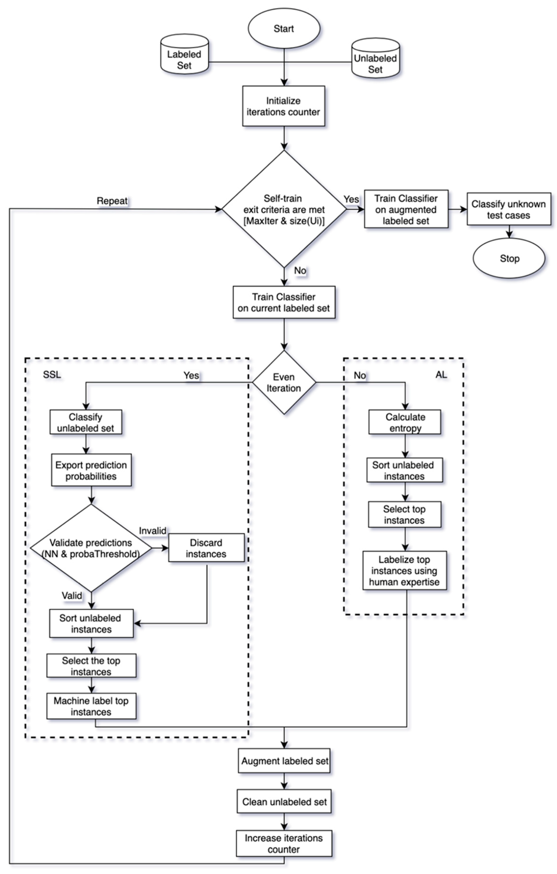
3. Proposed Method
| Algorithm 1: Combination Scheme |
|
4. Experimentation and Results
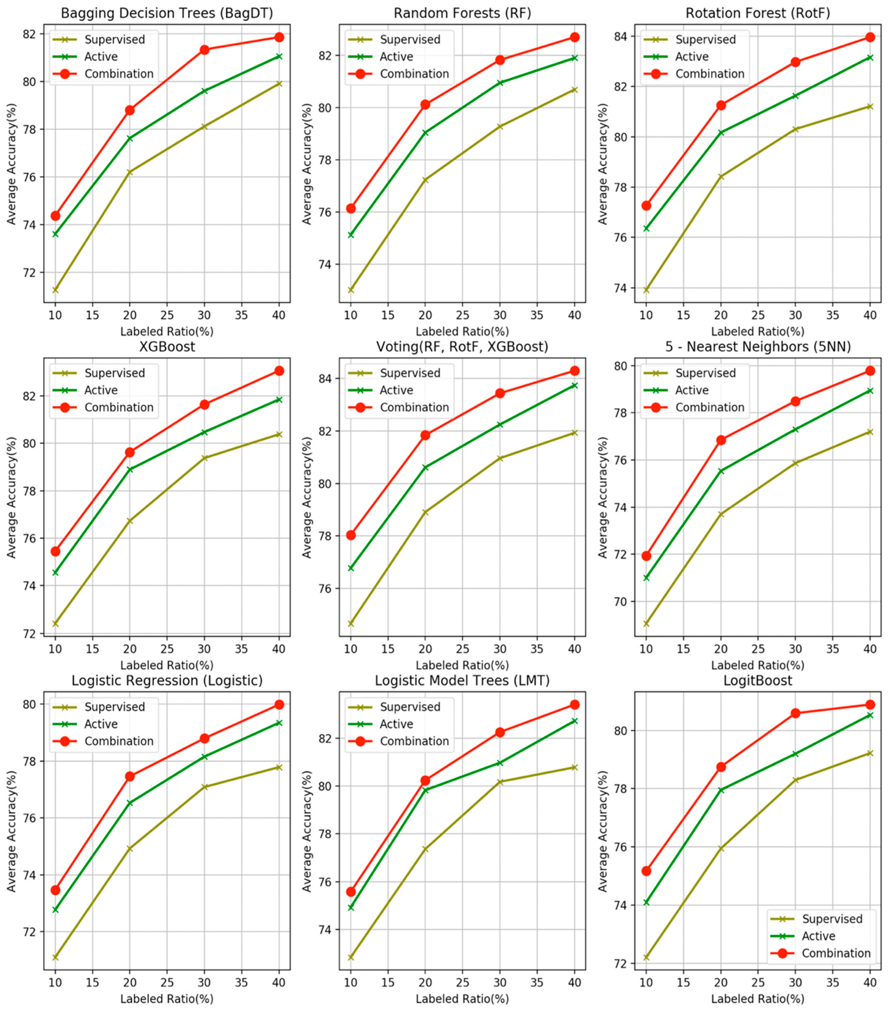
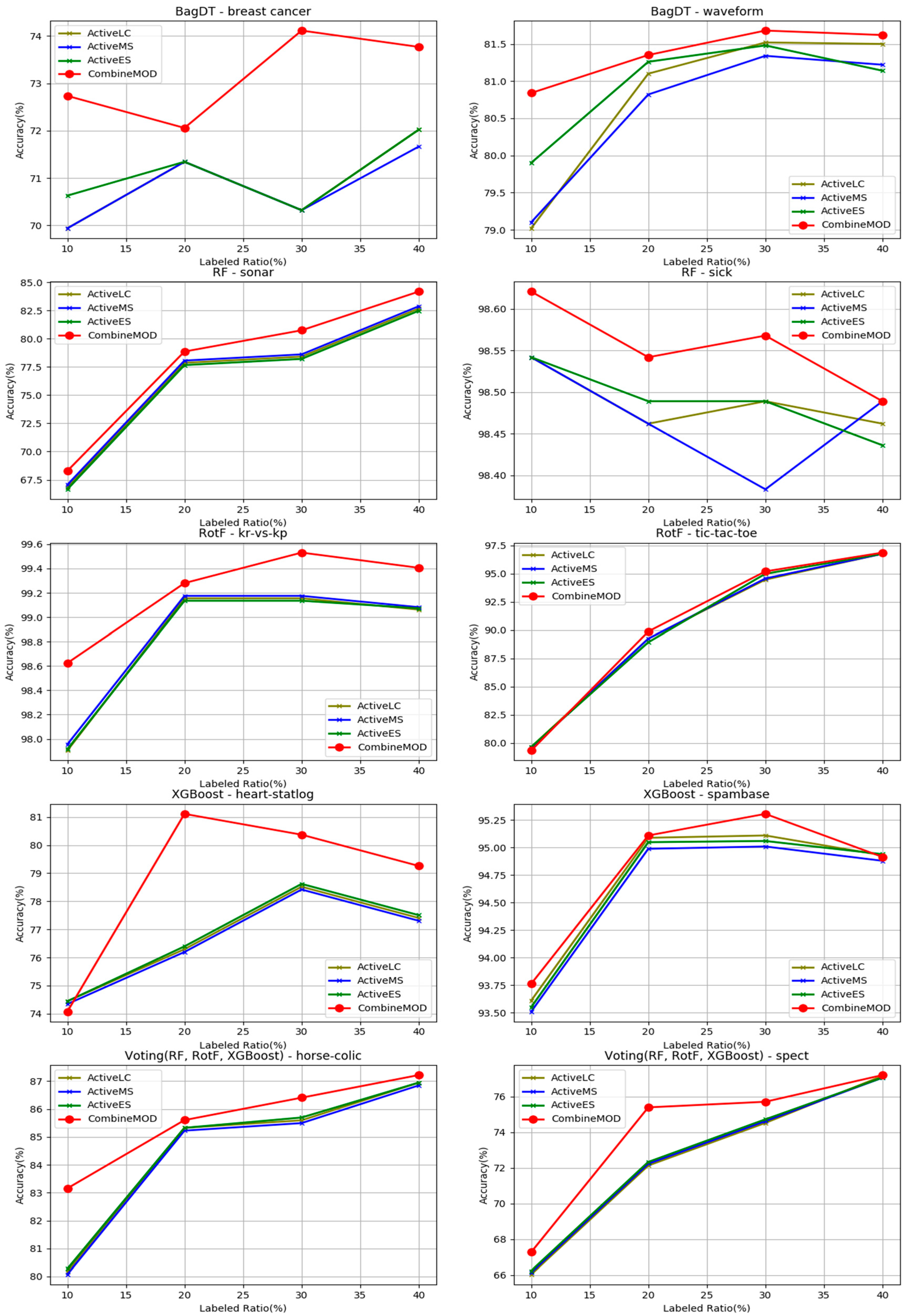
- The proposed combination method outperforms all other four learning methods in all four labeled ratios and for all the nine base learners used as control methods, in terms of average accuracy. This argument is also validated in Figure 3, where the comparisons are visually assembled and a progressive picture of the performance of the two dominant methods is presented as the R increases. The SL method was also included as a baseline performance metric.
- It is observed by the accuracy tables that the proposed method steadily produces significantly more wins on each individual dataset through all the experiments carried out.
- The non-parametric tests assess the null hypothesis that the means of the results of two or more of the compared methods are the same by calculating the related p-value. This hypothesis can be rejected for all the nine algorithms and for all labeled ratios as all calculated p-values are significantly lower than the significance level of a = 0.10.
- Moreover, the Friedman rankings confirm that for all nine base learners and regardless of the labeled ratio, the proposed combination scheme ranks first ahead of all other learning methods in coincidence with the accuracy experimental results.
- The proposed combination method performs significantly better on 105 of the total 108 compared method variations for the nine base learners over the four labeled ratios.
- The AL methods for the Logistic, the LMT and the LogitBoost classifiers accept the mean significant difference test for one label ratio each, 30%, 20%, 40% accordingly. However, the adjusted p-values show small differences over the alpha of 0.10.
5. Modification
| Algorithm 2: SSL modification |
|
6. Conclusions
Supplementary Materials
Author Contributions
Funding
Conflicts of Interest
Appendix A
References
- Rosenberg, C.; Hebert, M.; Schneiderman, H. Semi-supervised self-training of object detection models. In Proceedings of the Seventh IEEE Workshop on Applications of Computer Vision (WACV 2005), Breckenridge, CO, USA, 5–7 January 2005. [Google Scholar]
- Karlos, S.; Fazakis, N.; Karanikola, K.; Kotsiantis, S.; Sgarbas, K. Speech Recognition Combining MFCCs and Image Features. In Lecture Notes in Computer Science (Including Subseries Lecture Notes in Artificial Intelligence and Lecture Notes in Bioinformatics); Springer: Cham, Switzerland, 2016; Volume 9811 LNCS, pp. 651–658. ISBN 9783319439570. [Google Scholar]
- Tsukada, M.; Washio, T.; Motoda, H. Automatic Web-Page Classification by Using Machine Learning Methods. In Web Intelligence: Research and Development; Springer: Berlin/Heidelberg, Germany, 2001; pp. 303–313. [Google Scholar]
- Fiscon, G.; Weitschek, E.; Cella, E.; Lo Presti, A.; Giovanetti, M.; Babakir-Mina, M.; Ciotti, M.; Ciccozzi, M.; Pierangeli, A.; Bertolazzi, P.; et al. MISSEL: A method to identify a large number of small species-specific genomic subsequences and its application to viruses classification. BioData Min. 2016, 9, 38. [Google Scholar] [CrossRef] [PubMed]
- Previtali, F.; Bertolazzi, P.; Felici, G.; Weitschek, E. A novel method and software for automatically classifying Alzheimer’s disease patients by magnetic resonance imaging analysis. Comput. Methods Programs Biomed. 2017, 143, 89–95. [Google Scholar] [CrossRef] [PubMed]
- Celli, F.; Cumbo, F.; Weitschek, E. Classification of Large DNA Methylation Datasets for Identifying Cancer Drivers. Big Data Res. 2018, 13, 21–28. [Google Scholar] [CrossRef]
- Settles, B. Active Learning Literature Survey. Mach. Learn. University of Wisconsin-Madison: Madison, WI, USA, 2009; pp. 1–43.
- Triguero, I.; García, S.; Herrera, F. Self-labeled techniques for semi-supervised learning: Taxonomy, software and empirical study. Knowl. Inf. Syst. 2015, 42, 245–284. [Google Scholar] [CrossRef]
- Mousavi, R.; Eftekhari, M.; Rahdari, F. Omni-Ensemble Learning (OEL): Utilizing Over-Bagging, Static and Dynamic Ensemble Selection Approaches for Software Defect Prediction. Int. J. Artif. Intell. Tools 2018, 27, 1850024. [Google Scholar] [CrossRef]
- Bologna, G.; Hayashi, Y. A Comparison Study on Rule Extraction from Neural Network Ensembles, Boosted Shallow Trees, and SVMs. Appl. Comput. Intell. Soft Comput. 2018, 2018, 1–20. [Google Scholar] [CrossRef]
- Hajmohammadi, M.S.; Ibrahim, R.; Selamat, A.; Fujita, H. Combination of active learning and self-training for cross-lingual sentiment classification with density analysis of unlabelled samples. Inf. Sci. 2015, 317, 67–77. [Google Scholar] [CrossRef]
- Ahsan, M.N.I.; Nahian, T.; Kafi, A.A.; Hossain, M.I.; Shah, F.M. Review spam detection using active learning. In Proceedings of the IEEE 2016 7th IEEE Annual Information Technology, Electronics and Mobile Communication Conference, Vancouver, BC, Canada, 13–15 October 2016. [Google Scholar]
- Xu, J.; Fumera, G.; Roli, F.; Zhou, Z. Training spamassassin with active semi-supervised learning. In Proceedings of the 6th Conference on Email and Anti-Spam (CEAS’09), Mountain View, CA, USA, 16–17 July 2009. [Google Scholar]
- Dua, D.; Graff, C. UCI Machine Learning Repository. Available online: https://archive.ics.uci.edu/ml/citation_policy.html (accessed on 9 October 2019).
- Cortes, C.; Vapnik, V. Support-vector networks. Mach. Learn. 1995, 20, 273–297. [Google Scholar] [CrossRef]
- Sourati, J.; Akcakaya, M.; Dy, J.; Leen, T.; Erdogmus, D. Classification Active Learning Based on Mutual Information. Entropy 2016, 18, 51. [Google Scholar] [CrossRef]
- Huang, S.J.; Jin, R.; Zhou, Z.H. Active Learning by Querying Informative and Representative Examples. IEEE Trans. Pattern Anal. Mach. Intell. 2014, 36, 1936–1949. [Google Scholar] [CrossRef]
- Lewis, D.D.; Gale, W.A. A Sequential Algorithm for Training Text Classifiers. In Proceedings of the ACM SIGIR Forum, Dublin, Ireland, 3–6 July 1994. [Google Scholar]
- Riccardi, G.; Hakkani-Tür, D. Active learning: Theory and applications to automatic speech recognition. IEEE Trans. Speech Audio Process. 2005, 13, 504–511. [Google Scholar] [CrossRef]
- Zhang, Z.; Schuller, B. Active Learning by Sparse Instance Tracking and Classifier Confidence in Acoustic Emotion Recognition. In Proceedings of the Interspeech 2012, Portland, OR, USA, 9–13 September 2012. [Google Scholar]
- Roma, G.; Janer, J.; Herrera, P. Active learning of custom sound taxonomies in unstructured audio data. In Proceedings of the 2nd ACM International Conference on Multimedia Retrieval, Hong Kong, China, 5–8 June 2012. [Google Scholar]
- Chen, Y.; Wang, G.; Dong, S. Learning with progressive transductive support vector machine. Pattern Recognit. Lett. 2003, 24, 1845–1855. [Google Scholar] [CrossRef]
- Johnson, R.; Zhang, T. Graph-based semi-supervised learning and spectral kernel design. IEEE Trans. Inf. Theory 2008, 54, 275–288. [Google Scholar] [CrossRef]
- Anis, A.; El Gamal, A.; Avestimehr, A.S.; Ortega, A. A Sampling Theory Perspective of Graph-Based Semi-Supervised Learning. IEEE Trans. Inf. Theory 2019, 65, 2322–2342. [Google Scholar] [CrossRef]
- Culp, M.; Michailidis, G. Graph-based semisupervised learning. IEEE Trans. Pattern Anal. Mach. Intell. 2008, 30, 174–179. [Google Scholar] [CrossRef] [PubMed]
- Blum, A.; Mitchell, T. Combining Labeled and Unlabeled Data with Co-Training. In Proceedings of the Eleventh Annual Conference on Computational Learning Theory, Madison, WI, USA, 24–26 July 1998. [Google Scholar]
- McCallum, A.K.; Nigam, K.; McCallumzy, A.K.; Nigamy, K. Employing EM and pool-based active learning for text classification. In Proceedings of the Fifteenth International Conference on Machine Learning, Madison, WI, USA, 24–27 July 1998; pp. 359–367. [Google Scholar]
- Tur, G.; Hakkani-Tür, D.; Schapire, R.E. Combining active and semi-supervised learning for spoken language understanding. Speech Commun. 2005, 45, 171–186. [Google Scholar] [CrossRef]
- Tomanek, K.; Hahn, U. Semi-supervised active learning for sequence labeling. In Proceedings of the Joint Conference of the 47th Annual Meeting of the ACL and the 4th International Joint Conference on Natural Language Processing of the AFNLP: Volume 2, Singapore, 2–7 August 2009. [Google Scholar]
- Han, W.; Coutinho, E.; Ruan, H.; Li, H.; Schuller, B.; Yu, X.; Zhu, X. Semi-supervised active learning for sound classification in hybrid learning environments. PLoS ONE 2016, 11, e0162075. [Google Scholar] [CrossRef] [PubMed]
- Chai, H.; Liang, Y.; Wang, S.; Shen, H.-W. A novel logistic regression model combining semi-supervised learning and active learning for disease classification. Sci. Rep. 2018, 8, 13009. [Google Scholar] [CrossRef] [PubMed]
- Su, H.; Yin, Z.; Huh, S.; Kanade, T.; Zhu, J. Interactive Cell Segmentation Based on Active and Semi-Supervised Learning. IEEE Trans. Med. Imaging 2016, 35, 762–777. [Google Scholar] [CrossRef] [PubMed]
- Rhee, P.K.; Erdenee, E.; Kyun, S.D.; Ahmed, M.U.; Jin, S. Active and semi-supervised learning for object detection with imperfect data. Cogn. Syst. Res. 2017, 45, 109–123. [Google Scholar] [CrossRef]
- Yang, Y.; Loog, M. Active learning using uncertainty information. In Proceedings of the International Conference on Pattern Recognition, Cancun, Mexico, 4–8 December 2016. [Google Scholar]
- Fazakis, N.; Karlos, S.; Kotsiantis, S.; Sgarbas, K. Self-trained Rotation Forest for semi-supervised learning. J. Intell. Fuzzy Syst. 2017, 32, 711–722. [Google Scholar] [CrossRef]
- Yang, Y.; Loog, M. A benchmark and comparison of active learning for logistic regression. Pattern Recognit. 2018, 83, 401–415. [Google Scholar] [CrossRef]
- Stone, M. Cross-validation: A review. Ser. Stat. 1978, 9, 127–139. [Google Scholar] [CrossRef]
- Breiman, L. Bagging predictors. Mach. Learn. 1996, 24, 123–140. [Google Scholar] [CrossRef]
- Salzberg, S.L. C4.5: Programs for Machine Learning by J. Ross Quinlan. Morgan Kaufmann Publishers, Inc., 1993. Mach. Learn. 1994, 16, 235–240. [Google Scholar] [CrossRef]
- Aha, D.W.; Kibler, D.; Albert, M.K. Instance-Based Learning Algorithms. Mach. Learn. 1991, 6, 37–66. [Google Scholar] [CrossRef]
- Le Cessie, S.; Houwelingen, J.C. Van Ridge Estimators in Logistic Regression. Appl. Stat. 1992, 41, 191–201. [Google Scholar] [CrossRef]
- Landwehr, N.; Hall, M.; Frank, E. Logistic model trees. Mach. Learn. 2005, 59, 161–205. [Google Scholar] [CrossRef]
- Friedman, J.; Hastie, T.; Tibshirani, R. Additive logistic regression: A statistical view of boosting. Ann. Stat. 2000, 28, 337–407. [Google Scholar] [CrossRef]
- Schapire, R.E. A Short Introduction to Boosting. J. Jpn. Soc. Artif. Intell. 1999, 14, 771–780. [Google Scholar]
- Breiman, L. Random Forests. Mach. Learn. 2001, 45, 5–32. [Google Scholar] [CrossRef]
- Opitz, D.; Maclin, R. Popular Ensemble Methods: An Empirical Study. J. Artif. Intell. Res. 1999, 11, 169–198. [Google Scholar] [CrossRef]
- Rodriguez, J.J.; Kuncheva, L.I.; Alonso, C.J. Rotation forest: A new classifier ensemble method. IEEE Trans. Pattern Anal. Mach. Intell. 2006, 28, 1619–1630. [Google Scholar] [CrossRef] [PubMed]
- Han, J.; Kamber, M.; Pei, J. Data Mining: Concepts and Techniques; Elsevier: Amsterdam, The Netherlands, 2011. [Google Scholar]
- Chen, T.; Guestrin, C. XGBoost: Reliable Large-scale Tree Boosting System. Available online: http://learningsys.org/papers/LearningSys_2015_paper_32.pdf (accessed on 9 October 2019).
- Ferreira, A.J.; Figueiredo, M.A.T. Boosting algorithms: A review of methods, theory, and applications. In Ensemble Machine Learning: Methods and Applications; Springer: Boston, MA, USA, 2012. [Google Scholar]
- Friedman, M. The Use of Ranks to Avoid the Assumption of Normality Implicit in the Analysis of Variance. J. Am. Stat. Assoc. 1937, 32, 69–73. [Google Scholar] [CrossRef]
- Holm, S. A simple sequentially rejective multiple test procedure. Scand. J. Stat. 1979, 6, 65–70. [Google Scholar]
- Fazakis, N.; Karlos, S.; Kotsiantis, S.; Sgarbas, K. A multi-scheme semi-supervised regression approach. Pattern Recognit. Lett. 2019, 125, 758–765. [Google Scholar] [CrossRef]
- Culotta, A.; McCallum, A. Reducing labeling effort for structured prediction tasks. In Proceedings of the National Conference on Artificial Intelligence, Pittsburgh, PA, USA, 9–13 July 2005. [Google Scholar]
- Scheffer, T.; Decomain, C.; Wrobel, S. Active hidden markov models for information extraction. In Lecture Notes in Computer Science (including subseries Lecture Notes in Artificial Intelligence and Lecture Notes in Bioinformatics); Springer: Berlin/Heidelberg, Germany, 2001. [Google Scholar]
- Wang, L.; Hu, X.; Yuan, B.; Lu, J. Active learning via query synthesis and nearest neighbour search. Neurocomputing 2015, 147, 426–434. [Google Scholar] [CrossRef]
- Huu, Q.N.; Viet, D.C.; Thuy, Q.D.T.; Quoc, T.N.; Van, C.P. Graph-based semisupervised and manifold learning for image retrieval with SVM-based relevant feedback. J. Intell. Fuzzy Syst. 2019, 37, 711–722. [Google Scholar] [CrossRef]
- Wang, W.; Lu, P. An efficient switching median filter based on local outlier factor. IEEE Signal Process. Lett. 2011, 18, 551–554. [Google Scholar] [CrossRef]
- Liu, F.T.; Ting, K.M.; Zhou, Z.-H. Isolation forest. In Proceedings of the 2008 Eighth IEEE International Conference on Data Mining, Pisa, Italy, 15–19 December 2008; pp. 413–422. [Google Scholar]
- Tang, J.; Alelyani, S.; Liu, H. Feature selection for classification: A review. In Data Classification: Algorithms and Applications; CRC Press: Boca Raton, FL, USA, 2014. [Google Scholar]
- Hulten, G.; Spencer, L.; Domingos, P. Mining time-changing data streams. In Proceedings of the Seventh ACM SIGKDD International Conference on Knowledge Discovery and data Mining KDD ’01, San Francisco, CA, USA, 26–29 August 2001. [Google Scholar]
- Shalev-Shwartz, S.; Singer, Y.; Srebro, N.; Cotter, A. Pegasos: Primal estimated sub-gradient solver for SVM. Math. Program. 2011, 127, 3–30. [Google Scholar] [CrossRef]
- Liu, W.; Wang, Z.; Liu, X.; Zeng, N.; Liu, Y.; Alsaadi, F.E. A survey of deep neural network architectures and their applications. Neurocomputing 2017, 234, 11–26. [Google Scholar] [CrossRef]
- Amini, M.; Rezaeenour, J.; Hadavandi, E. A Neural Network Ensemble Classifier for Effective Intrusion Detection Using Fuzzy Clustering and Radial Basis Function Networks. Int. J. Artif. Intell. Tools 2016, 25, 1550033. [Google Scholar] [CrossRef]
- Elreedy, D.; Atiya, A.F.; Shaheen, S.I. A Novel Active Learning Regression Framework for Balancing the Exploration-Exploitation Trade-Off. Entropy 2019, 21, 651. [Google Scholar] [CrossRef]
- Fazakis, N.; Kostopoulos, G.; Karlos, S.; Kotsiantis, S.; Sgarbas, K. An Active Learning Ensemble Method for Regression Tasks. Intell. Data Anal. 2020, 24. [Google Scholar] [CrossRef]
- Hall, M.; Frank, E.; Holmes, G.; Pfahringer, B.; Reutemann, P.; Witten, I.H. The WEKA data mining software. ACM SIGKDD Explor. Newsl. 2009, 11, 10. [Google Scholar] [CrossRef]


| R = 10% | R = 20% | R = 30% | R = 40% | ||||||||||||||
|---|---|---|---|---|---|---|---|---|---|---|---|---|---|---|---|---|---|
| Method | Supervised | Semi-Supervised | Active Random | Combination | Supervised | Semi-Supervised | Active Random | Combination | Supervised | Semi-Supervised | Active Random | Combination | Supervised | Semi-Supervised | Active Random | Combination | |
| Dataset | |||||||||||||||||
| anneal | 88.866 | 88.524 | 93.211 | 94.660 | 95.210 | 95.988 | 96.770 | 99.107 | 96.659 | 96.547 | 97.551 | 98.663 | 97.773 | 97.215 | 98.326 | 98.885 | |
| arrhythmia | 58.425 | 57.981 | 62.614 | 63.285 | 65.063 | 63.314 | 68.807 | 69.691 | 70.140 | 70.589 | 69.483 | 70.812 | 70.348 | 69.498 | 73.242 | 73.464 | |
| audiology | 52.253 | 50.474 | 56.166 | 56.640 | 61.087 | 61.482 | 65.593 | 68.636 | 65.138 | 64.684 | 73.004 | 74.308 | 71.660 | 70.791 | 75.178 | 80.079 | |
| autos | 45.381 | 44.286 | 50.167 | 48.286 | 52.119 | 56.167 | 61.000 | 55.619 | 60.976 | 58.143 | 63.405 | 66.381 | 65.405 | 59.048 | 69.738 | 72.690 | |
| balance-scale | 73.103 | 75.832 | 74.560 | 75.996 | 76.487 | 75.540 | 80.476 | 81.608 | 81.129 | 78.571 | 81.941 | 81.764 | 83.372 | 78.093 | 83.518 | 83.372 | |
| breast-cancer | 69.926 | 70.628 | 70.603 | 69.544 | 69.963 | 70.616 | 70.603 | 70.961 | 70.961 | 70.616 | 70.591 | 71.675 | 71.293 | 70.616 | 70.948 | 74.803 | |
| bridges-version1 | 45.727 | 45.727 | 45.727 | 45.727 | 53.273 | 57.909 | 57.273 | 56.909 | 60.000 | 60.727 | 60.000 | 62.455 | 61.000 | 61.091 | 64.909 | 62.909 | |
| bridges-version2 | 43.000 | 43.000 | 43.000 | 43.000 | 48.455 | 51.091 | 59.818 | 53.909 | 60.000 | 64.000 | 63.091 | 62.818 | 62.091 | 59.182 | 63.636 | 62.000 | |
| clevalend | 78.215 | 76.559 | 75.849 | 75.559 | 73.247 | 74.570 | 79.204 | 78.194 | 79.516 | 76.839 | 80.462 | 81.484 | 83.151 | 78.516 | 80.495 | 81.806 | |
| cmc | 48.066 | 48.329 | 49.356 | 49.691 | 50.302 | 51.455 | 54.307 | 51.260 | 50.576 | 52.339 | 51.527 | 53.154 | 53.220 | 54.100 | 52.674 | 53.428 | |
| column_2C | 76.452 | 75.806 | 75.806 | 80.645 | 80.323 | 80.323 | 80.323 | 84.516 | 81.613 | 80.968 | 82.258 | 82.903 | 82.258 | 82.258 | 82.903 | 83.226 | |
| column_3C | 79.032 | 79.032 | 77.419 | 77.742 | 79.355 | 78.710 | 79.677 | 83.226 | 80.323 | 80.645 | 78.065 | 83.871 | 79.355 | 79.032 | 82.258 | 82.903 | |
| credit-rating | 84.783 | 83.768 | 85.217 | 85.362 | 84.638 | 84.783 | 85.217 | 85.507 | 85.652 | 85.507 | 85.652 | 86.667 | 85.072 | 85.942 | 86.087 | 86.232 | |
| cylinder-bands | 58.333 | 57.037 | 57.222 | 59.444 | 59.630 | 60.000 | 59.259 | 60.556 | 58.889 | 58.704 | 58.148 | 59.074 | 60.556 | 57.963 | 58.519 | 59.259 | |
| dermatology | 71.089 | 70.578 | 82.770 | 87.447 | 84.977 | 83.348 | 91.036 | 95.931 | 91.006 | 91.029 | 93.483 | 95.113 | 93.461 | 89.647 | 92.658 | 96.742 | |
| ecoli | 67.282 | 68.173 | 76.471 | 76.194 | 79.144 | 76.185 | 80.936 | 81.230 | 80.936 | 80.963 | 81.827 | 83.324 | 80.348 | 79.162 | 83.324 | 83.316 | |
| flags | 50.053 | 48.553 | 48.526 | 49.921 | 51.105 | 51.079 | 52.026 | 52.579 | 55.658 | 52.184 | 51.132 | 56.763 | 56.237 | 52.605 | 55.289 | 52.711 | |
| german_credit | 70.500 | 69.200 | 69.300 | 70.800 | 70.900 | 69.200 | 69.500 | 71.400 | 69.500 | 70.500 | 74.000 | 74.000 | 73.600 | 71.800 | 72.500 | 73.000 | |
| glass | 50.498 | 47.684 | 51.991 | 53.810 | 64.524 | 59.848 | 57.468 | 65.952 | 60.303 | 60.779 | 67.727 | 67.338 | 69.113 | 64.372 | 67.229 | 69.113 | |
| haberman | 72.538 | 71.591 | 71.559 | 70.882 | 72.860 | 73.204 | 70.882 | 73.860 | 71.871 | 72.538 | 72.204 | 73.194 | 71.871 | 71.538 | 71.839 | 71.237 | |
| heart-statlog | 72.963 | 71.481 | 74.444 | 75.185 | 75.556 | 77.037 | 78.148 | 80.741 | 77.778 | 76.667 | 80.370 | 84.074 | 79.630 | 77.037 | 82.222 | 82.963 | |
| hepatitis | 80.083 | 81.958 | 79.375 | 81.917 | 78.792 | 80.083 | 80.000 | 81.875 | 82.542 | 82.542 | 79.958 | 79.417 | 82.542 | 80.000 | 78.000 | 79.875 | |
| horse-colic | 78.551 | 78.544 | 82.605 | 84.219 | 84.775 | 83.138 | 82.868 | 85.308 | 83.401 | 82.590 | 84.219 | 85.300 | 83.949 | 85.030 | 85.571 | 85.841 | |
| hungarian-heart | 81.000 | 78.632 | 78.310 | 82.391 | 81.023 | 80.701 | 78.276 | 78.966 | 78.621 | 78.644 | 78.977 | 83.057 | 76.897 | 76.885 | 81.655 | 79.310 | |
| hypothyroid | 98.357 | 98.199 | 98.808 | 99.602 | 99.072 | 98.887 | 99.046 | 99.602 | 99.099 | 99.099 | 99.417 | 99.549 | 99.285 | 99.311 | 99.443 | 99.576 | |
| ionosphere | 75.802 | 77.802 | 86.643 | 84.667 | 88.040 | 88.032 | 88.333 | 92.317 | 86.619 | 86.357 | 91.183 | 92.317 | 90.611 | 89.746 | 90.611 | 92.032 | |
| iris | 72.667 | 77.333 | 84.667 | 86.667 | 88.000 | 89.333 | 90.667 | 90.667 | 93.333 | 93.333 | 91.333 | 92.000 | 93.333 | 93.333 | 93.333 | 92.667 | |
| kr-vs-kp | 95.025 | 95.244 | 96.340 | 98.499 | 97.027 | 97.310 | 98.091 | 99.249 | 97.998 | 98.216 | 98.748 | 99.343 | 98.998 | 98.811 | 99.218 | 99.343 | |
| labor | 66.333 | 66.333 | 66.333 | 66.333 | 65.667 | 70.333 | 70.000 | 66.333 | 70.000 | 73.667 | 77.000 | 87.667 | 77.000 | 79.000 | 78.667 | 79.000 | |
| letter | 77.955 | 77.235 | 81.320 | 84.490 | 83.775 | 82.470 | 86.570 | 89.840 | 86.570 | 85.770 | 89.165 | 92.175 | 88.335 | 86.375 | 90.280 | 92.620 | |
| lymphography | 65.476 | 66.143 | 68.952 | 67.619 | 77.571 | 72.381 | 71.571 | 71.667 | 72.905 | 70.857 | 75.571 | 79.048 | 74.286 | 76.238 | 77.619 | 79.667 | |
| mushroom | 99.163 | 99.323 | 99.729 | 100.000 | 99.877 | 99.889 | 99.914 | 100.000 | 99.951 | 99.902 | 99.975 | 100.000 | 99.963 | 99.975 | 99.975 | 100.000 | |
| optdigits | 89.021 | 86.174 | 90.783 | 92.829 | 92.189 | 90.036 | 93.043 | 95.979 | 92.936 | 90.587 | 93.719 | 95.712 | 94.288 | 90.854 | 94.555 | 95.498 | |
| page-blocks | 95.414 | 95.468 | 95.980 | 97.058 | 96.236 | 95.926 | 96.547 | 97.113 | 96.620 | 96.583 | 97.369 | 97.241 | 97.168 | 97.004 | 97.150 | 97.168 | |
| pendigits | 93.122 | 92.849 | 94.796 | 96.516 | 95.515 | 94.860 | 96.061 | 97.862 | 96.179 | 96.006 | 96.871 | 98.335 | 96.880 | 96.243 | 97.362 | 98.071 | |
| pima_diabetes | 71.880 | 73.055 | 75.135 | 74.479 | 75.911 | 73.970 | 74.747 | 73.445 | 75.270 | 75.261 | 73.841 | 76.307 | 76.309 | 76.044 | 74.498 | 75.930 | |
| postoperative | 65.556 | 65.556 | 65.556 | 65.556 | 67.778 | 71.111 | 64.444 | 66.667 | 62.222 | 67.778 | 66.667 | 67.778 | 64.444 | 67.778 | 65.556 | 67.778 | |
| primary-tumor | 29.474 | 30.339 | 35.954 | 34.795 | 35.651 | 34.750 | 38.610 | 36.248 | 38.610 | 34.198 | 37.745 | 37.469 | 40.401 | 35.677 | 41.578 | 38.930 | |
| segment | 90.736 | 90.779 | 91.472 | 94.329 | 93.420 | 93.117 | 94.372 | 97.229 | 93.853 | 94.502 | 95.455 | 97.359 | 94.589 | 94.892 | 96.017 | 97.186 | |
| sick | 97.640 | 97.587 | 97.932 | 98.648 | 98.038 | 98.118 | 98.117 | 98.754 | 98.118 | 98.144 | 98.223 | 98.728 | 98.277 | 98.144 | 98.595 | 98.621 | |
| solar-flare | 67.914 | 64.807 | 68.439 | 68.164 | 69.790 | 68.941 | 70.081 | 70.322 | 70.115 | 70.538 | 71.532 | 71.260 | 70.336 | 71.536 | 71.448 | 71.905 | |
| sonar | 59.524 | 60.976 | 64.881 | 60.548 | 66.833 | 64.429 | 68.714 | 67.881 | 69.214 | 70.595 | 74.048 | 71.119 | 70.714 | 69.214 | 76.476 | 75.024 | |
| soybean | 64.241 | 61.624 | 75.980 | 70.119 | 79.211 | 75.835 | 84.633 | 86.091 | 84.486 | 82.564 | 87.551 | 90.635 | 86.520 | 84.318 | 91.355 | 93.116 | |
| spambase | 89.937 | 90.285 | 90.545 | 92.827 | 91.328 | 91.784 | 92.349 | 94.305 | 92.132 | 92.827 | 92.805 | 94.631 | 92.741 | 92.067 | 93.219 | 94.610 | |
| spect | 61.316 | 61.494 | 61.864 | 63.367 | 68.506 | 65.344 | 66.099 | 66.902 | 66.717 | 71.978 | 73.390 | 80.342 | 79.186 | 74.895 | 77.025 | 76.084 | |
| sponge | 86.250 | 86.250 | 86.250 | 86.250 | 91.071 | 92.500 | 92.500 | 92.500 | 92.500 | 92.500 | 92.500 | 92.500 | 93.750 | 92.500 | 92.500 | 93.750 | |
| tae | 32.375 | 34.375 | 40.417 | 38.375 | 38.333 | 36.958 | 38.333 | 41.000 | 42.958 | 41.708 | 40.333 | 52.250 | 44.375 | 42.333 | 53.583 | 54.875 | |
| tic-tac-toe | 70.254 | 70.985 | 74.221 | 76.620 | 78.189 | 74.326 | 80.895 | 83.091 | 82.467 | 76.404 | 84.864 | 86.951 | 84.444 | 80.684 | 89.457 | 91.864 | |
| vehicle | 64.189 | 62.289 | 67.150 | 67.615 | 66.916 | 67.134 | 70.445 | 69.618 | 70.221 | 70.091 | 73.175 | 71.161 | 73.060 | 70.454 | 72.108 | 72.696 | |
| vote | 94.049 | 94.952 | 94.276 | 95.174 | 95.412 | 95.418 | 94.049 | 96.321 | 95.412 | 95.640 | 96.327 | 95.872 | 95.640 | 95.645 | 96.781 | 96.327 | |
| vowel | 48.283 | 49.192 | 52.424 | 54.040 | 60.808 | 60.707 | 67.980 | 70.202 | 70.707 | 65.758 | 74.545 | 77.172 | 73.939 | 68.485 | 80.303 | 83.737 | |
| waveform | 78.020 | 75.600 | 79.180 | 79.700 | 80.300 | 77.540 | 79.160 | 81.340 | 79.160 | 78.380 | 81.200 | 81.260 | 80.700 | 78.160 | 80.880 | 81.740 | |
| wine | 74.314 | 78.203 | 80.425 | 84.935 | 88.758 | 85.425 | 91.601 | 93.268 | 90.458 | 89.379 | 93.301 | 96.078 | 92.157 | 91.601 | 92.712 | 94.379 | |
| wisconsin-breast | 91.986 | 92.418 | 92.416 | 95.422 | 94.559 | 93.704 | 94.994 | 96.422 | 95.565 | 94.277 | 95.565 | 95.994 | 94.996 | 95.277 | 95.137 | 96.137 | |
| zoo | 57.455 | 57.455 | 57.455 | 57.455 | 75.273 | 75.273 | 78.273 | 85.182 | 81.273 | 82.273 | 86.273 | 88.273 | 84.273 | 86.273 | 88.273 | 93.182 | |
| Average | 71.270 | 71.158 | 73.611 | 74.383 | 76.216 | 75.847 | 77.631 | 78.817 | 78.125 | 77.863 | 79.614 | 81.348 | 79.913 | 78.623 | 81.062 | 81.867 | |
| R = 10% | R = 20% | R = 30% | R = 40% | ||||||||||||||
|---|---|---|---|---|---|---|---|---|---|---|---|---|---|---|---|---|---|
| Method | Supervised | Semi-Supervised | Active Random | Combination | Supervised | Semi-Supervised | Active Random | Combination | Supervised | Semi-Supervised | Active Random | Combination | Supervised | Semi-Supervised | Active Random | Combination | |
| Dataset | |||||||||||||||||
| anneal | 83.740 | 83.965 | 85.414 | 87.976 | 87.418 | 87.194 | 90.979 | 92.203 | 90.869 | 90.087 | 92.985 | 93.762 | 92.875 | 92.427 | 93.871 | 94.871 | |
| arrhythmia | 56.638 | 56.633 | 60.406 | 60.623 | 59.720 | 58.841 | 60.396 | 64.599 | 59.285 | 58.184 | 63.275 | 64.821 | 62.377 | 59.517 | 63.937 | 65.488 | |
| audiology | 42.490 | 36.739 | 53.518 | 45.652 | 56.700 | 54.466 | 63.794 | 59.308 | 61.976 | 63.241 | 72.134 | 68.617 | 68.123 | 67.767 | 73.874 | 73.379 | |
| autos | 48.833 | 49.714 | 52.119 | 51.238 | 56.929 | 57.452 | 65.381 | 66.286 | 68.286 | 69.262 | 70.667 | 74.595 | 68.738 | 69.738 | 77.976 | 79.476 | |
| balance-scale | 78.067 | 77.588 | 79.027 | 80.461 | 79.519 | 78.241 | 79.841 | 80.161 | 82.084 | 79.524 | 82.087 | 81.935 | 82.081 | 80.806 | 81.910 | 81.129 | |
| breast-cancer | 69.249 | 70.283 | 67.131 | 72.044 | 67.180 | 68.559 | 64.310 | 68.276 | 66.773 | 68.153 | 67.192 | 66.441 | 67.106 | 69.212 | 64.754 | 68.596 | |
| bridges-version1 | 44.636 | 44.636 | 44.636 | 44.636 | 44.636 | 38.000 | 46.545 | 44.727 | 46.636 | 44.545 | 52.545 | 45.545 | 51.545 | 45.545 | 52.273 | 55.000 | |
| bridges-version2 | 41.818 | 41.818 | 41.818 | 41.818 | 45.545 | 37.000 | 49.273 | 46.455 | 48.364 | 40.000 | 53.182 | 45.545 | 53.273 | 47.545 | 53.182 | 52.273 | |
| clevalend | 76.849 | 75.172 | 79.505 | 78.817 | 80.161 | 79.495 | 83.430 | 81.108 | 81.086 | 79.774 | 82.806 | 81.774 | 82.452 | 82.108 | 83.774 | 81.806 | |
| cmc | 48.881 | 48.406 | 50.102 | 48.401 | 49.964 | 51.322 | 51.798 | 50.239 | 51.525 | 51.730 | 50.914 | 52.544 | 51.116 | 52.000 | 50.908 | 52.200 | |
| column_2C | 77.097 | 76.774 | 77.419 | 79.355 | 80.000 | 79.677 | 80.968 | 81.290 | 81.935 | 81.935 | 83.548 | 83.871 | 83.871 | 81.613 | 82.581 | 85.484 | |
| column_3C | 77.742 | 79.032 | 79.677 | 82.258 | 82.903 | 82.258 | 84.516 | 82.903 | 82.581 | 83.226 | 81.290 | 84.839 | 81.935 | 82.258 | 81.290 | 84.194 | |
| credit-rating | 82.319 | 82.464 | 83.478 | 85.217 | 83.768 | 84.203 | 84.493 | 85.797 | 83.768 | 84.203 | 84.928 | 85.362 | 84.638 | 84.348 | 84.783 | 86.087 | |
| cylinder-bands | 59.259 | 58.519 | 63.333 | 64.259 | 65.185 | 59.444 | 67.778 | 65.741 | 67.593 | 60.185 | 70.185 | 70.000 | 67.222 | 60.000 | 71.296 | 70.185 | |
| dermatology | 78.709 | 79.797 | 86.877 | 92.598 | 90.961 | 89.595 | 94.805 | 95.616 | 93.716 | 93.724 | 95.090 | 96.456 | 95.638 | 94.264 | 93.986 | 96.179 | |
| ecoli | 74.091 | 72.906 | 77.674 | 78.574 | 80.339 | 77.968 | 84.189 | 84.777 | 84.189 | 80.651 | 84.225 | 85.695 | 83.307 | 84.216 | 85.410 | 86.292 | |
| flags | 46.447 | 41.789 | 44.395 | 48.421 | 52.763 | 38.711 | 52.711 | 51.053 | 54.737 | 45.921 | 50.132 | 52.184 | 54.289 | 47.000 | 57.789 | 52.132 | |
| german_credit | 72.900 | 72.200 | 73.300 | 72.700 | 74.000 | 73.600 | 73.900 | 75.600 | 73.900 | 73.700 | 75.300 | 75.300 | 74.900 | 71.600 | 74.500 | 75.400 | |
| glass | 55.216 | 53.333 | 57.987 | 55.216 | 66.385 | 66.840 | 68.701 | 68.247 | 68.723 | 69.156 | 71.948 | 75.714 | 72.381 | 67.706 | 74.762 | 74.286 | |
| haberman | 62.043 | 65.656 | 66.344 | 64.258 | 68.591 | 69.903 | 67.269 | 68.581 | 66.978 | 67.634 | 66.355 | 69.237 | 67.022 | 68.989 | 66.301 | 66.677 | |
| heart-statlog | 74.074 | 75.185 | 74.815 | 77.037 | 78.519 | 78.519 | 78.148 | 81.111 | 79.259 | 78.519 | 81.481 | 83.333 | 80.741 | 78.889 | 82.222 | 81.852 | |
| hepatitis | 80.667 | 80.708 | 80.125 | 83.792 | 78.167 | 79.458 | 81.250 | 83.125 | 82.000 | 82.542 | 78.667 | 84.458 | 81.917 | 81.875 | 78.667 | 85.125 | |
| horse-colic | 79.069 | 79.595 | 79.857 | 82.590 | 84.227 | 83.664 | 83.949 | 84.767 | 83.686 | 82.057 | 84.219 | 85.578 | 83.941 | 85.856 | 84.767 | 86.119 | |
| hungarian-heart | 79.276 | 79.264 | 79.989 | 82.000 | 83.046 | 83.046 | 81.000 | 82.011 | 81.345 | 81.345 | 80.287 | 81.000 | 81.644 | 81.655 | 81.299 | 80.966 | |
| hypothyroid | 95.733 | 95.520 | 96.660 | 99.258 | 97.880 | 97.429 | 98.569 | 99.444 | 98.330 | 98.039 | 98.966 | 99.391 | 98.993 | 98.596 | 98.914 | 99.364 | |
| ionosphere | 81.802 | 80.381 | 86.929 | 88.603 | 90.603 | 89.746 | 90.889 | 92.889 | 91.460 | 90.603 | 92.889 | 93.460 | 91.746 | 91.746 | 93.175 | 94.032 | |
| iris | 83.333 | 83.333 | 88.000 | 90.000 | 93.333 | 92.000 | 96.000 | 94.667 | 96.000 | 95.333 | 96.000 | 94.667 | 95.333 | 95.333 | 94.667 | 95.333 | |
| kr-vs-kp | 95.776 | 94.900 | 96.120 | 98.623 | 96.778 | 96.621 | 97.497 | 99.280 | 97.559 | 97.465 | 98.248 | 99.406 | 98.154 | 98.216 | 98.937 | 99.312 | |
| labor | 65.000 | 65.000 | 65.000 | 65.000 | 73.667 | 69.667 | 82.000 | 80.333 | 82.000 | 77.000 | 84.000 | 82.667 | 84.000 | 73.333 | 82.667 | 82.333 | |
| letter | 84.795 | 84.210 | 87.940 | 90.915 | 89.845 | 89.625 | 92.215 | 95.300 | 92.215 | 91.870 | 94.050 | 96.290 | 93.415 | 92.955 | 95.010 | 96.435 | |
| lymphography | 68.238 | 67.571 | 73.619 | 75.000 | 74.190 | 76.286 | 77.619 | 76.238 | 74.333 | 76.333 | 81.667 | 80.333 | 79.048 | 77.619 | 85.143 | 85.095 | |
| mushroom | 99.741 | 99.766 | 99.914 | 100.000 | 99.963 | 99.963 | 100.000 | 100.000 | 99.988 | 99.988 | 99.975 | 100.000 | 100.000 | 99.988 | 100.000 | 100.000 | |
| optdigits | 94.573 | 94.431 | 95.765 | 97.473 | 96.406 | 96.050 | 97.011 | 98.327 | 97.135 | 96.762 | 97.438 | 98.327 | 97.438 | 96.886 | 97.865 | 98.363 | |
| page-blocks | 95.870 | 95.797 | 96.218 | 97.351 | 96.492 | 96.455 | 96.675 | 97.497 | 96.748 | 96.766 | 97.004 | 97.552 | 96.985 | 96.912 | 97.479 | 97.533 | |
| pendigits | 97.143 | 96.980 | 97.607 | 98.463 | 98.008 | 97.844 | 98.317 | 99.236 | 98.372 | 98.353 | 98.772 | 99.245 | 98.672 | 98.435 | 98.917 | 99.172 | |
| pima_diabetes | 74.354 | 72.404 | 74.231 | 74.612 | 75.656 | 74.614 | 75.921 | 76.304 | 77.092 | 76.832 | 75.930 | 74.879 | 75.531 | 75.138 | 74.624 | 76.048 | |
| postoperative | 68.889 | 68.889 | 68.889 | 68.889 | 62.222 | 66.667 | 62.222 | 67.778 | 63.333 | 64.444 | 64.444 | 65.556 | 60.000 | 65.556 | 63.333 | 63.333 | |
| primary-tumor | 33.601 | 34.768 | 37.424 | 33.592 | 37.406 | 38.592 | 43.039 | 40.383 | 43.039 | 40.348 | 42.736 | 43.913 | 41.551 | 40.642 | 43.627 | 43.039 | |
| segment | 93.333 | 93.463 | 94.372 | 96.537 | 95.281 | 95.238 | 95.844 | 97.965 | 95.628 | 95.671 | 96.970 | 98.009 | 96.537 | 96.364 | 97.403 | 98.225 | |
| sick | 96.527 | 96.394 | 96.659 | 98.595 | 97.455 | 97.455 | 97.773 | 98.542 | 97.667 | 97.534 | 97.958 | 98.462 | 97.905 | 97.826 | 98.144 | 98.436 | |
| solar-flare | 66.769 | 65.990 | 69.098 | 69.375 | 70.512 | 70.059 | 70.131 | 70.464 | 70.073 | 70.037 | 69.758 | 71.550 | 70.041 | 69.681 | 70.513 | 72.590 | |
| sonar | 62.024 | 64.024 | 67.333 | 69.643 | 69.238 | 69.738 | 75.929 | 79.333 | 74.976 | 75.976 | 76.929 | 81.238 | 79.786 | 75.952 | 82.238 | 82.690 | |
| soybean | 67.199 | 64.429 | 76.281 | 75.251 | 79.066 | 77.006 | 85.211 | 87.990 | 86.816 | 84.474 | 89.744 | 92.822 | 88.286 | 88.572 | 91.360 | 93.110 | |
| spambase | 92.871 | 92.566 | 93.088 | 94.588 | 93.523 | 93.305 | 94.197 | 95.544 | 94.305 | 94.110 | 94.675 | 95.675 | 94.523 | 94.327 | 94.936 | 95.588 | |
| spect | 69.270 | 69.825 | 68.522 | 69.270 | 72.395 | 72.133 | 71.284 | 78.837 | 75.582 | 71.948 | 78.159 | 79.193 | 80.196 | 77.765 | 79.895 | 77.381 | |
| sponge | 92.500 | 92.500 | 92.500 | 92.500 | 92.500 | 92.500 | 92.500 | 92.500 | 92.500 | 92.500 | 92.500 | 92.500 | 93.750 | 93.750 | 92.500 | 93.750 | |
| tae | 36.375 | 37.750 | 41.750 | 41.667 | 39.708 | 37.042 | 41.667 | 43.542 | 40.375 | 39.083 | 49.042 | 49.625 | 46.333 | 45.042 | 56.333 | 57.667 | |
| tic-tac-toe | 76.512 | 74.942 | 78.396 | 83.296 | 81.735 | 80.171 | 84.343 | 91.544 | 84.240 | 81.110 | 88.515 | 95.510 | 89.764 | 82.156 | 91.549 | 96.658 | |
| vehicle | 65.132 | 64.311 | 70.339 | 69.151 | 71.761 | 70.104 | 70.227 | 73.167 | 70.340 | 70.697 | 74.115 | 73.527 | 71.992 | 71.169 | 74.591 | 73.161 | |
| vote | 94.503 | 94.276 | 94.958 | 96.327 | 95.196 | 94.503 | 94.947 | 96.332 | 95.412 | 95.180 | 96.786 | 96.332 | 96.559 | 96.327 | 97.014 | 96.781 | |
| vowel | 34.444 | 33.737 | 44.848 | 42.727 | 56.566 | 55.657 | 71.313 | 71.111 | 71.010 | 69.899 | 84.545 | 88.788 | 80.808 | 80.000 | 91.616 | 96.162 | |
| waveform | 83.660 | 82.940 | 84.340 | 83.920 | 84.300 | 84.140 | 84.140 | 84.620 | 84.140 | 83.860 | 84.440 | 84.840 | 85.100 | 83.960 | 85.220 | 84.840 | |
| wine | 86.046 | 86.601 | 85.980 | 94.412 | 94.379 | 96.601 | 95.000 | 98.301 | 96.111 | 96.667 | 97.222 | 98.333 | 98.333 | 97.222 | 97.222 | 98.301 | |
| wisconsin-breast | 94.414 | 94.986 | 95.130 | 97.280 | 96.135 | 95.418 | 96.420 | 96.851 | 96.706 | 96.565 | 96.280 | 96.565 | 95.994 | 96.280 | 96.280 | 96.422 | |
| zoo | 75.273 | 75.273 | 75.273 | 75.273 | 79.273 | 77.273 | 79.273 | 88.182 | 85.273 | 79.273 | 87.273 | 93.182 | 88.273 | 84.273 | 87.273 | 92.182 | |
| Average | 73.015 | 72.730 | 75.130 | 76.137 | 77.238 | 76.316 | 79.047 | 80.118 | 79.274 | 78.255 | 80.954 | 81.826 | 80.694 | 79.436 | 81.901 | 82.701 | |
| R = 10% | R = 20% | R = 30% | R = 40% | ||||||||||||||
|---|---|---|---|---|---|---|---|---|---|---|---|---|---|---|---|---|---|
| Method | Supervised | Semi-Supervised | Active Random | Combination | Supervised | Semi-Supervised | Active Random | Combination | Supervised | Semi-Supervised | Active Random | Combination | Supervised | Semi-Supervised | Active Random | Combination | |
| Dataset | |||||||||||||||||
| anneal | 85.185 | 86.075 | 86.859 | 91.080 | 88.206 | 91.541 | 93.211 | 94.206 | 93.432 | 93.543 | 95.104 | 96.215 | 94.878 | 94.988 | 96.105 | 96.880 | |
| arrhythmia | 59.271 | 64.377 | 61.512 | 66.357 | 67.937 | 67.705 | 67.266 | 70.130 | 69.266 | 68.150 | 69.053 | 71.242 | 68.159 | 72.353 | 72.135 | 71.469 | |
| audiology | 51.759 | 51.759 | 57.589 | 58.379 | 65.929 | 63.775 | 67.312 | 70.810 | 65.949 | 67.292 | 72.095 | 74.783 | 70.296 | 70.771 | 76.482 | 79.644 | |
| autos | 47.333 | 45.405 | 54.143 | 52.262 | 53.595 | 59.405 | 66.333 | 60.857 | 66.405 | 68.214 | 69.690 | 69.762 | 68.738 | 72.643 | 75.595 | 72.643 | |
| balance-scale | 83.669 | 83.513 | 85.261 | 84.470 | 84.956 | 85.750 | 86.892 | 86.879 | 87.837 | 87.046 | 87.673 | 88.966 | 88.490 | 89.601 | 89.913 | 91.027 | |
| breast-cancer | 64.335 | 66.096 | 69.224 | 67.180 | 69.286 | 70.320 | 69.963 | 70.345 | 73.042 | 72.709 | 73.067 | 73.448 | 69.224 | 69.594 | 69.544 | 72.007 | |
| bridges-version1 | 50.455 | 50.455 | 50.455 | 50.455 | 56.091 | 53.182 | 58.091 | 51.091 | 59.273 | 65.636 | 60.182 | 63.818 | 58.182 | 64.727 | 67.727 | 60.091 | |
| bridges-version2 | 48.455 | 48.455 | 48.455 | 48.455 | 54.273 | 51.273 | 62.909 | 57.818 | 54.727 | 58.273 | 58.182 | 61.818 | 57.091 | 58.364 | 64.909 | 66.818 | |
| clevalend | 74.172 | 77.527 | 76.892 | 79.462 | 81.817 | 79.860 | 82.161 | 81.151 | 81.151 | 81.806 | 82.129 | 82.194 | 83.462 | 82.473 | 82.817 | 84.441 | |
| cmc | 49.764 | 49.968 | 49.492 | 49.899 | 49.492 | 52.472 | 51.048 | 51.661 | 51.388 | 53.764 | 54.780 | 52.064 | 52.677 | 54.035 | 52.882 | 53.899 | |
| column_2C | 80.645 | 80.645 | 78.710 | 82.258 | 79.032 | 80.323 | 83.548 | 83.226 | 81.613 | 80.645 | 81.613 | 82.903 | 82.258 | 82.581 | 83.226 | 84.516 | |
| column_3C | 80.000 | 74.839 | 80.000 | 82.258 | 79.032 | 80.645 | 81.613 | 86.452 | 80.323 | 80.000 | 81.613 | 86.774 | 83.871 | 84.839 | 84.194 | 83.871 | |
| credit-rating | 83.478 | 83.188 | 84.493 | 85.072 | 85.072 | 85.072 | 84.638 | 85.507 | 85.507 | 85.797 | 86.522 | 86.232 | 85.072 | 85.652 | 87.101 | 86.957 | |
| cylinder-bands | 60.000 | 61.667 | 63.519 | 63.889 | 64.444 | 63.519 | 69.815 | 68.333 | 70.000 | 69.259 | 69.815 | 75.000 | 70.556 | 68.148 | 76.852 | 75.185 | |
| dermatology | 85.008 | 84.452 | 92.342 | 95.901 | 95.631 | 94.272 | 95.368 | 97.290 | 94.827 | 94.264 | 96.186 | 98.101 | 96.742 | 96.734 | 97.830 | 97.553 | |
| ecoli | 75.303 | 73.529 | 75.276 | 83.307 | 80.633 | 79.750 | 83.913 | 86.007 | 83.913 | 83.351 | 85.071 | 86.292 | 83.601 | 84.198 | 85.107 | 87.460 | |
| flags | 50.132 | 52.158 | 50.184 | 51.579 | 50.658 | 51.605 | 55.289 | 53.263 | 58.316 | 54.789 | 55.763 | 57.737 | 56.316 | 53.763 | 57.263 | 60.026 | |
| german_credit | 68.500 | 71.500 | 70.900 | 72.300 | 73.200 | 73.500 | 73.200 | 73.300 | 73.200 | 74.100 | 74.000 | 73.700 | 72.900 | 73.900 | 74.100 | 76.000 | |
| glass | 51.407 | 54.610 | 57.511 | 56.039 | 63.528 | 63.528 | 63.506 | 70.563 | 61.710 | 63.203 | 67.792 | 69.675 | 64.004 | 64.978 | 70.519 | 70.498 | |
| haberman | 69.258 | 69.935 | 71.860 | 71.527 | 72.505 | 73.161 | 71.559 | 74.849 | 72.860 | 72.516 | 74.516 | 73.538 | 73.849 | 73.839 | 70.258 | 72.860 | |
| heart-statlog | 76.296 | 72.593 | 79.630 | 77.407 | 80.000 | 78.148 | 79.630 | 80.370 | 79.259 | 80.000 | 82.222 | 80.741 | 79.259 | 78.889 | 82.222 | 80.741 | |
| hepatitis | 82.542 | 79.833 | 80.625 | 77.917 | 82.625 | 80.708 | 82.500 | 82.583 | 82.500 | 84.500 | 80.583 | 82.542 | 81.167 | 82.500 | 80.667 | 87.042 | |
| horse-colic | 77.155 | 77.147 | 78.544 | 79.324 | 82.628 | 83.431 | 82.583 | 83.393 | 82.853 | 83.408 | 80.435 | 83.964 | 83.408 | 84.227 | 83.979 | 85.045 | |
| hungarian-heart | 81.310 | 82.333 | 82.667 | 82.632 | 83.345 | 83.368 | 79.632 | 80.989 | 82.034 | 80.023 | 81.644 | 82.345 | 81.310 | 82.356 | 82.011 | 81.333 | |
| hypothyroid | 96.873 | 97.270 | 97.615 | 99.496 | 98.728 | 98.648 | 98.728 | 99.603 | 98.807 | 98.304 | 98.781 | 99.364 | 99.073 | 98.781 | 99.126 | 99.417 | |
| ionosphere | 80.095 | 82.087 | 89.468 | 90.357 | 89.190 | 90.881 | 90.889 | 94.325 | 91.468 | 92.032 | 91.484 | 94.603 | 91.460 | 92.024 | 92.897 | 94.032 | |
| iris | 85.333 | 85.333 | 94.000 | 88.000 | 92.667 | 93.333 | 94.000 | 94.667 | 96.667 | 95.333 | 94.667 | 96.000 | 97.333 | 95.333 | 96.000 | 96.000 | |
| kr-vs-kp | 94.932 | 94.647 | 96.840 | 98.499 | 97.090 | 96.933 | 98.154 | 99.156 | 97.467 | 97.245 | 98.717 | 99.031 | 97.248 | 97.935 | 98.593 | 99.343 | |
| labor | 72.667 | 72.667 | 72.667 | 72.667 | 73.667 | 66.333 | 82.333 | 80.667 | 82.333 | 77.000 | 78.333 | 85.667 | 78.333 | 78.667 | 84.333 | 90.000 | |
| letter | 81.565 | 81.565 | 84.680 | 88.220 | 87.230 | 87.190 | 89.825 | 93.270 | 89.825 | 89.410 | 92.015 | 94.575 | 91.635 | 90.890 | 93.400 | 95.260 | |
| lymphography | 69.619 | 71.714 | 71.714 | 73.048 | 74.905 | 78.381 | 74.238 | 79.000 | 71.619 | 78.333 | 80.333 | 77.143 | 82.381 | 77.619 | 81.000 | 83.143 | |
| mushroom | 99.643 | 99.643 | 99.889 | 100.000 | 99.914 | 99.914 | 99.926 | 100.000 | 99.951 | 99.926 | 99.951 | 100.000 | 99.951 | 99.938 | 99.963 | 100.000 | |
| optdigits | 92.740 | 92.544 | 94.644 | 95.819 | 94.911 | 95.071 | 95.463 | 97.189 | 95.925 | 95.463 | 96.495 | 97.740 | 96.335 | 96.139 | 97.153 | 97.473 | |
| page-blocks | 95.980 | 95.432 | 96.072 | 97.296 | 96.528 | 96.254 | 96.766 | 97.460 | 96.583 | 96.711 | 97.040 | 97.606 | 96.930 | 97.058 | 97.205 | 97.552 | |
| pendigits | 96.889 | 96.934 | 97.626 | 98.699 | 97.771 | 97.926 | 98.535 | 99.045 | 98.590 | 98.399 | 98.826 | 99.118 | 98.754 | 98.672 | 98.917 | 99.118 | |
| pima_diabetes | 72.011 | 72.927 | 74.219 | 74.352 | 74.222 | 76.300 | 77.218 | 76.174 | 76.174 | 74.614 | 75.005 | 76.304 | 75.138 | 74.610 | 75.140 | 75.781 | |
| postoperative | 64.444 | 64.444 | 64.444 | 64.444 | 70.000 | 66.667 | 64.444 | 66.667 | 70.000 | 70.000 | 66.667 | 68.889 | 64.444 | 67.778 | 66.667 | 70.000 | |
| primary-tumor | 32.701 | 30.945 | 36.881 | 38.012 | 37.415 | 38.333 | 41.854 | 42.709 | 41.854 | 40.963 | 39.528 | 42.442 | 43.681 | 42.478 | 43.351 | 42.166 | |
| segment | 93.463 | 93.853 | 94.545 | 95.411 | 95.411 | 94.459 | 95.887 | 97.965 | 96.190 | 96.104 | 97.186 | 97.965 | 96.494 | 96.450 | 97.143 | 98.139 | |
| sick | 97.720 | 97.190 | 97.905 | 98.621 | 98.091 | 98.038 | 98.144 | 98.860 | 98.224 | 97.985 | 98.330 | 98.913 | 98.383 | 98.250 | 98.701 | 99.046 | |
| solar-flare | 66.657 | 68.468 | 70.017 | 71.152 | 70.766 | 70.821 | 70.541 | 71.115 | 70.724 | 70.360 | 70.817 | 72.454 | 70.328 | 71.674 | 71.551 | 73.115 | |
| sonar | 62.429 | 64.952 | 67.286 | 64.429 | 67.405 | 67.286 | 70.143 | 75.429 | 73.548 | 73.571 | 79.786 | 73.071 | 76.929 | 79.286 | 81.333 | 79.310 | |
| soybean | 72.594 | 74.205 | 81.831 | 83.282 | 86.087 | 85.789 | 89.156 | 92.093 | 88.574 | 88.568 | 92.822 | 93.849 | 90.774 | 91.213 | 93.129 | 94.286 | |
| spambase | 91.632 | 91.828 | 91.958 | 93.740 | 92.806 | 93.306 | 93.414 | 95.088 | 93.306 | 93.892 | 94.088 | 95.305 | 93.784 | 93.697 | 94.762 | 95.196 | |
| spect | 67.219 | 67.603 | 68.166 | 68.137 | 72.349 | 72.025 | 73.351 | 82.388 | 74.594 | 73.515 | 77.094 | 74.402 | 74.827 | 79.224 | 77.171 | 77.828 | |
| sponge | 92.500 | 92.500 | 92.500 | 92.500 | 92.500 | 92.500 | 92.500 | 92.500 | 92.500 | 92.500 | 92.500 | 92.500 | 91.071 | 92.500 | 93.750 | 92.500 | |
| tae | 33.708 | 39.042 | 44.375 | 43.042 | 41.750 | 37.708 | 46.333 | 41.000 | 44.333 | 48.333 | 50.333 | 56.333 | 47.583 | 50.250 | 56.875 | 56.875 | |
| tic-tac-toe | 74.637 | 74.536 | 76.724 | 80.484 | 80.586 | 81.109 | 83.813 | 89.148 | 84.766 | 83.409 | 89.038 | 94.677 | 89.878 | 88.315 | 93.940 | 96.453 | |
| vehicle | 69.979 | 66.085 | 71.535 | 71.625 | 73.889 | 71.406 | 75.892 | 76.714 | 73.641 | 72.580 | 74.711 | 77.076 | 75.416 | 72.464 | 75.305 | 76.134 | |
| vote | 91.723 | 91.047 | 93.108 | 94.937 | 95.645 | 94.271 | 94.963 | 95.180 | 94.244 | 95.190 | 95.634 | 96.327 | 96.327 | 94.952 | 96.559 | 96.559 | |
| vowel | 45.152 | 45.657 | 56.667 | 57.980 | 67.374 | 62.222 | 74.646 | 78.384 | 77.374 | 73.636 | 84.747 | 88.889 | 84.141 | 82.121 | 91.313 | 95.253 | |
| waveform | 81.320 | 81.820 | 82.480 | 82.200 | 82.180 | 83.140 | 82.700 | 83.340 | 82.700 | 83.820 | 83.160 | 82.940 | 83.320 | 84.080 | 83.180 | 83.880 | |
| wine | 87.680 | 86.536 | 87.157 | 96.078 | 90.425 | 92.157 | 95.556 | 94.967 | 93.333 | 93.856 | 97.190 | 96.634 | 94.412 | 96.078 | 96.078 | 96.634 | |
| wisconsin-breast | 95.418 | 95.277 | 95.994 | 97.137 | 96.277 | 96.422 | 96.565 | 96.994 | 96.849 | 96.708 | 96.708 | 96.851 | 96.563 | 96.565 | 96.708 | 97.280 | |
| zoo | 70.455 | 70.455 | 70.455 | 70.455 | 81.273 | 78.273 | 81.364 | 87.273 | 83.273 | 83.273 | 88.273 | 93.091 | 88.273 | 89.273 | 89.273 | 92.182 | |
| Average | 73.913 | 74.205 | 76.356 | 77.264 | 78.418 | 78.171 | 80.169 | 81.263 | 80.306 | 80.424 | 81.636 | 82.975 | 81.213 | 81.645 | 83.163 | 83.963 | |
| R = 10% | R = 20% | R = 30% | R = 40% | ||||||||||||||
|---|---|---|---|---|---|---|---|---|---|---|---|---|---|---|---|---|---|
| Method | Supervised | Semi-Supervised | Active Random | Combination | Supervised | Semi-Supervised | Active Random | Combination | Supervised | Semi-Supervised | Active Random | Combination | Supervised | Semi-Supervised | Active Random | Combination | |
| Dataset | |||||||||||||||||
| anneal | 92.759 | 92.648 | 95.100 | 96.994 | 96.323 | 96.101 | 96.881 | 98.885 | 96.993 | 96.881 | 97.437 | 98.884 | 97.438 | 97.105 | 97.772 | 98.884 | |
| arrhythmia | 55.531 | 56.420 | 63.092 | 61.947 | 63.285 | 64.831 | 65.498 | 68.155 | 65.498 | 68.372 | 68.174 | 70.372 | 67.493 | 67.053 | 70.357 | 72.150 | |
| audiology | 48.261 | 45.217 | 52.668 | 50.119 | 57.134 | 58.024 | 62.905 | 61.107 | 63.360 | 65.534 | 68.103 | 69.032 | 66.364 | 67.668 | 72.964 | 76.976 | |
| autos | 46.333 | 44.857 | 51.143 | 50.738 | 58.952 | 55.548 | 65.357 | 65.310 | 64.476 | 64.429 | 70.643 | 77.571 | 72.690 | 72.167 | 77.952 | 78.976 | |
| balance-scale | 76.792 | 75.202 | 77.747 | 79.813 | 80.632 | 80.952 | 82.396 | 81.126 | 82.568 | 82.401 | 83.689 | 83.039 | 83.039 | 83.835 | 84.944 | 83.041 | |
| breast-cancer | 65.788 | 64.704 | 66.084 | 67.488 | 67.167 | 66.810 | 66.392 | 67.857 | 65.000 | 67.475 | 66.392 | 68.140 | 66.047 | 68.842 | 65.382 | 71.613 | |
| bridges-version1 | 42.818 | 42.818 | 42.818 | 42.818 | 44.818 | 47.636 | 54.455 | 49.545 | 60.909 | 57.182 | 54.364 | 59.000 | 56.364 | 54.273 | 57.000 | 60.909 | |
| bridges-version2 | 43.545 | 43.545 | 43.545 | 43.545 | 42.727 | 43.727 | 55.273 | 54.091 | 60.182 | 57.273 | 56.182 | 58.182 | 57.182 | 56.273 | 58.000 | 67.909 | |
| clevalend | 71.172 | 72.516 | 75.849 | 73.796 | 79.548 | 80.860 | 80.785 | 80.505 | 79.484 | 80.473 | 84.430 | 80.473 | 82.796 | 81.140 | 82.441 | 81.785 | |
| cmc | 49.220 | 49.488 | 50.776 | 50.576 | 51.253 | 52.951 | 53.358 | 54.312 | 53.563 | 54.987 | 54.442 | 55.052 | 53.966 | 54.848 | 54.304 | 54.852 | |
| column_2C | 76.129 | 76.452 | 76.129 | 80.645 | 81.613 | 80.968 | 80.323 | 83.548 | 79.677 | 80.968 | 81.613 | 81.935 | 85.806 | 80.000 | 83.226 | 83.226 | |
| column_3C | 79.032 | 77.419 | 76.129 | 78.065 | 81.290 | 81.290 | 80.645 | 81.613 | 80.645 | 80.323 | 79.355 | 82.581 | 80.323 | 82.903 | 80.968 | 84.839 | |
| credit-rating | 82.174 | 82.029 | 83.478 | 83.478 | 83.188 | 84.058 | 83.913 | 85.652 | 84.203 | 84.928 | 84.638 | 86.812 | 84.783 | 85.072 | 86.522 | 86.522 | |
| cylinder-bands | 65.926 | 63.333 | 70.370 | 69.444 | 71.667 | 71.667 | 71.852 | 74.630 | 75.741 | 74.815 | 77.963 | 78.148 | 75.000 | 74.444 | 79.259 | 80.000 | |
| dermatology | 83.889 | 85.000 | 89.872 | 92.342 | 93.183 | 92.102 | 94.820 | 96.749 | 94.820 | 94.002 | 95.375 | 96.194 | 94.827 | 94.550 | 95.375 | 97.020 | |
| ecoli | 68.146 | 67.273 | 70.865 | 76.203 | 75.000 | 75.000 | 81.836 | 82.121 | 81.836 | 80.339 | 81.827 | 84.804 | 80.321 | 81.221 | 82.727 | 84.528 | |
| flags | 49.132 | 48.632 | 48.579 | 51.053 | 48.632 | 50.711 | 52.237 | 54.711 | 53.237 | 51.632 | 53.632 | 49.000 | 53.658 | 50.579 | 59.737 | 56.289 | |
| german_credit | 68.900 | 68.800 | 70.100 | 70.700 | 72.500 | 71.500 | 73.500 | 73.800 | 73.500 | 71.900 | 72.800 | 73.900 | 73.200 | 73.800 | 74.100 | 75.100 | |
| glass | 46.818 | 46.364 | 54.264 | 55.130 | 62.121 | 60.714 | 64.978 | 63.117 | 64.545 | 65.952 | 66.342 | 67.424 | 67.359 | 67.338 | 69.524 | 72.381 | |
| haberman | 66.591 | 67.269 | 69.290 | 71.903 | 69.247 | 69.570 | 67.645 | 68.914 | 68.290 | 67.602 | 67.333 | 70.280 | 70.925 | 69.935 | 66.656 | 67.312 | |
| heart-statlog | 71.852 | 72.963 | 74.444 | 74.074 | 75.926 | 74.074 | 75.556 | 75.185 | 75.926 | 76.296 | 75.926 | 80.370 | 74.815 | 74.444 | 80.370 | 78.519 | |
| hepatitis | 74.042 | 73.417 | 76.000 | 77.333 | 74.792 | 75.333 | 79.292 | 77.333 | 80.542 | 80.583 | 77.250 | 80.000 | 77.958 | 78.000 | 77.208 | 81.167 | |
| horse-colic | 75.788 | 75.556 | 80.165 | 79.092 | 79.617 | 80.721 | 81.809 | 82.875 | 79.610 | 80.691 | 81.239 | 84.767 | 80.976 | 80.698 | 81.246 | 85.586 | |
| hungarian-heart | 80.989 | 79.644 | 79.310 | 81.977 | 80.667 | 81.690 | 79.966 | 78.563 | 78.931 | 78.931 | 76.862 | 78.609 | 79.943 | 79.230 | 79.943 | 80.264 | |
| hypothyroid | 98.304 | 98.304 | 98.436 | 99.470 | 98.781 | 98.754 | 99.046 | 99.682 | 99.046 | 99.046 | 99.311 | 99.682 | 99.284 | 99.205 | 99.523 | 99.655 | |
| ionosphere | 80.659 | 80.659 | 84.635 | 84.937 | 86.643 | 86.365 | 88.603 | 90.333 | 87.183 | 85.190 | 88.611 | 92.032 | 91.175 | 88.317 | 90.897 | 92.032 | |
| iris | 84.667 | 82.000 | 86.667 | 91.333 | 92.000 | 91.333 | 94.667 | 93.333 | 94.667 | 93.333 | 94.667 | 95.333 | 94.667 | 94.667 | 96.000 | 96.000 | |
| kr-vs-kp | 96.339 | 96.151 | 97.059 | 98.561 | 97.685 | 97.434 | 98.279 | 99.437 | 98.310 | 98.216 | 98.873 | 99.500 | 98.811 | 98.780 | 99.062 | 99.343 | |
| labor | 65.000 | 65.000 | 65.000 | 65.000 | 64.667 | 72.000 | 73.667 | 59.333 | 73.667 | 78.667 | 79.000 | 78.667 | 79.000 | 82.667 | 80.333 | 82.000 | |
| letter | 82.325 | 82.095 | 84.905 | 87.820 | 86.930 | 86.430 | 89.330 | 92.050 | 89.330 | 88.795 | 90.910 | 93.235 | 90.585 | 89.990 | 91.760 | 93.425 | |
| lymphography | 70.238 | 69.571 | 74.286 | 66.952 | 76.333 | 75.000 | 76.286 | 77.000 | 77.762 | 76.333 | 78.333 | 82.524 | 79.667 | 77.667 | 83.095 | 85.190 | |
| mushroom | 99.729 | 99.717 | 99.877 | 100.000 | 99.914 | 99.914 | 99.914 | 100.000 | 99.914 | 99.963 | 99.963 | 100.000 | 99.951 | 100.000 | 99.963 | 100.000 | |
| optdigits | 91.299 | 90.694 | 93.345 | 95.071 | 94.537 | 94.431 | 95.196 | 97.349 | 95.214 | 95.107 | 96.068 | 97.331 | 96.050 | 95.516 | 96.370 | 97.331 | |
| page-blocks | 95.834 | 95.889 | 96.199 | 97.296 | 96.382 | 96.437 | 96.602 | 97.387 | 96.583 | 96.583 | 97.186 | 97.223 | 96.857 | 96.985 | 97.241 | 97.332 | |
| pendigits | 94.642 | 94.214 | 90.897 | 97.844 | 96.761 | 96.543 | 97.398 | 98.854 | 97.380 | 97.416 | 97.971 | 98.890 | 97.726 | 97.689 | 98.308 | 98.836 | |
| pima_diabetes | 72.138 | 70.976 | 72.143 | 74.096 | 74.482 | 75.784 | 74.229 | 75.511 | 74.626 | 73.959 | 73.717 | 74.098 | 74.621 | 74.489 | 72.931 | 75.665 | |
| postoperative | 60.000 | 60.000 | 60.000 | 60.000 | 58.889 | 60.000 | 60.000 | 67.778 | 58.889 | 58.889 | 61.111 | 61.111 | 57.778 | 57.778 | 57.778 | 55.556 | |
| primary-tumor | 34.777 | 37.736 | 40.677 | 39.519 | 38.592 | 40.963 | 43.619 | 40.695 | 43.619 | 44.795 | 43.324 | 46.310 | 42.754 | 43.048 | 44.822 | 43.057 | |
| segment | 92.857 | 91.948 | 93.680 | 95.844 | 94.719 | 94.156 | 95.714 | 98.052 | 95.671 | 95.584 | 96.623 | 98.398 | 96.364 | 96.190 | 97.619 | 98.312 | |
| sick | 97.614 | 97.640 | 97.799 | 98.860 | 98.171 | 98.250 | 98.356 | 99.046 | 98.356 | 98.330 | 98.356 | 99.046 | 98.303 | 98.250 | 98.781 | 99.072 | |
| solar-flare | 68.911 | 68.786 | 70.739 | 70.238 | 69.480 | 69.089 | 70.392 | 70.956 | 70.408 | 70.345 | 70.122 | 72.730 | 70.513 | 72.118 | 72.127 | 72.945 | |
| sonar | 58.143 | 59.071 | 63.833 | 62.976 | 68.714 | 65.786 | 71.619 | 69.619 | 75.405 | 71.119 | 77.333 | 74.952 | 74.929 | 74.857 | 77.381 | 80.667 | |
| soybean | 72.598 | 72.157 | 81.249 | 79.776 | 85.200 | 84.327 | 89.009 | 90.473 | 89.450 | 87.835 | 90.190 | 93.847 | 90.040 | 90.332 | 92.971 | 93.252 | |
| spambase | 91.480 | 90.936 | 92.480 | 93.827 | 93.284 | 92.610 | 93.284 | 94.870 | 93.588 | 93.306 | 94.392 | 95.153 | 94.371 | 93.870 | 94.653 | 94.957 | |
| spect | 62.936 | 63.129 | 63.478 | 65.166 | 66.863 | 69.601 | 67.959 | 70.157 | 70.467 | 69.464 | 73.853 | 73.722 | 70.027 | 72.094 | 76.070 | 76.400 | |
| sponge | 92.500 | 92.500 | 92.500 | 92.500 | 92.500 | 92.500 | 91.071 | 92.500 | 93.750 | 93.750 | 93.750 | 92.321 | 93.750 | 92.321 | 93.750 | 93.571 | |
| tae | 34.417 | 31.750 | 37.667 | 37.083 | 34.958 | 39.000 | 39.083 | 48.292 | 41.042 | 40.333 | 49.667 | 42.292 | 46.333 | 46.333 | 57.625 | 53.000 | |
| tic-tac-toe | 78.195 | 78.922 | 81.427 | 87.067 | 88.207 | 86.851 | 91.132 | 95.827 | 91.757 | 91.237 | 95.095 | 97.705 | 95.616 | 94.991 | 96.346 | 98.224 | |
| vehicle | 61.941 | 63.489 | 68.331 | 68.922 | 67.265 | 67.034 | 69.634 | 72.224 | 70.339 | 70.571 | 73.646 | 73.637 | 71.408 | 70.455 | 74.933 | 75.312 | |
| vote | 95.185 | 95.185 | 95.412 | 96.105 | 95.640 | 94.958 | 95.877 | 95.640 | 95.185 | 95.645 | 96.094 | 95.640 | 95.407 | 95.412 | 95.645 | 95.640 | |
| vowel | 49.293 | 50.707 | 57.273 | 56.667 | 63.333 | 62.323 | 72.222 | 74.848 | 71.818 | 70.606 | 78.283 | 82.525 | 77.273 | 75.455 | 83.939 | 88.384 | |
| waveform | 81.780 | 80.480 | 82.160 | 83.160 | 82.340 | 82.220 | 83.160 | 83.780 | 83.160 | 83.440 | 83.620 | 84.380 | 84.280 | 83.960 | 84.300 | 84.580 | |
| wine | 83.203 | 83.758 | 85.980 | 87.647 | 92.124 | 92.092 | 93.856 | 94.967 | 93.268 | 93.824 | 94.412 | 94.412 | 94.412 | 93.235 | 94.935 | 96.634 | |
| wisconsin-breast | 93.561 | 94.275 | 94.135 | 96.420 | 94.418 | 94.133 | 95.137 | 95.994 | 95.137 | 94.849 | 95.280 | 95.851 | 95.422 | 94.708 | 94.994 | 95.851 | |
| zoo | 60.545 | 60.545 | 60.545 | 60.545 | 79.273 | 80.273 | 83.273 | 84.091 | 87.273 | 87.273 | 90.273 | 93.091 | 90.273 | 89.273 | 89.273 | 96.000 | |
| Average | 72.413 | 72.179 | 74.557 | 75.454 | 76.734 | 76.971 | 78.896 | 79.632 | 79.378 | 79.232 | 80.474 | 81.640 | 80.380 | 80.110 | 81.844 | 83.056 | |
| R = 10% | R = 20% | R = 30% | R = 40% | ||||||||||||||
|---|---|---|---|---|---|---|---|---|---|---|---|---|---|---|---|---|---|
| Method | Supervised | Semi-Supervised | Active Random | Combination | Supervised | Semi-Supervised | Active Random | Combination | Supervised | Semi-Supervised | Active Random | Combination | Supervised | Semi-Supervised | Active Random | Combination | |
| Dataset | |||||||||||||||||
| anneal | 90.864 | 89.634 | 92.869 | 94.648 | 94.207 | 94.096 | 96.768 | 98.658 | 96.323 | 96.660 | 97.552 | 99.107 | 97.552 | 97.663 | 98.218 | 98.886 | |
| arrhythmia | 60.836 | 58.865 | 63.734 | 65.729 | 67.266 | 66.169 | 66.604 | 68.362 | 67.715 | 67.271 | 70.821 | 71.705 | 69.478 | 67.261 | 72.575 | 73.681 | |
| audiology | 51.759 | 50.000 | 58.419 | 57.036 | 59.842 | 62.451 | 67.273 | 66.383 | 66.818 | 68.123 | 72.964 | 73.458 | 68.577 | 71.166 | 76.462 | 78.241 | |
| autos | 49.262 | 45.905 | 51.667 | 55.619 | 59.905 | 59.357 | 67.810 | 65.786 | 68.357 | 67.810 | 74.548 | 78.095 | 73.143 | 73.143 | 78.452 | 79.857 | |
| balance-scale | 80.947 | 79.355 | 81.423 | 83.187 | 83.034 | 83.510 | 85.289 | 84.002 | 84.808 | 84.647 | 85.123 | 84.813 | 86.078 | 86.400 | 87.355 | 87.353 | |
| breast-cancer | 66.810 | 68.214 | 66.798 | 69.273 | 67.512 | 67.894 | 68.165 | 72.759 | 69.187 | 69.557 | 67.475 | 71.342 | 68.498 | 68.867 | 67.118 | 73.054 | |
| bridges-version1 | 46.545 | 46.545 | 46.545 | 46.545 | 53.273 | 49.455 | 56.273 | 57.182 | 62.909 | 59.909 | 60.182 | 65.727 | 60.182 | 65.727 | 65.727 | 67.545 | |
| bridges-version2 | 47.545 | 47.545 | 47.545 | 47.545 | 47.545 | 51.091 | 59.818 | 54.455 | 59.182 | 61.909 | 62.091 | 65.909 | 61.091 | 64.818 | 67.545 | 63.909 | |
| clevalend | 72.495 | 74.828 | 78.172 | 79.817 | 82.183 | 79.871 | 81.430 | 84.140 | 81.441 | 81.785 | 83.774 | 82.796 | 83.774 | 83.441 | 84.452 | 82.462 | |
| cmc | 50.376 | 50.645 | 51.187 | 51.732 | 51.731 | 53.292 | 52.883 | 52.753 | 52.475 | 55.661 | 53.967 | 54.238 | 52.679 | 55.933 | 53.422 | 53.972 | |
| column_2C | 78.387 | 78.065 | 78.710 | 80.000 | 80.645 | 81.290 | 83.226 | 85.484 | 82.258 | 82.258 | 83.226 | 83.548 | 85.161 | 83.226 | 86.129 | 85.484 | |
| column_3C | 79.677 | 78.710 | 79.032 | 82.258 | 81.613 | 81.290 | 83.871 | 86.129 | 83.548 | 82.581 | 82.258 | 83.871 | 82.581 | 83.226 | 82.258 | 83.871 | |
| credit-rating | 83.768 | 84.493 | 84.493 | 85.797 | 85.072 | 83.768 | 85.362 | 86.232 | 85.652 | 85.507 | 85.942 | 86.232 | 86.522 | 86.232 | 86.812 | 87.536 | |
| cylinder-bands | 67.407 | 66.852 | 70.556 | 70.000 | 72.222 | 70.741 | 75.556 | 73.333 | 75.926 | 70.926 | 78.148 | 78.519 | 76.481 | 72.963 | 81.111 | 82.037 | |
| dermatology | 86.089 | 86.622 | 93.431 | 95.616 | 95.901 | 95.623 | 96.456 | 97.020 | 96.456 | 97.005 | 97.568 | 97.553 | 96.742 | 97.275 | 96.734 | 97.568 | |
| ecoli | 74.706 | 73.779 | 76.488 | 80.945 | 79.135 | 78.547 | 83.021 | 84.822 | 83.021 | 81.818 | 85.704 | 85.971 | 84.207 | 83.030 | 85.722 | 87.469 | |
| flags | 53.211 | 47.579 | 53.263 | 51.053 | 55.921 | 52.184 | 55.316 | 56.237 | 59.395 | 56.289 | 56.289 | 57.789 | 55.237 | 56.789 | 60.816 | 58.921 | |
| german_credit | 70.900 | 70.700 | 71.600 | 73.900 | 74.300 | 74.200 | 74.800 | 75.500 | 74.800 | 75.400 | 74.900 | 74.800 | 75.700 | 73.900 | 75.500 | 76.300 | |
| glass | 54.719 | 55.173 | 60.390 | 61.710 | 66.364 | 65.909 | 67.792 | 69.221 | 66.840 | 68.247 | 71.970 | 74.762 | 70.519 | 70.022 | 75.173 | 76.212 | |
| haberman | 70.591 | 70.258 | 67.624 | 69.925 | 70.237 | 70.559 | 69.280 | 73.151 | 70.581 | 68.946 | 71.570 | 71.237 | 71.269 | 70.914 | 70.892 | 70.570 | |
| heart-statlog | 72.963 | 74.074 | 76.296 | 77.778 | 78.889 | 76.667 | 77.778 | 80.741 | 77.037 | 77.778 | 79.630 | 82.222 | 79.630 | 79.259 | 82.963 | 81.111 | |
| hepatitis | 79.250 | 81.833 | 76.708 | 81.875 | 78.792 | 80.667 | 80.000 | 83.792 | 81.875 | 81.875 | 79.875 | 82.500 | 77.958 | 81.833 | 80.500 | 82.542 | |
| horse-colic | 77.995 | 78.799 | 81.802 | 82.883 | 81.794 | 83.956 | 83.694 | 84.505 | 83.138 | 83.949 | 82.868 | 86.396 | 84.767 | 84.227 | 84.234 | 86.404 | |
| hungarian-heart | 80.655 | 80.621 | 80.977 | 83.391 | 82.690 | 83.345 | 80.632 | 81.678 | 82.000 | 82.356 | 78.897 | 79.966 | 80.632 | 80.966 | 82.333 | 80.644 | |
| hypothyroid | 98.013 | 97.827 | 98.463 | 99.709 | 98.940 | 98.781 | 99.099 | 99.709 | 99.046 | 99.125 | 99.284 | 99.735 | 99.231 | 99.258 | 99.497 | 99.655 | |
| ionosphere | 81.516 | 80.944 | 88.063 | 91.206 | 90.341 | 89.778 | 90.317 | 93.175 | 90.325 | 91.175 | 92.603 | 92.603 | 91.460 | 92.889 | 92.889 | 93.746 | |
| iris | 82.000 | 82.667 | 91.333 | 92.667 | 92.667 | 92.667 | 94.667 | 95.333 | 94.667 | 94.667 | 95.333 | 94.667 | 94.667 | 94.667 | 95.333 | 95.333 | |
| kr-vs-kp | 96.402 | 96.308 | 97.121 | 98.686 | 97.747 | 97.403 | 98.279 | 99.468 | 98.435 | 98.310 | 98.967 | 99.374 | 98.842 | 98.779 | 99.124 | 99.437 | |
| labor | 68.000 | 68.000 | 68.000 | 68.000 | 75.333 | 73.667 | 78.667 | 74.667 | 78.667 | 78.667 | 80.333 | 80.667 | 80.333 | 79.000 | 82.667 | 84.667 | |
| letter | 85.625 | 85.410 | 88.460 | 91.850 | 90.355 | 89.950 | 92.360 | 95.315 | 92.360 | 91.950 | 93.955 | 96.255 | 93.450 | 93.225 | 94.875 | 96.335 | |
| lymphography | 71.000 | 71.714 | 75.667 | 69.714 | 76.905 | 80.333 | 77.667 | 77.524 | 76.381 | 76.286 | 81.000 | 81.714 | 80.381 | 80.333 | 83.762 | 83.667 | |
| mushroom | 99.729 | 99.729 | 99.914 | 100.000 | 99.914 | 99.926 | 99.926 | 100.000 | 99.951 | 99.926 | 99.975 | 100.000 | 99.963 | 99.963 | 99.975 | 100.000 | |
| optdigits | 94.217 | 93.968 | 95.534 | 97.384 | 96.246 | 96.157 | 96.922 | 98.238 | 97.064 | 96.779 | 97.456 | 98.274 | 97.171 | 97.046 | 97.562 | 98.025 | |
| page-blocks | 95.980 | 96.071 | 96.346 | 97.643 | 96.602 | 96.620 | 96.784 | 97.570 | 96.857 | 96.839 | 97.333 | 97.424 | 97.077 | 97.186 | 97.479 | 97.607 | |
| pendigits | 97.034 | 97.052 | 97.498 | 98.717 | 98.008 | 97.999 | 98.544 | 99.327 | 98.408 | 98.581 | 98.790 | 99.300 | 98.699 | 98.581 | 98.999 | 99.263 | |
| pima_diabetes | 72.925 | 74.238 | 74.231 | 76.176 | 75.137 | 76.049 | 76.316 | 75.658 | 77.093 | 75.531 | 75.540 | 75.911 | 75.398 | 74.879 | 74.626 | 75.660 | |
| postoperative | 67.778 | 67.778 | 67.778 | 67.778 | 64.444 | 65.556 | 64.444 | 68.889 | 63.333 | 65.556 | 63.333 | 65.556 | 62.222 | 64.444 | 63.333 | 64.444 | |
| primary-tumor | 35.365 | 36.257 | 37.727 | 36.533 | 39.492 | 40.695 | 46.586 | 43.922 | 46.586 | 45.089 | 43.039 | 45.989 | 44.840 | 42.763 | 45.989 | 44.831 | |
| segment | 93.853 | 93.853 | 94.935 | 96.667 | 95.498 | 95.844 | 96.104 | 98.485 | 96.277 | 96.320 | 97.186 | 98.485 | 96.840 | 96.883 | 97.835 | 98.528 | |
| sick | 97.826 | 97.720 | 97.985 | 98.595 | 98.197 | 98.303 | 98.356 | 99.072 | 98.356 | 98.276 | 98.409 | 99.019 | 98.383 | 98.409 | 98.807 | 99.019 | |
| solar-flare | 69.171 | 68.081 | 70.975 | 71.101 | 70.275 | 70.458 | 70.643 | 72.026 | 70.477 | 70.524 | 70.394 | 72.741 | 70.805 | 70.931 | 70.971 | 72.838 | |
| sonar | 62.452 | 61.452 | 66.786 | 66.357 | 70.190 | 68.286 | 74.024 | 75.500 | 73.524 | 74.452 | 79.262 | 76.905 | 78.786 | 76.881 | 78.857 | 81.214 | |
| soybean | 75.816 | 74.938 | 82.711 | 85.049 | 85.931 | 86.228 | 90.030 | 92.530 | 90.471 | 89.595 | 92.234 | 94.290 | 91.211 | 92.238 | 94.150 | 94.578 | |
| spambase | 92.349 | 92.088 | 93.241 | 94.370 | 93.654 | 93.545 | 94.045 | 95.349 | 94.175 | 94.088 | 94.631 | 95.544 | 94.479 | 94.284 | 94.979 | 95.327 | |
| spect | 63.985 | 64.911 | 65.652 | 66.592 | 73.421 | 71.902 | 69.779 | 72.203 | 73.337 | 72.457 | 77.842 | 74.455 | 75.135 | 76.763 | 81.068 | 77.279 | |
| sponge | 92.500 | 92.500 | 92.500 | 92.500 | 92.500 | 92.500 | 92.500 | 92.500 | 92.500 | 92.500 | 92.500 | 92.500 | 92.500 | 92.500 | 93.750 | 92.500 | |
| tae | 35.708 | 37.750 | 43.708 | 41.708 | 38.958 | 37.000 | 41.667 | 43.583 | 42.333 | 41.083 | 47.667 | 51.708 | 51.000 | 49.000 | 56.917 | 56.333 | |
| tic-tac-toe | 78.502 | 78.712 | 80.907 | 86.634 | 87.477 | 86.435 | 90.919 | 96.036 | 90.611 | 88.732 | 94.781 | 98.330 | 95.198 | 92.177 | 97.598 | 98.641 | |
| vehicle | 66.203 | 66.326 | 71.175 | 69.273 | 71.052 | 70.920 | 72.944 | 75.661 | 72.825 | 69.864 | 75.190 | 73.529 | 72.469 | 71.164 | 76.361 | 76.480 | |
| vote | 94.958 | 94.271 | 95.180 | 96.554 | 95.185 | 95.418 | 96.099 | 96.327 | 95.872 | 96.094 | 96.554 | 96.099 | 95.867 | 96.321 | 96.099 | 95.872 | |
| vowel | 49.697 | 49.798 | 60.707 | 59.091 | 68.485 | 65.051 | 77.980 | 80.101 | 77.374 | 75.960 | 86.162 | 91.212 | 84.949 | 83.838 | 92.222 | 95.758 | |
| waveform | 83.580 | 83.320 | 83.980 | 84.620 | 84.180 | 84.100 | 84.640 | 84.880 | 84.640 | 84.420 | 85.400 | 84.960 | 85.140 | 85.100 | 85.380 | 85.220 | |
| wine | 86.569 | 84.869 | 85.458 | 96.667 | 93.791 | 95.458 | 96.111 | 98.333 | 96.111 | 94.967 | 96.634 | 97.745 | 96.667 | 96.634 | 96.634 | 97.745 | |
| wisconsin-breast | 94.849 | 94.563 | 95.422 | 96.708 | 95.708 | 95.275 | 95.994 | 96.280 | 95.849 | 95.708 | 95.994 | 96.280 | 96.137 | 95.565 | 96.280 | 96.280 | |
| zoo | 75.273 | 75.273 | 75.273 | 75.273 | 83.273 | 82.273 | 82.273 | 91.182 | 87.273 | 86.273 | 88.273 | 95.091 | 88.273 | 88.273 | 89.273 | 94.273 | |
| Average | 74.666 | 74.500 | 76.772 | 78.038 | 78.909 | 78.737 | 80.614 | 81.839 | 80.962 | 80.692 | 82.244 | 83.435 | 81.928 | 81.968 | 83.742 | 84.294 | |
| Labeled Ratio (R) | Classifier (BagDT) | Friedman p-Value (Statistic) | Friedman Ranking | Holm’s Post Hoc Test | |
|---|---|---|---|---|---|
| p-Value | Null Hypothesis | ||||
| 10% | Combination | 0.00000 (76.02618) | 55.83636 | - | - |
| Active Random | 81.33636 | 0.03566 | rejected | ||
| Supervised | 148.77273 | 0.00000 | rejected | ||
| Semi-supervised | 156.05455 | 0.00000 | rejected | ||
| 20% | Combination | 0.00000 (59.02259) | 57.93636 | - | - |
| Active Random | 91.92727 | 0.00510 | rejected | ||
| Supervised | 141.07273 | 0.00000 | rejected | ||
| Semi-supervised | 151.06364 | 0.00000 | rejected | ||
| 30% | Combination | 0.00000 (78.32732) | 48.57273 | - | - |
| Active Random | 91.35455 | 0.00042 | rejected | ||
| Supervised | 148.44545 | 0.00000 | rejected | ||
| Semi-supervised | 153.62727 | 0.00000 | rejected | ||
| 40% | Combination | 0.00000 (65.36953) | 61.73636 | - | - |
| Active Random | 85.82727 | 0.04717 | rejected | ||
| Supervised | 129.42727 | 0.00000 | rejected | ||
| Semi-supervised | 165.00909 | 0.00000 | rejected | ||
| Labeled Ratio (R) | Classifier (Random Forests) | Friedman p-Value (Statistic) | Friedman Ranking | Holm’s Post Hoc Test | |
|---|---|---|---|---|---|
| p-Value | Null Hypothesis | ||||
| 10% | Combination | 0.00000 (90.74521) | 50.23636 | - | - |
| Active Random | 80.05455 | 0.01403 | rejected | ||
| Supervised | 153.30000 | 0.00000 | rejected | ||
| Semi-supervised | 158.40909 | 0.00000 | rejected | ||
| 20% | Combination | 0.00000 (76.85983) | 52.23636 | - | - |
| Active Random | 88.34545 | 0.00293 | rejected | ||
| Supervised | 142.39091 | 0.00000 | rejected | ||
| Semi-supervised | 159.02727 | 0.00000 | rejected | ||
| 30% | Combination | 0.00000 (76.55845) | 55.79091 | - | - |
| Active Random | 83.12727 | 0.02432 | rejected | ||
| Supervised | 140.62727 | 0.00000 | rejected | ||
| Semi-supervised | 162.45455 | 0.00000 | rejected | ||
| 40% | Combination | 0.00000 (59.66724) | 61.71818 | - | - |
| Active Random | 90.20000 | 0.01895 | rejected | ||
| Supervised | 129.20000 | 0.00000 | rejected | ||
| Semi-supervised | 160.88182 | 0.00000 | rejected | ||
| Labeled Ratio (R) | Classifier (Rotation Forest) | Friedman p-Value (Statistic) | Friedman Ranking | Holm’s Post Hoc Test | |
|---|---|---|---|---|---|
| p-Value | Null Hypothesis | ||||
| 10% | Combination | 0.00000 (86.92304) | 53.12727 | - | - |
| Active Random | 78.83636 | 0.03417 | rejected | ||
| Semi-supervised | 149.38182 | 0.00000 | rejected | ||
| Supervised | 160.65455 | 0.00000 | rejected | ||
| 20% | Combination | 0.00000 (68.42331) | 53.53636 | - | - |
| Active Random | 91.30909 | 0.00186 | rejected | ||
| Supervised | 148.11818 | 0.00000 | rejected | ||
| Semi-supervised | 149.03636 | 0.00000 | rejected | ||
| 30% | Combination | 0.00000 (61.06200) | 54.55455 | - | - |
| Active Random | 95.74545 | 0.00069 | rejected | ||
| Semi-supervised | 145.80909 | 0.00000 | rejected | ||
| Supervised | 145.89091 | 0.00000 | rejected | ||
| 40% | Combination | 0.00000 (71.23507) | 56.67273 | - | - |
| Active Random | 84.93636 | 0.01989 | rejected | ||
| Semi-supervised | 141.01818 | 0.00000 | rejected | ||
| Supervised | 159.37273 | 0.00000 | rejected | ||
| Labeled Ratio (R) | Classifier (XGBoost) | Friedman p-Value (Statistic) | Friedman Ranking | Holm’s Post Hoc Test | |
|---|---|---|---|---|---|
| p-Value | Null Hypothesis | ||||
| 10% | Combination | 0.00000 (100.32586) | 48.66364 | - | - |
| Active Random | 75.80000 | 0.02538 | rejected | ||
| Supervised | 153.99091 | 0.00000 | rejected | ||
| Semi-supervised | 163.54545 | 0.00000 | rejected | ||
| 20% | Combination | 0.00000 (79.07341) | 53.10000 | - | - |
| Active Random | 83.52727 | 0.01218 | rejected | ||
| Semi-supervised | 149.70000 | 0.00000 | rejected | ||
| Supervised | 155.67273 | 0.00000 | rejected | ||
| 30% | Combination | 0.00000 (64.21611) | 53.01818 | - | - |
| Active Random | 95.96364 | 0.00040 | rejected | ||
| Supervised | 144.96364 | 0.00000 | rejected | ||
| Semi-supervised | 148.05455 | 0.00000 | rejected | ||
| 40% | Combination | 0.00000 (73.61879) | 52.05455 | - | - |
| Active Random | 89.32727 | 0.00214 | rejected | ||
| Supervised | 147.56364 | 0.00000 | rejected | ||
| Semi-supervised | 153.05455 | 0.00000 | rejected | ||
| Labeled Ratio (R) | Classifier (Voting (RF,RotF,XGBoost)) | Friedman p-Value (Statistic) | Friedman Ranking | Holm’s Post Hoc Test | |
|---|---|---|---|---|---|
| p-Value | Null Hypothesis | ||||
| 10% | Combination | 0.00000 (94.26061) | 47.87273 | - | - |
| Active Random | 80.97273 | 0.00639 | rejected | ||
| Supervised | 155.69091 | 0.00000 | rejected | ||
| Semi-supervised | 157.46364 | 0.00000 | rejected | ||
| 20% | Combination | 0.00000 (84.82332) | 47.57273 | - | - |
| Active Random | 87.92727 | 0.00089 | rejected | ||
| Supervised | 151.62727 | 0.00000 | rejected | ||
| Semi-supervised | 154.87273 | 0.00000 | rejected | ||
| 30% | Combination | 0.00000 (71.00226) | 53.01818 | - | - |
| Active Random | 89.65455 | 0.00254 | rejected | ||
| Supervised | 145.72727 | 0.00000 | rejected | ||
| Semi-supervised | 153.60000 | 0.00000 | rejected | ||
| 40% | Combination | 0.00000 (76.77322) | 58.08182 | - | - |
| Active Random | 78.40909 | 0.09400 | rejected | ||
| Semi-supervised | 150.10909 | 0.00000 | rejected | ||
| Supervised | 155.40000 | 0.00000 | rejected | ||
| Labeled Ratio (R) | Classifier (5NN) | Friedman p-Value (Statistic) | Friedman Ranking | Holm’s Post Hoc Test | |
|---|---|---|---|---|---|
| p-value | Null Hypothesis | ||||
| 10% | Combination | 0.00000 (71.86930) | 58.98182 | - | - |
| Active Random | 81.24545 | 0.06662 | rejected | ||
| Supervised | 141.71818 | 0.00000 | rejected | ||
| Semi-supervised | 160.05455 | 0.00000 | rejected | ||
| 20% | Combination | 0.00000 (73.09232) | 56.09091 | - | - |
| Active Random | 84.64545 | 0.01865 | rejected | ||
| Supervised | 140.45455 | 0.00000 | rejected | ||
| Semi-supervised | 160.80909 | 0.00000 | rejected | ||
| 30% | Combination | 0.00000 (62.25286) | 57.79091 | - | - |
| Active Random | 89.60000 | 0.00878 | rejected | ||
| Supervised | 143.74545 | 0.00000 | rejected | ||
| Semi-supervised | 150.86364 | 0.00000 | rejected | ||
| 40% | Combination | 0.00000 (74.33081) | 57.08182 | - | - |
| Active Random | 81.72727 | 0.04231 | rejected | ||
| Supervised | 144.50909 | 0.00000 | rejected | ||
| Semi-supervised | 158.68182 | 0.00000 | rejected | ||
| Labeled Ratio (R) | Classifier (Logistic) | Friedman p-Value (Statistic) | Friedman Ranking | Holm’s Post Hoc Test | |
|---|---|---|---|---|---|
| p-Value | Null Hypothesis | ||||
| 10% | Combination | 0.00000 (49.05320) | 64.44545 | - | - |
| Active Random | 90.40000 | 0.03249 | rejected | ||
| Semi-supervised | 142.15455 | 0.00000 | rejected | ||
| Supervised | 145.00000 | 0.00000 | rejected | ||
| 20% | Combination | 0.00000 (59.73571) | 58.75455 | - | - |
| Active Random | 90.32727 | 0.00929 | rejected | ||
| Semi-supervised | 143.43636 | 0.00000 | rejected | ||
| Supervised | 149.48182 | 0.00000 | rejected | ||
| 30% | Combination | 0.00000 (40.03025) | 71.25455 | - | - |
| Active Random | 89.02727 | 0.14314 | accepted | ||
| Supervised | 139.65455 | 0.00000 | rejected | ||
| Semi-supervised | 142.06364 | 0.00000 | rejected | ||
| 40% | Combination | 0.00000 (65.16112) | 61.48182 | - | - |
| Active Random | 81.70909 | 0.09563 | rejected | ||
| Supervised | 146.31818 | 0.00000 | rejected | ||
| Semi-supervised | 152.49091 | 0.00000 | rejected | ||
| Labeled Ratio (R) | Classifier (LMT) | Friedman p-Value (Statistic) | Friedman Ranking | Holm’s Post Hoc Test | |
|---|---|---|---|---|---|
| p-Value | Null Hypothesis | ||||
| 10% | Combination | 0.00000 (74.72391) | 55.78182 | - | - |
| Active Random | 82.53636 | 0.02751 | rejected | ||
| Supervised | 150.05455 | 0.00000 | rejected | ||
| Semi-supervised | 153.62727 | 0.00000 | rejected | ||
| 20% | Combination | 0.00000 (76.73213) | 59.54545 | - | - |
| Active Random | 76.80909 | 0.15495 | accepted | ||
| Semi-supervised | 148.55455 | 0.00000 | rejected | ||
| Supervised | 157.09091 | 0.00000 | rejected | ||
| 30% | Combination | 0.00000 (50.01495) | 56.80000 | - | - |
| Active Random | 103.50909 | 0.00012 | rejected | ||
| Semi-Supervised | 139.15455 | 0.00000 | rejected | ||
| Supervised | 142.53636 | 0.00000 | rejected | ||
| 40% | Combination | 0.00000 (79.76665) | 56.98182 | - | - |
| Active Random | 77.71818 | 0.08757 | rejected | ||
| Semi-Supervised | 147.13636 | 0.00000 | rejected | ||
| Supervised | 160.16364 | 0.00000 | rejected | ||
| Labeled Ratio (R) | Classifier (LogitBoost) | Friedman p-Value (Statistic) | Friedman Ranking | Holm’s Post Hoc Test | |
|---|---|---|---|---|---|
| p-Value | Null Hypothesis | ||||
| 10% | Combination | 0.00000 (75.28847) | 52.08182 | - | - |
| Active Random | 87.89091 | 0.00318 | rejected | ||
| Semi-supervised | 149.69091 | 0.00000 | rejected | ||
| Supervised | 152.33636 | 0.00000 | rejected | ||
| 20% | Combination | 0.00000 (68.38871) | 60.38182 | - | - |
| Active Random | 80.80909 | 0.09239 | rejected | ||
| Supervised | 147.73636 | 0.00000 | rejected | ||
| Semi-supervised | 153.07273 | 0.00000 | rejected | ||
| 30% | Combination | 0.00000 (60.68458) | 53.25455 | - | - |
| Active Random | 99.91818 | 0.00012 | rejected | ||
| Supervised | 136.14545 | 0.00000 | rejected | ||
| Semi-supervised | 152.68182 | 0.00000 | rejected | ||
| 40% | Combination | 0.00000 (46.30018) | 70.32727 | - | - |
| Active Random | 86.01818 | 0.19611 | accepted | ||
| Supervised | 138.06364 | 0.00000 | rejected | ||
| Semi-supervised | 147.59091 | 0.00000 | rejected | ||
© 2019 by the authors. Licensee MDPI, Basel, Switzerland. This article is an open access article distributed under the terms and conditions of the Creative Commons Attribution (CC BY) license (http://creativecommons.org/licenses/by/4.0/).
Share and Cite
Fazakis, N.; Kanas, V.G.; Aridas, C.K.; Karlos, S.; Kotsiantis, S. Combination of Active Learning and Semi-Supervised Learning under a Self-Training Scheme. Entropy 2019, 21, 988. https://doi.org/10.3390/e21100988
Fazakis N, Kanas VG, Aridas CK, Karlos S, Kotsiantis S. Combination of Active Learning and Semi-Supervised Learning under a Self-Training Scheme. Entropy. 2019; 21(10):988. https://doi.org/10.3390/e21100988
Chicago/Turabian StyleFazakis, Nikos, Vasileios G. Kanas, Christos K. Aridas, Stamatis Karlos, and Sotiris Kotsiantis. 2019. "Combination of Active Learning and Semi-Supervised Learning under a Self-Training Scheme" Entropy 21, no. 10: 988. https://doi.org/10.3390/e21100988
APA StyleFazakis, N., Kanas, V. G., Aridas, C. K., Karlos, S., & Kotsiantis, S. (2019). Combination of Active Learning and Semi-Supervised Learning under a Self-Training Scheme. Entropy, 21(10), 988. https://doi.org/10.3390/e21100988