Entropy Analysis and Image Encryption Application Based on a New Chaotic System Crossing a Cylinder

 ,
,  and
and 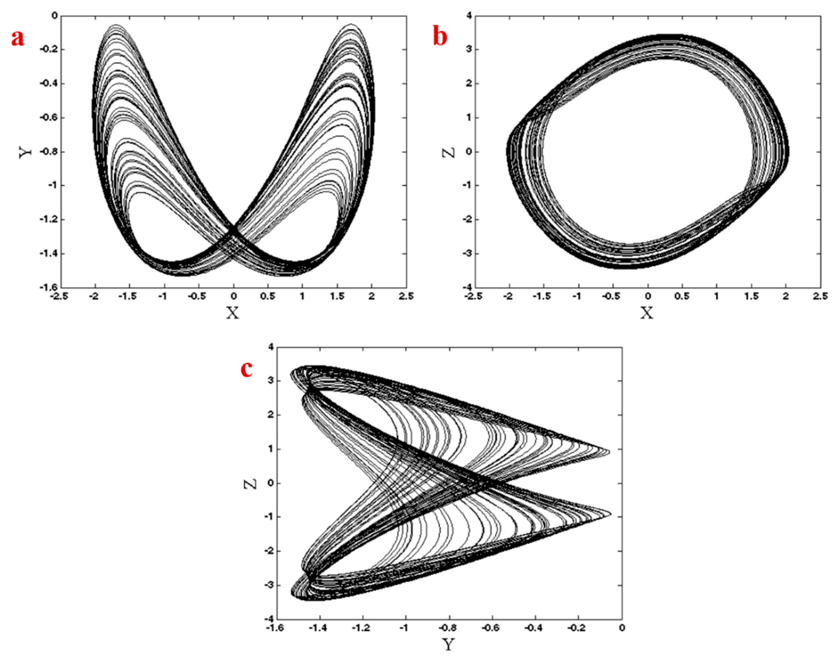
Abstract
1. Introduction
2. The New Chaotic System and Its Structural Properties
3. Dynamical Properties of the Proposed System
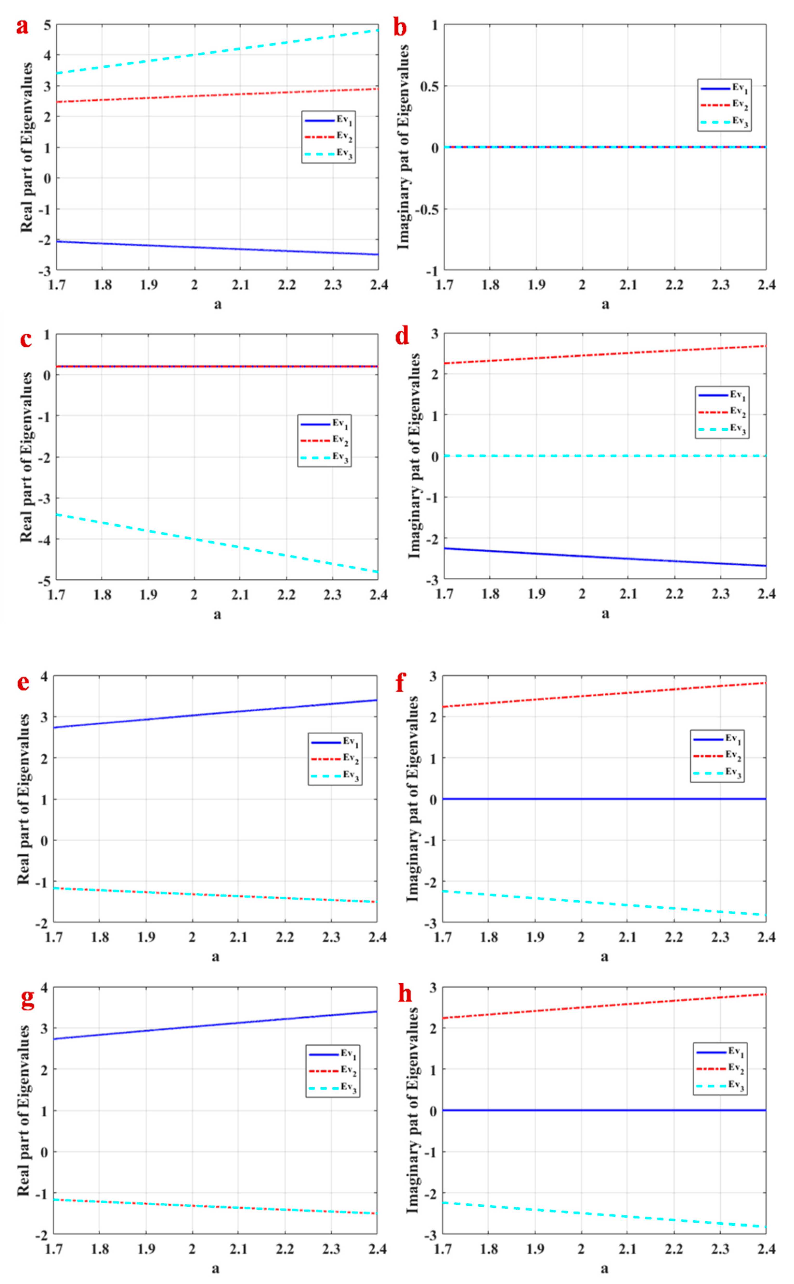
3.1. Equilibrium Points and Their Stability
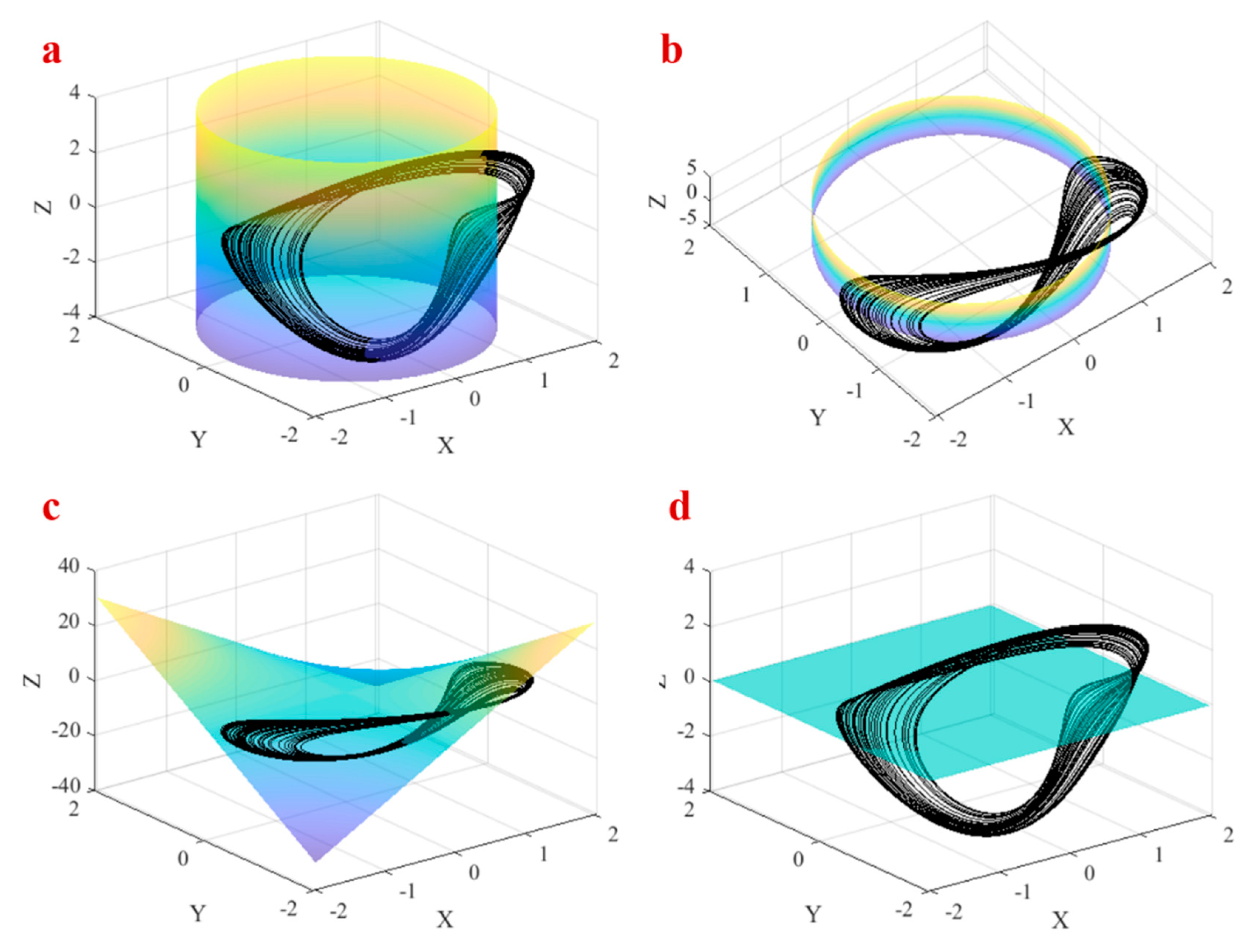
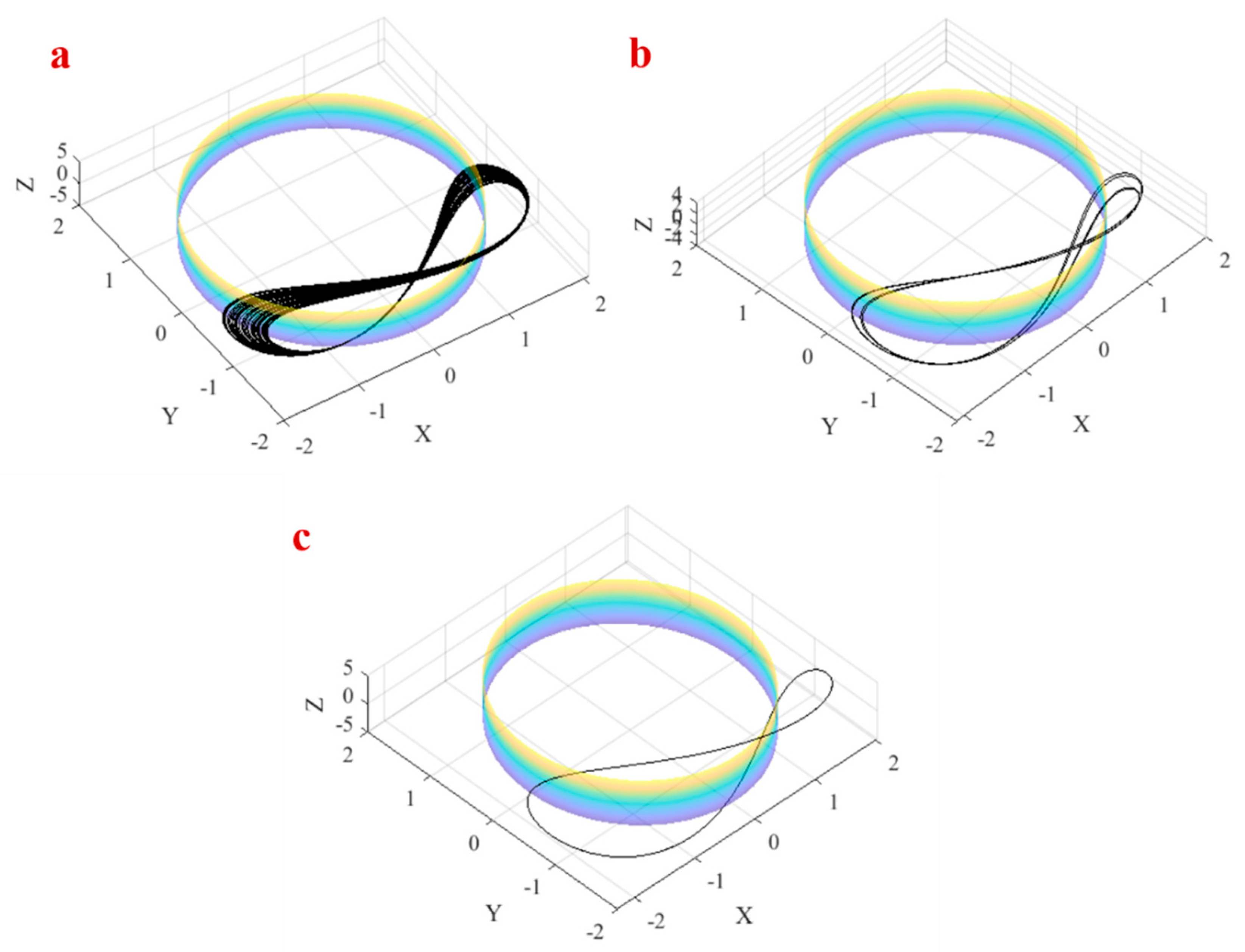
3.2. Attractor around a Pre-Defined Cylinder
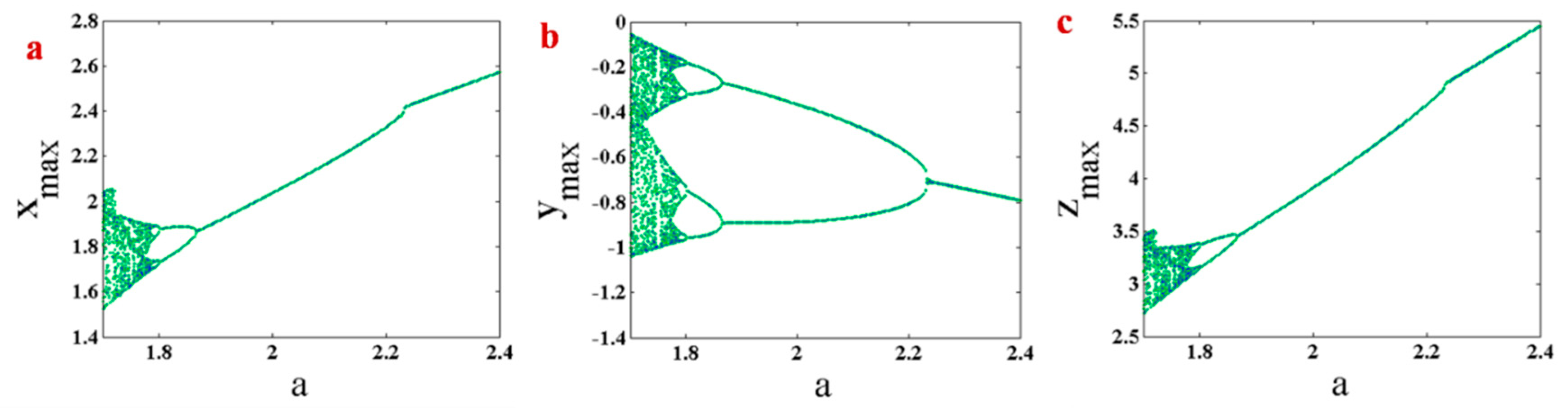
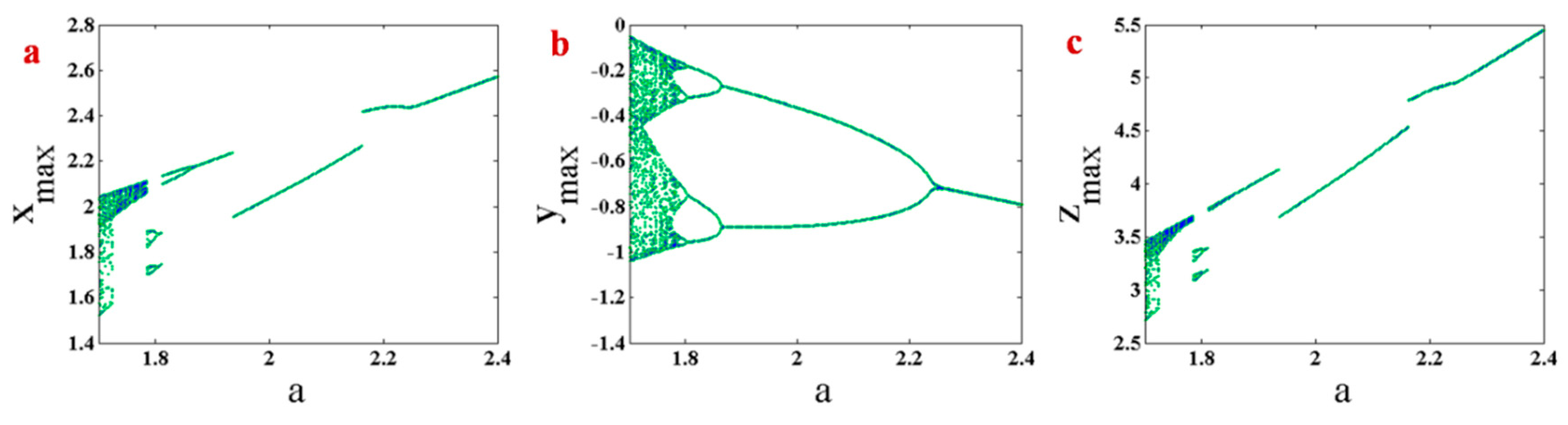
3.3. Bifurcation Diagram
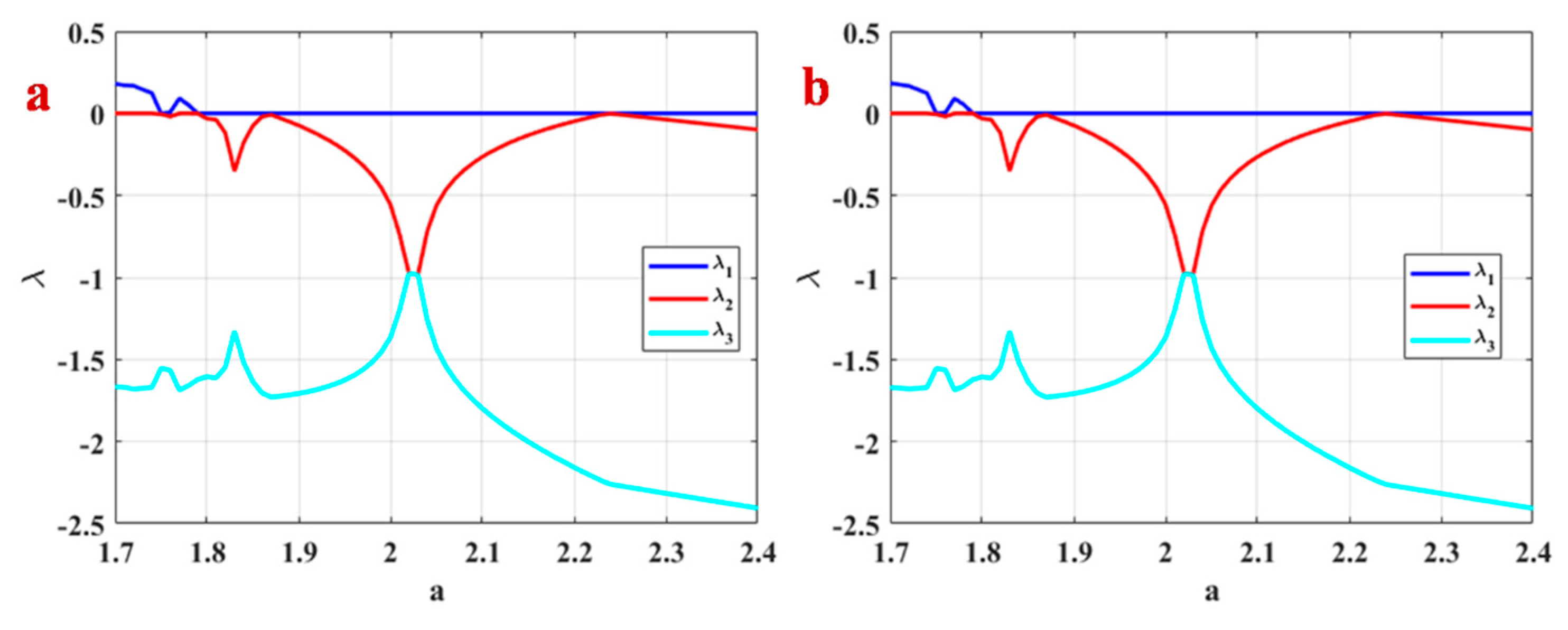
3.4. Lyapunov Exponents
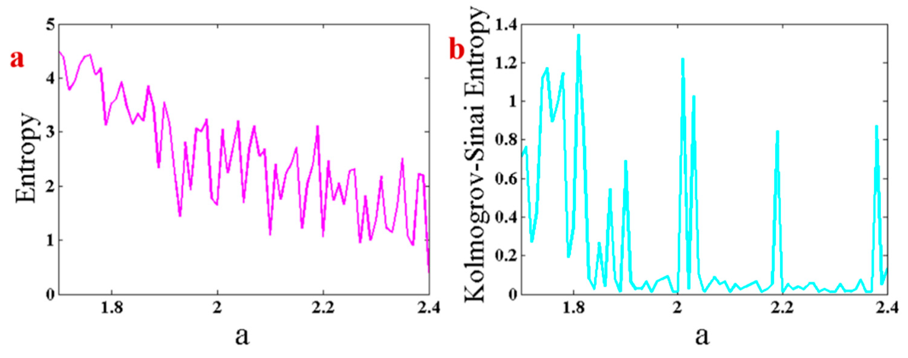
3.5. Entropy Analysis
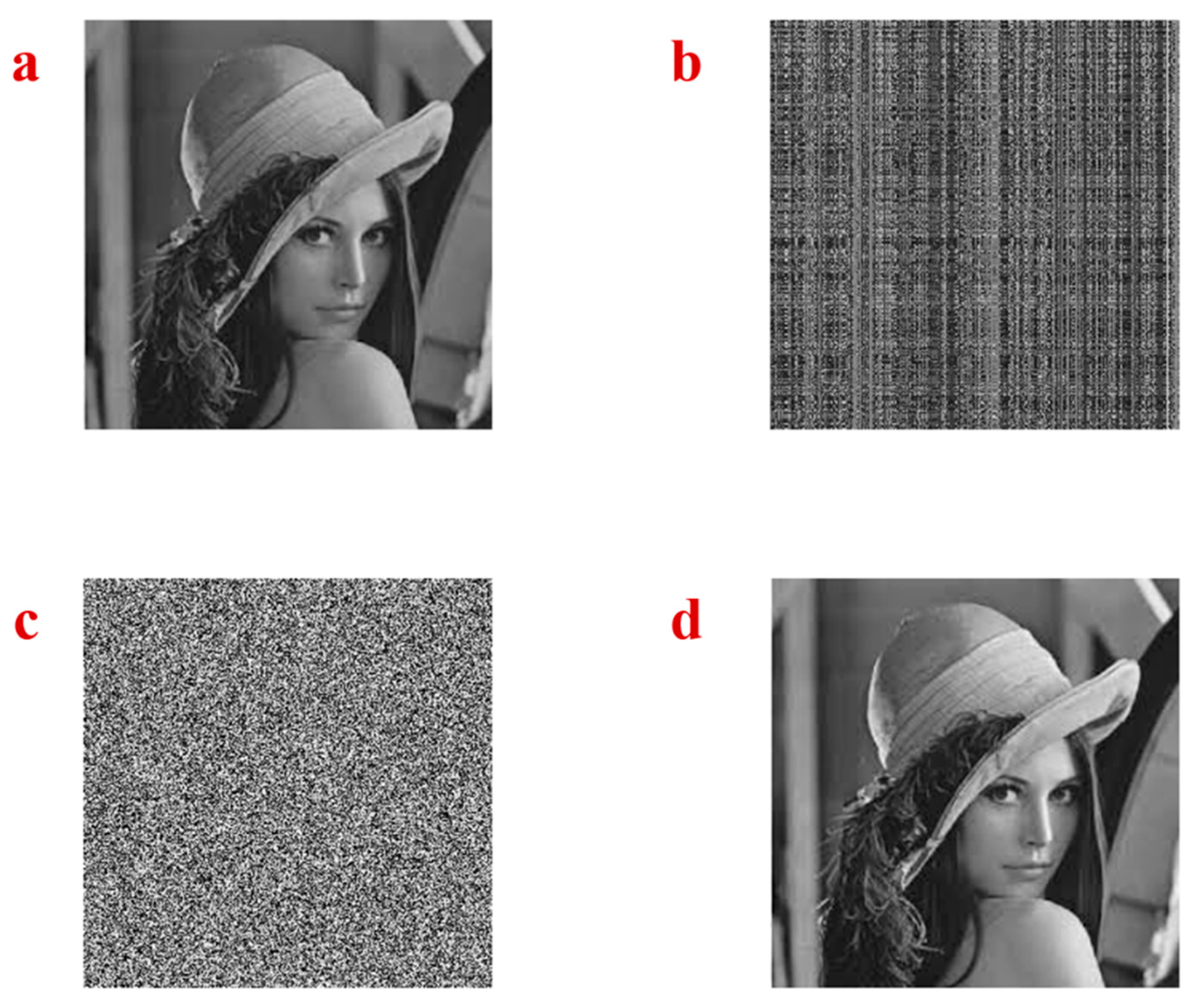
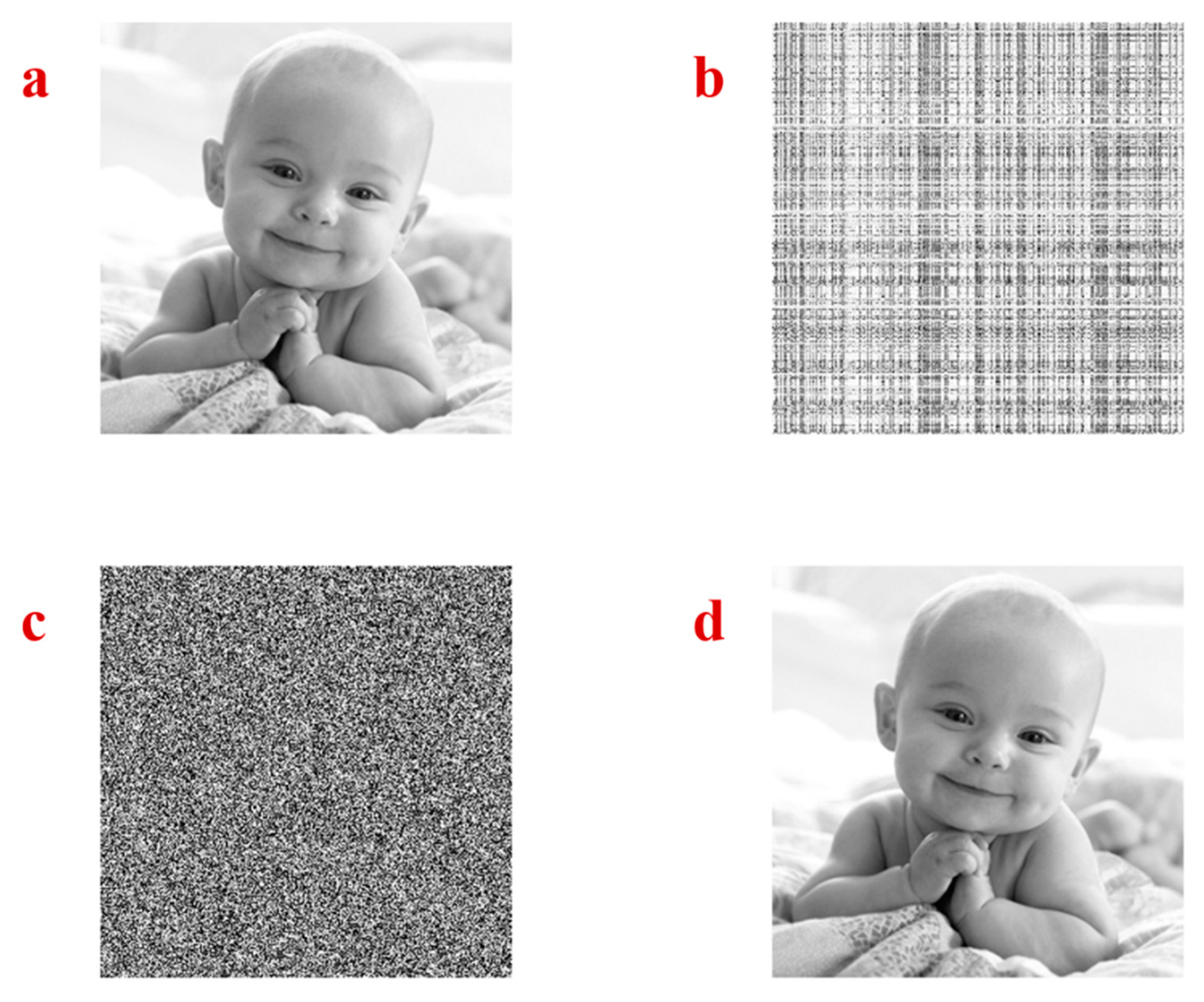
4. Image Encryption
4.1. Encryption Method
| Algorithm 1 Encryption Algorithm |
| 1. Parameter and initial conditions are entered into the system. |
| 2. The proper run time’s step is selected. |
| 3. The float values of the time series are transferred to 32-bit binary values with 3 bits for the integer part and 29 bits for the fraction part. |
| 4. The 20 least significant bits are selected to be used in the generation of random numbers, and they are put in a vector. |
| 5. The rows and columns are shuffled using the randomly generated indices from and variable of chaotic attractor. |
| 6. The random vectors generated by and of chaotic attractor are XORed, and then they are XORed with the shuffled image. |
| 7. The results are converted to decimal. |
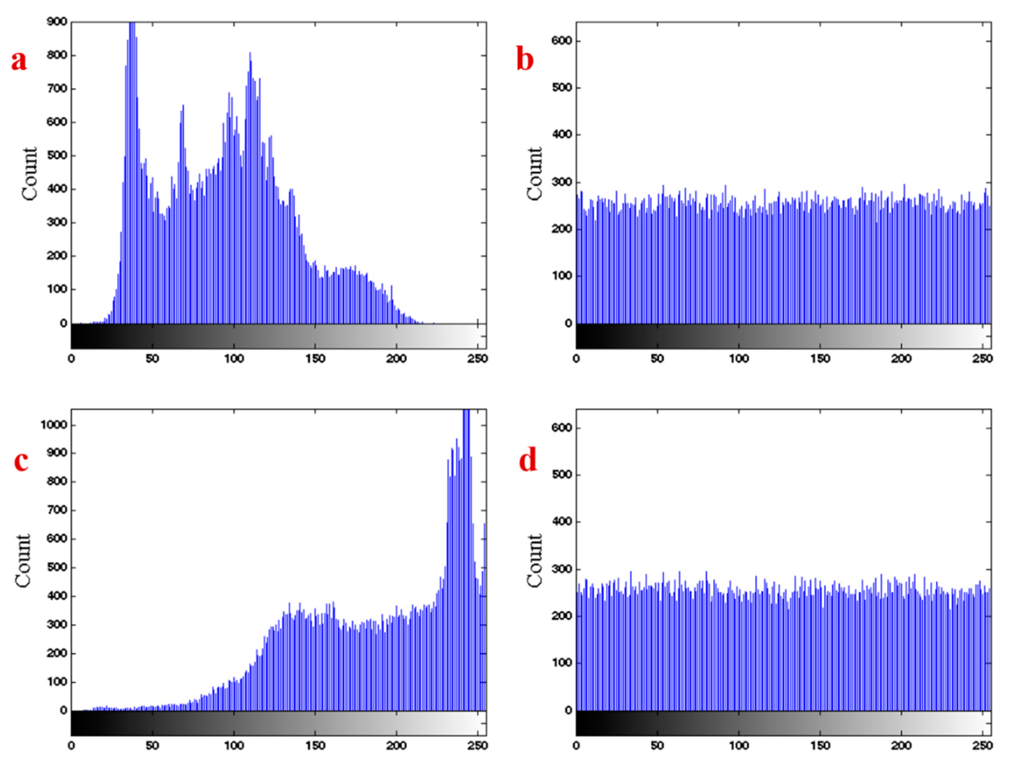
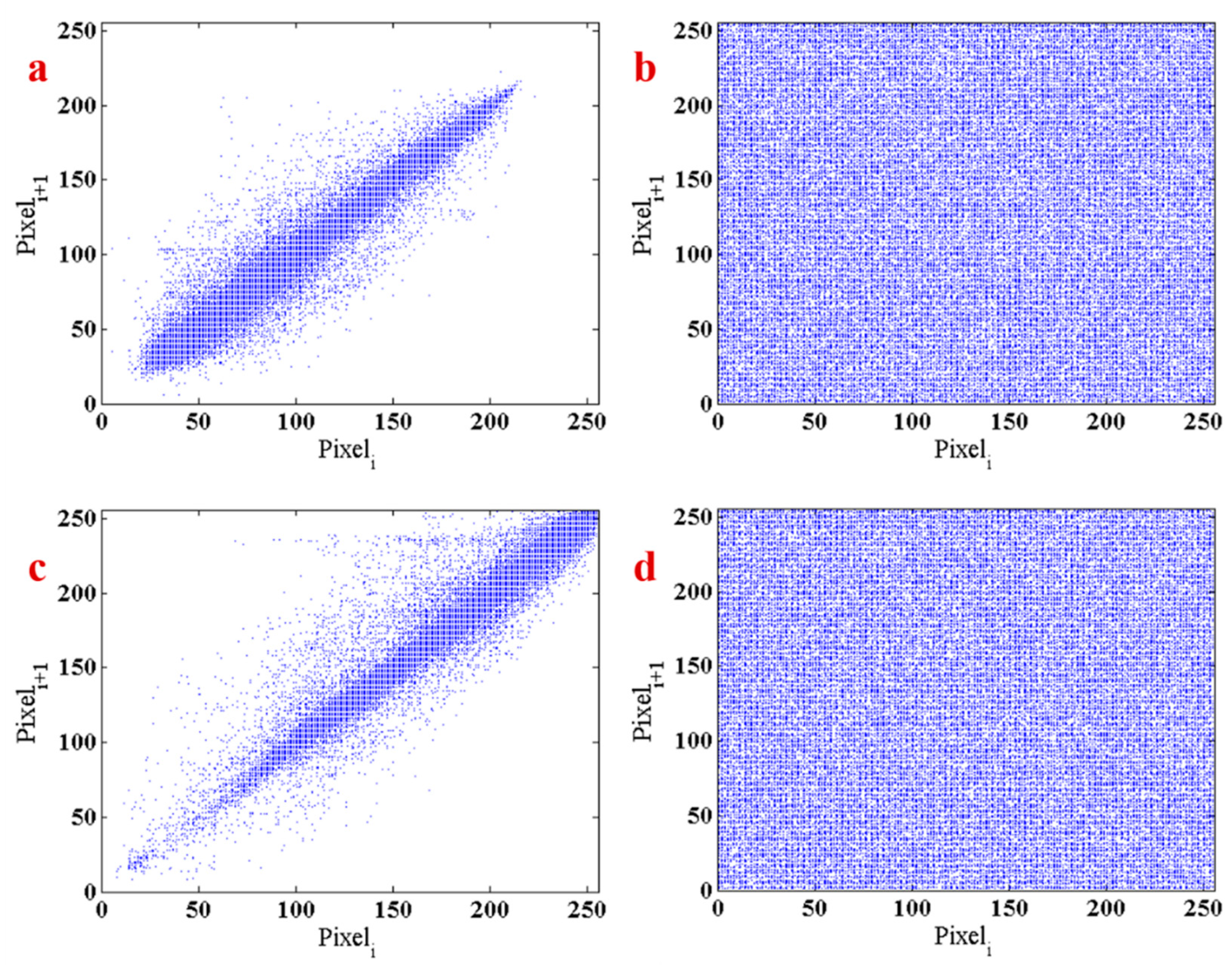
4.2. Encryption’s Performance
5. Conclusions
Author Contributions
Funding
Conflicts of Interest
References
- Danca, M.F.; Tang, W.K.; Chen, G. Suppressing chaos in a simplest autonomous memristor-based circuit of fractional order by periodic impulses. Chaos Solitons Fractals 2016, 84, 31–40. [Google Scholar] [CrossRef]
- Rajagopal, K.; Kacar, S.; Wei, Z.; Duraisamy, P.; Kifle, T.; Karthikeyan, A.; Wei, Z. Dynamical investigation and chaotic associated behaviors of memristor Chua’s circuit with a non-ideal voltage-controlled memristor and its application to voice encryption. AEU Int. J. Electron. Commun. 2019, 107, 183–191. [Google Scholar] [CrossRef]
- Petržela, J.; Kolka, Z.; Hanus, S. Simple chaotic oscillator: From mathematical model to practical experiment. Radioengineering 2006, 15, 6–11. [Google Scholar]
- Chen, G.; Ueta, T. Yet another chaotic attractor. Int. J. Bifurc. Chaos 1999, 9, 1465–1466. [Google Scholar] [CrossRef]
- Lorenz, E.N. Deterministic nonperiodic flow. J. Atmos. Sci. 1963, 20, 130–141. [Google Scholar] [CrossRef]
- Wei, Z. Dynamical behaviors of a chaotic system with no equilibria. Phys. Lett. A 2011, 376, 102–108. [Google Scholar] [CrossRef]
- Wang, X.; Chen, G. A chaotic system with only one stable equilibrium. Commun. Nonlinear Sci. Numer. Simul. 2012, 17, 1264–1272. [Google Scholar] [CrossRef]
- Molaie, M.; Jafari, S.; Sprott, J.C.; Golpayegani, S.M.R.H. Simple chaotic flows with one stable equilibrium. Int. J. Bifurc. Chaos 2013, 23, 1350188. [Google Scholar] [CrossRef]
- Pham, V.T.; Volos, C.; Gambuzza, L.V. A Memristive Hyperchaotic System without Equilibrium. Sci. World J. 2014, 2014, 1–9. [Google Scholar] [CrossRef]
- Pham, V.-T.; Volos, C.; Jafari, S.; Wei, Z.; Wang, X. Constructing a Novel No-Equilibrium Chaotic System. Int. J. Bifurc. Chaos 2014, 24, 1450073. [Google Scholar] [CrossRef]
- Gotthans, T.; Petržela, J. New class of chaotic systems with circular equilibrium. Nonlinear Dyn. 2015, 81, 1143–1149. [Google Scholar] [CrossRef]
- Gotthans, T.; Sprott, J.C.; Petrzela, J. Simple Chaotic Flow with Circle and Square Equilibrium. Int. J. Bifurc. Chaos 2016, 26, 1650137. [Google Scholar] [CrossRef]
- Natiq, H.; Said, M.R.M.; Al-Saidi, N.M.G.; Kilicman, A. Dynamics and Complexity of a New 4D Chaotic Laser System. Entropy 2019, 21, 34. [Google Scholar] [CrossRef]
- Wei, Z.; Sprott, J.; Chen, H. Elementary quadratic chaotic flows with a single non-hyperbolic equilibrium. Phys. Lett. A 2015, 379, 2184–2187. [Google Scholar] [CrossRef]
- Pham, V.T.; Volos, C.; Jafari, S.; Wang, X. Generating a novel hyperchaotic system out of equilibrium. Optoelectron. Adv. Mater. Rapid Commun. 2014, 8, 535–539. [Google Scholar]
- Lai, Q.; Chen, S. Generating Multiple Chaotic Attractors from Sprott B System. Int. J. Bifurc. Chaos 2016, 26, 1650177. [Google Scholar] [CrossRef]
- Pham, V.T.; Jafari, S.; Volos, C.; Wang, X.; Golpayegani, S.M.R.H. Is that Really Hidden? The Presence of Complex Fixed-Points in Chaotic Flows with No Equilibria. Int. J. Bifurc. Chaos 2014, 24, 1450146. [Google Scholar] [CrossRef]
- Wang, Z.; Sun, W.; Wei, Z.; Xi, X. Dynamics analysis and robust modified function projective synchronization of Sprott E system with quadratic perturbation. Kybernetika 2014, 50, 616–631. [Google Scholar] [CrossRef][Green Version]
- Li, C.; Thio, W.J.C.; Sprott, J.C.; Iu, H.H.C.; Xu, Y.; Iu, H.H.C. Constructing Infinitely Many Attractors in a Programmable Chaotic Circuit. IEEE Access 2018, 6, 29003–29012. [Google Scholar] [CrossRef]
- Ma, J.; Zhou, P.; Ahmad, B.; Ren, G.; Wang, C. Chaos and multi-scroll attractors in RCL-shunted junction coupled Jerk circuit connected by memristor. PLoS ONE 2018, 13, e0191120. [Google Scholar] [CrossRef]
- Wei, Z.; Zhu, B.; Yang, J.; Perc, M.; Slavinec, M. Bifurcation analysis of two disc dynamos with viscous friction and multiple time delays. Appl. Math. Comput. 2019, 347, 265–281. [Google Scholar] [CrossRef]
- Li, C.; Sprott, J.C. An infinite 3-D quasiperiodic lattice of chaotic attractors. Phys. Lett. A 2018, 382, 581–587. [Google Scholar] [CrossRef]
- PETRŽELA, J.; HRUBOŠ, Z.; GOTTHANS, T. Modeling Deterministic Chaos Using Electronic Circuits. Radioengineering 2011, 20, 438–444. [Google Scholar]
- Zhou, P.; Huang, K. A new 4-D non-equilibrium fractional-order chaotic system and its circuit implementation. Commun. Nonlinear Sci. Numer. Simul. 2014, 19, 2005–2011. [Google Scholar] [CrossRef]
- Danca, M.F.; Bourke, P.; Kuznetsov, N. Graphical Structure of Attraction Basins of Hidden Chaotic Attractors: The Rabinovich–Fabrikant System. Int. J. Bifurc. Chaos 2019, 29, 1930001. [Google Scholar] [CrossRef]
- Kuznetsov, N.V.; Leonov, G.A.; Mokaev, T.N. Localization of a hidden attractor in the Rabinovich system. arXiv 2015, arXiv:150404723. [Google Scholar]
- Kuznetsov, N.V.; Leonov, G.A.; Mokaev, T.N.; Seledzhi, S.M. Hidden Attractor in the Rabinovich System, Chua Circuits and PLL. In AIP Conference Proceedings; AIP Publishing: Melville, NY, USA, 2016. [Google Scholar]
- Kuznetsov, N.V.; Leonov, G.A.; Mokaev, T.N. The Lyapunov dimension and its computation for self-excited and hidden attractors in the Glukhovsky-Dolzhansky fluid convection model. arXiv 2015, arXiv:150909161. [Google Scholar]
- Danca, M.-F.; Fečkan, M. Hidden chaotic attractors and chaos suppression in an impulsive discrete economical supply and demand dynamical system. Commun. Nonlinear Sci. Numer. Simul. 2019, 74, 1–13. [Google Scholar] [CrossRef]
- Danca, M.F.; Kuznetsov, N.; Chen, G. Unusual dynamics and hidden attractors of the Rabinovich–Fabrikant system. Nonlinear Dyn. 2017, 88, 791–805. [Google Scholar] [CrossRef]
- Lai, Q.; Akgul, A.; Zhao, X.W.; Pei, H. Various Types of Coexisting Attractors in a New 4D Autonomous Chaotic System. Int. J. Bifurc. Chaos 2017, 27, 1750142. [Google Scholar] [CrossRef]
- Chen, S.; Lai, Q. Coexisting attractors generated from a new 4D smooth chaotic system. Int. J. Control. Autom. Syst. 2016, 14, 1124–1131. [Google Scholar]
- Bao, B.; Jiang, T.; Xu, Q.; Chen, M.; Wu, H.; Hu, Y. Coexisting infinitely many attractors in active band-pass filter-based memristive circuit. Nonlinear Dyn. 2016, 86, 1711–1723. [Google Scholar] [CrossRef]
- Bao, B.C.; Li, Q.D.; Wang, N.; Xu, Q. Multistability in Chua’s circuit with two stable node-foci. Chaos Interdiscip. J. Nonlinear Sci. 2016, 26, 043111. [Google Scholar] [CrossRef] [PubMed]
- Bao, B.C.; Chen, M.; Bao, H.; Xu, Q. Extreme multistability in a memristive circuit. Electron. Lett. 2016, 52, 1008–1010. [Google Scholar] [CrossRef]
- Danca, M.-F. Lyapunov Exponents of a Discontinuous 4D Hyperchaotic System of Integer or Fractional Order. Entropy 2018, 20, 337. [Google Scholar] [CrossRef]
- Sprott, J.C. Elegant Chaos: Algebraically Simple Chaotic Flows; World Scientific: Singapore, 2010. [Google Scholar]
- Hilborn, R.C. Chaos and Nonlinear Dynamics: An Introduction for Scientists and Engineers; Oxford University Press: Oxford, UK, 2000. [Google Scholar]
- He, S.; Sun, K.; Wang, R. Fractional fuzzy entropy algorithm and the complexity analysis for nonlinear time series. Eur. Phys. J. Spec. Top. 2018, 227, 943–957. [Google Scholar] [CrossRef]
- He, S.-B.; Sun, K.-H.; Zhu, C.X. Complexity analyses of multi-wing chaotic systems. Chin. Phys. B 2013, 22, 050506. [Google Scholar] [CrossRef]
- He, S.; Sun, K.; Wang, H. Complexity Analysis and DSP Implementation of the Fractional-Order Lorenz Hyperchaotic System. Entropy 2015, 17, 8299–8311. [Google Scholar] [CrossRef]
- He, S.; Li, C.; Sun, K.; Jafari, S. Multivariate Multiscale Complexity Analysis of Self-Reproducing Chaotic Systems. Entropy 2018, 20, 556. [Google Scholar] [CrossRef]
- Hržić, F.; Štajduhar, I.; Tschauner, S.; Sorantin, E.; Lerga, J. Local-Entropy Based Approach for X-Ray Image Segmentation and Fracture Detection. Entropy 2019, 21, 338. [Google Scholar] [CrossRef]
- Bourbakis, N.; Alexopoulos, C. Picture data encryption using scan patterns. Pattern Recognit. 1992, 25, 567–581. [Google Scholar] [CrossRef]
- Pareek, N.; Patidar, V.; Sud, K. Image encryption using chaotic logistic map. Image Vis. Comput. 2006, 24, 926–934. [Google Scholar] [CrossRef]
- Natiq, H.; Al-Saidi, N.M.G.; Said, M.R.M.; Kilicman, A. A new hyperchaotic map and its application for image encryption. Eur. Phys. J. Plus 2018, 133, 6. [Google Scholar] [CrossRef]
- Nazarimehr, F.; Jafari, S.; Golpayegani, S.M.R.H.; Perc, M.; Sprott, J.C. Predicting tipping points of dynamical systems during a period-doubling route to chaos. Chaos Interdiscip. J. Nonlinear Sci. 2018, 28, 073102. [Google Scholar] [CrossRef]
- Nazarimehr, F.; Ghaffari, A.; Jafari, S.; Golpayegani, S.M.R.H. Sparse Recovery and Dictionary Learning to Identify the Nonlinear Dynamical Systems: One Step Toward Finding Bifurcation Points in Real Systems. Int. J. Bifurc. Chaos 2019, 29, 1950030. [Google Scholar] [CrossRef]
- Beritelli, F.; Di Cola, E.; Fortuna, L.; Italia, F. Multilayer Chaotic Encryption for Secure Communications in Packet Switching Networks. In Proceedings of the International Conference on Communication Technology Proceedings, Beijing, China, 21–25 August 2000. [Google Scholar]
- Gunay, S.; Kaşkaloğlu, K. Seeking a Chaotic Order in the Cryptocurrency Market. Math. Comput. Appl. 2019, 24, 36. [Google Scholar] [CrossRef]
- Álvarez, G.; Li, S. Some basic cryptographic requirements for chaos-based cryptosystems. Int. J. Bifurc. Chaos 2006, 16, 2129–2151. [Google Scholar] [CrossRef]
- Wang, J.; Ding, Q. Dynamic Rounds Chaotic Block Cipher Based on Keyword Abstract Extraction. Entropy 2018, 20, 693. [Google Scholar] [CrossRef]
- Çavuşoğlu, Ü; Kaçar, S.; Pehlivan, I.; Zengin, A. Secure image encryption algorithm design using a novel chaos based S-Box. Chaos Solitons Fractals 2017, 95, 92–101. [Google Scholar]
- Lagmiri, S.; Elalami, N.; Elalami, J. Novel Chaotic System for Color Image Encryption Using Random Permutation. Int. J. Comput. Netw. Commun. Secur. 2018, 6, 9–16. [Google Scholar]
- Çavuşoğlu, Ü.; Panahi, S.; Akgül, A.; Jafari, S.; Kaçar, S. A new chaotic system with hidden attractor and its engineering applications: Analog circuit realization and image encryption. Analog Integr. Circuits Signal Process. 2019, 98, 85–99. [Google Scholar] [CrossRef]
- Abdallah, E.E.; Ben Hamza, A.; Bhattacharya, P. MPEG Video Watermarking Using Tensor Singular Value Decomposition. In Proceedings of the Computer Vision–ECCV 2012, Florence, Italy, 7–13 October 2012; Springer: Berlin/Heidelberg, Germany, 2017. [Google Scholar]
- Abdallah, E.E.; Hamza, A.B.; Bhattacharya, P. Video watermarking using wavelet transform and tensor algebra. Signal Image Video Process. 2010, 4, 233–245. [Google Scholar] [CrossRef]
- Ouhsain, M.; Ben Hamza, A. Image watermarking scheme using nonnegative matrix factorization and wavelet transform. Expert Syst. Appl. 2009, 36, 2123–2129. [Google Scholar] [CrossRef]
- Jafari, S.; Sprott, J.C.; Dehghan, S. Categories of conservative flows. Int. J. Bifurc. Chaos 2019, 29, 1950021. [Google Scholar] [CrossRef]
- Wolf, A.; Swift, J.B.; Swinney, H.L.; Vastano, J.A. Determining Lyapunov exponents from a time series. Phys. D Nonlinear Phenom. 1985, 16, 285–317. [Google Scholar] [CrossRef]
- Lerga, J.; Saulig, N.; Mozetič, V. Algorithm based on the short-term Rényi entropy and IF estimation for noisy EEG signals analysis. Comput. Biol. Med. 2017, 80, 1–13. [Google Scholar] [CrossRef]
- Lerga, J.; Saulig, N.; Mozetic, V.; Lerga, R. Number of EEG Signal Components estimated Using the Short-Term Rényi Entropy. In Proceedings of the International Multidisciplinary Conference on Computer and Energy Science (SpliTech), Split, Croatia, 13–15 July 2016. [Google Scholar]
- Cover, T.M.; Thomas, J.A. Elements of Information Theory; John Wiley & Sons: Hoboken, NJ, USA, 2012. [Google Scholar]
- Frigg, R. In What Sense is the Kolmogorov-Sinai Entropy a Measure for Chaotic Behaviour?--Bridging the Gap Between Dynamical Systems Theory and Communication Theory. Br. J. Philos. Sci. 2004, 55, 411–434. [Google Scholar] [CrossRef]
- Mihelich, M.; Dubrulle, B.; Paillard, D.; Herbert, C. Maximum Entropy Production vs. Kolmogorov-Sinai Entropy in a Constrained ASEP Model. Entropy 2014, 16, 1037–1046. [Google Scholar] [CrossRef]
- Jolfaei, A.; Mirghadri, A. A new approach to measure quality of image encryption. Int. J. Comput. Netw. Secur. 2010, 2, 38–44. [Google Scholar]


© 2019 by the authors. Licensee MDPI, Basel, Switzerland. This article is an open access article distributed under the terms and conditions of the Creative Commons Attribution (CC BY) license (http://creativecommons.org/licenses/by/4.0/).
Share and Cite
Farhan, A.K.; Al-Saidi, N.M.G.; Maolood, A.T.; Nazarimehr, F.; Hussain, I. Entropy Analysis and Image Encryption Application Based on a New Chaotic System Crossing a Cylinder. Entropy 2019, 21, 958. https://doi.org/10.3390/e21100958
Farhan AK, Al-Saidi NMG, Maolood AT, Nazarimehr F, Hussain I. Entropy Analysis and Image Encryption Application Based on a New Chaotic System Crossing a Cylinder. Entropy. 2019; 21(10):958. https://doi.org/10.3390/e21100958
Chicago/Turabian StyleFarhan, Alaa Kadhim, Nadia M.G. Al-Saidi, Abeer Tariq Maolood, Fahimeh Nazarimehr, and Iqtadar Hussain. 2019. "Entropy Analysis and Image Encryption Application Based on a New Chaotic System Crossing a Cylinder" Entropy 21, no. 10: 958. https://doi.org/10.3390/e21100958
APA StyleFarhan, A. K., Al-Saidi, N. M. G., Maolood, A. T., Nazarimehr, F., & Hussain, I. (2019). Entropy Analysis and Image Encryption Application Based on a New Chaotic System Crossing a Cylinder. Entropy, 21(10), 958. https://doi.org/10.3390/e21100958