On Data-Processing and Majorization Inequalities for f-Divergences with Applications

Abstract

This paper is focused on the derivation of data-processing and majorization inequalities for f-divergences, and their applications in information theory and statistics. For the accessibility of the material, the main results are first introduced without proofs, followed by exemplifications of the theorems with further related analytical results, interpretations, and information-theoretic applications. One application refers to the performance analysis of list decoding with either fixed or variable list sizes; some earlier bounds on the list decoding error probability are reproduced in a unified way, and new bounds are obtained and exemplified numerically. Another application is related to a study of the quality of approximating a probability mass function, induced by the leaves of a Tunstall tree, by an equiprobable distribution. The compression rates of finite-length Tunstall codes are further analyzed for asserting their closeness to the Shannon entropy of a memoryless and stationary discrete source. Almost all the analysis is relegated to the appendices, which form the major part of this manuscript.

1. Introduction

Divergences are non-negative measures of dissimilarity between pairs of probability measures which are defined on the same measurable space. They play a key role in the development of information theory, probability theory, statistics, learning, signal processing, and other related fields. One important class of divergence measures is defined by means of convex functions f, and it is called the class of f-divergences. It unifies fundamental and independently-introduced concepts in several branches of mathematics such as the chi-squared test for the goodness of fit in statistics, the total variation distance in functional analysis, the relative entropy in information theory and statistics, and it is closely related to the Rényi divergence which generalizes the relative entropy. The class of f-divergences was introduced in the sixties by Ali and Silvey [1], Csiszár [2,3,4,5,6], and Morimoto [7]. This class satisfies pleasing features such as the data-processing inequality, convexity, continuity and duality properties, finding interesting applications in information theory and statistics (see, e.g., [4,6,8,9,10,11,12,13,14,15]).

This manuscript is a research paper which is focused on the derivation of data-processing and majorization inequalities for f-divergences, and a study of some of their potential applications in information theory and statistics. Preliminaries are next provided.

1.1. Preliminaries and Related Works

We provide here definitions and known results from the literature which serve as a background to the presentation in this paper. We first provide a definition for the family of f-divergences.

Definition 1

([16], p. 4398). Let P and Q be probability measures, let μ be a dominating measure of P and Q (i.e., $P,Q\ll \mu$), and let $p:=\frac{dP}{d\mu }$ and $q:=\frac{dQ}{d\mu }$. The f-divergence from P to Q is given, independently of μ, by

$$\begin{array}{c}\hfill D_f(P\parallel Q):=\int qf\left(\frac{p}{q}\right)d\mu ,\end{array}$$

(1)

where

$$f\left(0\right):={\displaystyle \underset{t\to 0^{+}}{lim}}f\left(t\right),$$

(2)

$$0f\left(\frac{0}{0}\right):=0,$$

(3)

$$0f\left(\frac{a}{0}\right):={\displaystyle \underset{t\to 0^{+}}{lim}}tf\left(\frac{a}{t}\right)=a{\displaystyle \underset{u\to \infty }{lim}}\frac{f\left(u\right)}{u},a>0.$$

(4)

Definition 2.

Let $Q_X$ be a probability distribution which is defined on a set $\mathcal{X}$, and that is not a point mass, and let $W_{Y|X}:\mathcal{X}\to \mathcal{Y}$ be a stochastic transformation. The contraction coefficient for f-divergences is defined as

$$\begin{array}{c}\hfill {\mu }_f(Q_X,W_{Y|X}):={\displaystyle \underset{P_X:D_f(P_X\parallel Q_X)\in (0,\infty )}{sup}}\frac{D_f(P_Y\parallel Q_Y)}{D_f(P_X\parallel Q_X)},\end{array}$$

(5)

where, for all $y\in \mathcal{Y}$,

$$P_Y\left(y\right)=\left(P_X{W}_{Y|X}\right)\left(y\right):={\int }_{\mathcal{X}}\mathrm{d}{P}_X\left(x\right)W_{Y|X}\left(y\right|x),$$

(6)

$$Q_Y\left(y\right)=\left(Q_X{W}_{Y|X}\right)\left(y\right):={\int }_{\mathcal{X}}\mathrm{d}{Q}_X\left(x\right)W_{Y|X}\left(y\right|x).$$

(7)

The notation in (6) and (7), and also in (20), (21), (42), (43), (44) in the continuation of this paper, is consistent with the standard notation used in information theory (see, e.g., the first displayed equation after (3.2) in [17]).

Contraction coefficients for f-divergences play a key role in strong data-processing inequalities (see [18,19,20], ([21], Chapter II), [22,23,24,25,26]). The following are essential definitions and results which are related to maximal correlation and strong data-processing inequalities.

Definition 3.

The maximal correlation between two random variables X and Y is defined as

$$\begin{array}{c}\hfill {\rho }_{\mathrm{m}}(X;Y):={\displaystyle \underset{f,g}{sup}}\mathbb{E}\left[f\left(X\right)g\left(Y\right)\right],\end{array}$$

(8)

where the supremum is taken over all real-valued functions f and g such that

$$\begin{array}{c}\hfill \mathbb{E}\left[f\left(X\right)\right]=\mathbb{E}\left[g\left(Y\right)\right]=0,\mathbb{E}\left[f^2\left(X\right)\right]\le 1,\mathbb{E}\left[g^2\left(Y\right)\right]\le 1.\end{array}$$

(9)

Definition 4.

Pearson’s ${\chi }^2$-divergence [27] from P to Q is defined to be the f-divergence from P to Q (see Definition 1) with $f\left(t\right)={(t-1)}^2$ or $f\left(t\right)=t^2-1$ for all $t>0$,

$$\begin{array}{cc}\hfill {\chi }^2(P\parallel Q)& :=D_f(P\parallel Q)\hfill \end{array}$$

(10)

$$\begin{array}{cc}& =\int \frac{{(p-q)}^2}{q}d\mu \hfill \end{array}$$

(11)

$$\begin{array}{cc}& =\int \frac{p^2}{q}d\mu -1\hfill \end{array}$$

(12)

independently of the dominating measure μ (i.e., $P,Q\ll \mu$, e.g., $\mu =P+Q$).

Neyman’s ${\chi }^2$-divergence [28] from P to Q is the Pearson’s ${\chi }^2$-divergence from Q to P, i.e., it is equal to

$$\begin{array}{c}\hfill {\chi }^2(Q\parallel P)=D_g(P\parallel Q)\end{array}$$

(13)

with $g\left(t\right)=\frac{{(t-1)}^2}{t}$ or $g\left(t\right)=\frac{1}{t}-t$ for all $t>0$.

Proposition 1

(([24], Theorem 3.2), [29]). The contraction coefficient for the ${\chi }^2$-divergence satisfies

$$\begin{array}{c}\hfill {\mu }_{{\chi }^2}(Q_X,W_{Y|X})={\rho }_{\mathrm{m}}^2(X;Y)\end{array}$$

(14)

with $X\sim Q_X$ and $Y\sim Q_Y$ (see (7)).

Proposition 2

([25], Theorem 2). Let $f:(0,\infty )\to \mathbb{R}$ be convex and twice continuously differentiable with $f\left(1\right)=0$ and $f^{″}\left(1\right)>0$. Then, for any $Q_X$ that is not a point mass,

$$\begin{array}{c}\hfill {\mu }_{{\chi }^2}(Q_X,W_{Y|X})\le {\mu }_f(Q_X,W_{Y|X}),\end{array}$$

(15)

i.e., the contraction coefficient for the ${\chi }^2$-divergence is the minimal contraction coefficient among all f-divergences with f satisfying the above conditions.

Remark 1.

A weaker version of (15) was presented in ([21], Proposition II.6.15) in the general alphabet setting, and the result in (15) was obtained in ([24], Theorem 3.3) for finite alphabets.

The following result provides an upper bound on the contraction coefficient for a subclass of f-divergences in the finite alphabet setting.

Proposition 3

([26], Theorem 8). Let $f:[0,\infty )\to \mathbb{R}$ be a continuous convex function which is three times differentiable at unity with $f\left(1\right)=0$ and $f^{″}\left(1\right)>0$, and let it further satisfy the following conditions:

(a) 

$$\begin{array}{c}\hfill \left(f\left(t\right)-f^{\prime }\left(1\right)(t-1)\right)\left(1-\frac{f^{\left(3\right)}\left(1\right)(t-1)}{3f^{″}\left(1\right)}\right)\ge \frac{1}{2}{f}^{″}\left(1\right){(t-1)}^2,\forall t>0.\end{array}$$

(16)

(b) 

The function $g:(0,\infty )\to \mathbb{R}$, given by $g\left(t\right):=\frac{f\left(t\right)-f\left(0\right)}{t}$ for all $t>0$, is concave.

Then, for a probability mass function $Q_X$ supported over a finite set $\mathcal{X}$,

$$\begin{array}{c}\hfill {\mu }_f(Q_X,W_{Y|X})\le \left(\frac{f^{\prime }\left(1\right)+f\left(0\right)}{f^{″}\left(1\right){\displaystyle \underset{x\in \mathcal{X}}{min}}{Q}_X\left(x\right)}\right){\mu }_{{\chi }^2}(Q_X,W_{Y|X}).\end{array}$$

(17)

For the presentation of our majorization inequalities for f-divergences and related entropy bounds (see Section 2.3), essential definitions and basic results are next provided (see, e.g., [30], ([31], Chapter 13) and ([32], Chapter 2)). Let P be a probability mass function defined on a finite set $\mathcal{X}$, let $p_{max}$ be the maximal mass of P, and let $G_P\left(k\right)$ be the sum of the k largest masses of P for $k\in \{1,\dots ,|\mathcal{X}\left|\right\}$ (hence, it follows that $G_P\left(1\right)=p_{max}$ and $G_P\left(\right|\mathcal{X}\left|\right)=1$).

Definition 5.

Consider discrete probability mass functions P and Q defined on a finite set $\mathcal{X}$. It is said that P is majorized by Q (or Q majorizes P), and it is denoted by $P\prec Q$, if $G_P\left(k\right)\le G_Q\left(k\right)$ for all $k\in \{1,\dots ,|\mathcal{X}\left|\right\}$ (recall that $G_P\left(\right|\mathcal{X}\left|\right)=G_Q\left(\right|\mathcal{X}\left|\right)=1$).

A unit mass majorizes any other distribution; on the other hand, the equiprobable distribution on a finite set is majorized by any other distribution defined on the same set.

Definition 6.

Let ${\mathcal{P}}_n$ denote the set of all the probability mass functions that are defined on ${\mathcal{A}}_n:=\{1,\dots ,n\}$. A function $f:{\mathcal{P}}_n\to \mathbb{R}$ is said to be Schur-convex if for every $P,Q\in {\mathcal{P}}_n$ such that $P\prec Q$, we have $f\left(P\right)\le f\left(Q\right)$. Likewise, f is said to be Schur-concave if $-f$ is Schur-convex, i.e., $P,Q\in {\mathcal{P}}_n$ and $P\prec Q$ imply that $f\left(P\right)\ge f\left(Q\right)$.

Characterization of Schur-convex functions is provided, e.g., in ([30], Chapter 3). For example, there exist some connections between convexity and Schur-convexity (see, e.g., ([30], Section 3.C) and ([32], Chapter 2.3)). However, a Schur-convex function is not necessarily convex ([32], Example 2.3.15).

Finally, what is the connection between data processing and majorization, and why these types of inequalities are both considered in the same manuscript? This connection is provided in the following fundamental well-known result (see, e.g., ([32], Theorem 2.1.10), ([30], Theorem B.2) and ([31], Chapter 13)):

Proposition 4.

Let P and Q be probability mass functions defined on a finite set $\mathcal{A}$. Then, $P\prec Q$ if and only if there exists a doubly-stochastic transformation $W_{Y|X}:\mathcal{A}\to \mathcal{A}$ (i.e., ${\displaystyle \sum _{x\in \mathcal{A}}}{W}_{Y|X}\left(y\right|x)=1$ for all $y\in \mathcal{A}$, and ${\displaystyle \sum _{y\in \mathcal{A}}}{W}_{Y|X}\left(y\right|x)=1$ for all $x\in \mathcal{A}$ with $W_{Y|X}(·|·)\ge 0$) such that $Q\to W_{Y|X}\to P$. In other words, $P\prec Q$ if and only if in their representation as column vectors, there exists a doubly-stochastic matrix $\mathbf{W}$ (i.e., a square matrix with non-negative entries such that the sum of each column or each row in $\mathbf{W}$ is equal to 1) such that $P=\mathbf{W}Q$.

1.2. Contributions

This paper is focused on the derivation of data-processing and majorization inequalities for f-divergences, and it applies these inequalities to information theory and statistics.

The starting point for obtaining strong data-processing inequalities in this paper relies on the derivation of lower and upper bounds on the difference $D_f(P_X\parallel Q_X)-D_f(P_Y\parallel Q_Y)$ where $(P_X,Q_X)$ and $(P_Y,Q_Y)$ denote, respectively, pairs of input and output probability distributions with a given stochastic transformation $W_{Y|X}$ (i.e., where $P_X\to W_{Y|X}\to P_Y$ and $Q_X\to W_{Y|X}\to Q_Y$). These bounds are expressed in terms of the respective difference in the Pearson’s or Neyman’s ${\chi }^2$-divergence, and they hold for all f-divergences (see Theorems 1 and 2). By a different approach, we derive an upper bound on the contraction coefficient for f-divergences of a certain type, which gives an alternative strong data-processing inequality for the considered type of f-divergences (see Theorems 3 and 4). In this framework, a parametric subclass of f-divergences is introduced, its interesting properties are studied (see Theorem 5), all the data-processing inequalities which are derived in this paper are applied to this subclass, and these inequalities are exemplified numerically to examine their tightness (see Section 3.1).

This paper also derives majorization inequalities for f-divergences where part of these inequalities rely on the earlier data-processing inequalities (see Theorem 6). A different approach, which relies on the concept of majorization, serves to derive tight bounds on the maximal value of an f-divergence from a probability mass function P to an equiprobable distribution; the maximization is carried over all P with a fixed finite support where the ratio of their maximal to minimal probability masses does not exceed a given value (see Theorem 7). These bounds lead to accurate asymptotic results which apply to general f-divergences, and they strengthen and generalize recent results of this type with respect to the relative entropy [33], and the Rényi divergence [34]. Furthermore, we explore in Theorem 7 the convergence rates to the asymptotic results. Data-processing and majorization inequalities also serve to strengthen the Schur-concavity property of the Tsallis entropy (see Theorem 8), showing by a comparison to earlier bounds in [35,36] that none of these bounds is superseded by the other. Further analytical results which are related to the specialization of our central result on majorization inequalities in Theorem 7, applied to several important sub-classes of f-divergences, are provided in Section 3.2 (including Theorem 9). A quantity which is involved in our majorization inequalities in Theorem 7 is interpreted by relying on a variational representation of f-divergences (see Theorem 10).

As an application of the data-processing inequalities for f-divergences, the setup of list decoding is further studied, reproducing in a unified way some known bounds on the list decoding error probability, and deriving new bounds for fixed and variable list sizes (see Theorems 11–13).

As an application of the majorization inequalities in this paper, we study properties of a measure which is used to quantify the quality of approximating probability mass functions, induced by the leaves of a Tunstall tree, by an equiprobable distribution (see Theorem 14). An application of majorization inequalities for the relative entropy is used to derive a sufficient condition, expressed in terms of the principal and secondary real branches of the Lambert W function [37], for asserting the proximity of compression rates of finite-length (lossless and variable-to-fixed) Tunstall codes to the Shannon entropy of a memoryless and stationary discrete source (see Theorem 15).

1.3. Paper Organization

The paper is structured as follows: Section 2 provides our main new results on data-processing and majorization inequalities for f-divergences and related entropy measures. Illustration of the theorems in Section 2, and further mathematical results which follow from these theorems are introduced in Section 3. Applications in information theory and statistics are considered in Section 4. Proofs of all theorems are relegated to the appendices, which form a major part of this paper.

2. Main Results on f-Divergences

This section provides strong data-processing inequalities for f-divergences (see Section 2.1), followed by a study of a new subclass of f-divergences (see Section 2.2) which later serves to exemplify our data-processing inequalities. The third part of this section (see Section 2.3) provides majorization inequalities for f-divergences, and for the Tsallis entropy, whose derivation relies in part on the new data-processing inequalities.

2.1. Data-Processing Inequalities for f-Divergences

Strong data-processing inequalities are provided in the following, bounding the difference $D_f(P_X\parallel Q_X)-D_f(P_Y\parallel Q_Y)$ and ratio $\frac{D_f(P_Y\parallel Q_Y)}{D_f(P_X\parallel Q_X)}$ where $(P_X,Q_X)$ and $(P_Y,Q_Y)$ denote, respectively, pairs of input and output probability distributions with a given stochastic transformation.

Theorem 1.

Let $\mathcal{X}$ and $\mathcal{Y}$ be finite or countably infinite sets, let $P_X$ and $Q_X$ be probability mass functions that are supported on $\mathcal{X}$, and let

$$\begin{array}{c}\hfill {\xi }_1:={\displaystyle \underset{x\in \mathcal{X}}{inf}}\frac{P_X\left(x\right)}{Q_X\left(x\right)}\in [0,1],\end{array}$$

(18)

$$\begin{array}{c}\hfill {\xi }_2:={\displaystyle \underset{x\in \mathcal{X}}{sup}}\frac{P_X\left(x\right)}{Q_X\left(x\right)}\in [1,\infty ].\end{array}$$

(19)

Let $W_{Y|X}:\mathcal{X}\to \mathcal{Y}$ be a stochastic transformation such that for every $y\in \mathcal{Y}$, there exists $x\in \mathcal{X}$ with $W_{Y|X}\left(y\right|x)>0$, and let (see (6) and (7))

$$\begin{array}{c}\hfill P_Y:=P_X{W}_{Y|X},\end{array}$$

(20)

$$\begin{array}{c}\hfill Q_Y:=Q_X{W}_{Y|X}.\end{array}$$

(21)

Furthermore, let $f:(0,\infty )\to \mathbb{R}$ be a convex function with $f\left(1\right)=0$, and let the non-negative constant $c_f:=c_f({\xi }_1,{\xi }_2)$ satisfy

$$\begin{array}{c}\hfill f_{+}^{\prime }\left(v\right)-f_{+}^{\prime }\left(u\right)\ge 2c_f(v-u),\forall u,v\in \mathcal{I},u<v\end{array}$$

(22)

where $f_{+}^{\prime }$ denotes the right-side derivative of f, and

$$\begin{array}{c}\hfill \mathcal{I}:=\mathcal{I}({\xi }_1,{\xi }_2)=[{\xi }_1,{\xi }_2]\cap (0,\infty ).\end{array}$$

(23)

Then,

(a) 

$$\begin{array}{cc}\hfill D_f(P_X\parallel Q_X)-D_f(P_Y\parallel Q_Y)& \ge c_f({\xi }_1,{\xi }_2)\left[{\chi }^2(P_X\parallel Q_X)-{\chi }^2(P_Y\parallel Q_Y)\right]\hfill \end{array}$$

(24)

$$\begin{array}{cc}& \ge 0,\hfill \end{array}$$

(25)

where equality holds in (24) if $D_f(·\parallel ·)$ is Pearson’s ${\chi }^2$-divergence with $c_f\equiv 1$.

(b) 

If f is twice differentiable on $\mathcal{I}$, then the largest possible coefficient in the right side of (22) is given by

$$\begin{array}{c}\hfill c_f({\xi }_1,{\xi }_2)=\frac{1}{2}{\displaystyle \underset{t\in \mathcal{I}({\xi }_1,{\xi }_2)}{inf}}{f}^{″}\left(t\right).\end{array}$$

(26)

(c) 

Under the assumption in Item (b), the following dual inequality also holds:

$$\begin{array}{cc}\hfill D_f(P_X\parallel Q_X)-D_f(P_Y\parallel Q_Y)& \ge c_{f^{\ast }}\left(\frac{1}{{\xi }_2},\frac{1}{{\xi }_1}\right)\left[{\chi }^2(Q_X\parallel P_X)-{\chi }^2(Q_Y\parallel P_Y)\right]\hfill \end{array}$$

(27)

$$\begin{array}{cc}& \ge 0,\hfill \end{array}$$

(28)

where $f^{\ast }:(0,\infty )\to \mathbb{R}$ is the dual convex function which is given by

$$\begin{array}{c}\hfill f^{\ast }\left(t\right):=tf\left(\frac{1}{t}\right),\forall t>0,\end{array}$$

(29)

and the coefficient in the right side of (27) satisfies

$$\begin{array}{c}\hfill c_{f^{\ast }}\left(\frac{1}{{\xi }_2},\frac{1}{{\xi }_1}\right)=\frac{1}{2}{\displaystyle \underset{t\in \mathcal{I}({\xi }_1,{\xi }_2)}{inf}}\left\{t^3{f}^{″}\left(t\right)\right\}\end{array}$$

(30)

with the convention that $\frac{1}{{\xi }_1}=\infty$ if ${\xi }_1=0$. Equality holds in (27) if $D_f(·\parallel ·)$ is Neyman’s ${\chi }^2$-divergence (i.e., $D_f(P\parallel Q):={\chi }^2(Q\parallel P)$ for all P and Q) with $c_{f^{\ast }}\equiv 1$.

(d) 

Under the assumption in Item (b), if

$$\begin{array}{c}\hfill e_f({\xi }_1,{\xi }_2):=\frac{1}{2}{\displaystyle \underset{t\in \mathcal{I}({\xi }_1,{\xi }_2)}{sup}}{f}^{″}\left(t\right)<\infty ,\end{array}$$

(31)

then,

$$\begin{array}{cc}\hfill D_f(P_X\parallel Q_X)-D_f(P_Y\parallel Q_Y)& \le e_f({\xi }_1,{\xi }_2)\left[{\chi }^2(P_X\parallel Q_X)-{\chi }^2(P_Y\parallel Q_Y)\right].\hfill \end{array}$$

(32)

Furthermore,

$$\begin{array}{cc}\hfill D_f(P_X\parallel Q_X)-D_f(P_Y\parallel Q_Y)& \le e_{f^{\ast }}\left(\frac{1}{{\xi }_2},\frac{1}{{\xi }_1}\right)\left[{\chi }^2(Q_X\parallel P_X)-{\chi }^2(Q_Y\parallel P_Y)\right]\hfill \end{array}$$

(33)

where the coefficient in the right side of (33) satisfies

$$\begin{array}{c}\hfill e_{f^{\ast }}\left(\frac{1}{{\xi }_2},\frac{1}{{\xi }_1}\right)=\frac{1}{2}{\displaystyle \underset{t\in \mathcal{I}({\xi }_1,{\xi }_2)}{sup}}\left\{t^3{f}^{″}\left(t\right)\right\},\end{array}$$

(34)

which is assumed to be finite. Equalities hold in (32) and (33) if $D_f(·\parallel ·)$ is Pearson’s or Neyman’s ${\chi }^2$-divergence with $e_f\equiv 1$ or $e_{f^{\ast }}\equiv 1$, respectively.

(e) 

The lower and upper bounds in (24), (27), (32) and (33) are locally tight. More precisely, let $\left\{P_X^{\left(n\right)}\right\}$ be a sequence of probability mass functions defined on $\mathcal{X}$ and pointwise converging to $Q_X$ which is supported on $\mathcal{X}$, and let $P_Y^{\left(n\right)}$ and $Q_Y$ be the probability mass functions defined on $\mathcal{Y}$ via (20) and (21) with inputs $P_X^{\left(n\right)}$ and $Q_X$, respectively. Suppose that

$$\begin{array}{c}\hfill {\displaystyle \underset{n\to \infty }{lim}}{\displaystyle \underset{x\in \mathcal{X}}{inf}}\frac{P_X^{\left(n\right)}\left(x\right)}{Q_X\left(x\right)}=1,\end{array}$$

(35)

$$\begin{array}{c}\hfill {\displaystyle \underset{n\to \infty }{lim}}{\displaystyle \underset{x\in \mathcal{X}}{sup}}\frac{P_X^{\left(n\right)}\left(x\right)}{Q_X\left(x\right)}=1.\end{array}$$

(36)

If f has a continuous second derivative at unity, then

$$\begin{array}{c}\hfill {\displaystyle \underset{n\to \infty }{lim}}\frac{D_f(P_X^{\left(n\right)}\parallel Q_X)-D_f(P_Y^{\left(n\right)}\parallel Q_Y)}{{\chi }^2(P_X^{\left(n\right)}\parallel Q_X)-{\chi }^2(P_Y^{\left(n\right)}\parallel Q_Y)}=\frac{1}{2}{f}^{″}\left(1\right),\end{array}$$

(37)

$$\begin{array}{c}\hfill {\displaystyle \underset{n\to \infty }{lim}}\frac{D_f(P_X^{\left(n\right)}\parallel Q_X)-D_f(P_Y^{\left(n\right)}\parallel Q_Y)}{{\chi }^2(Q_X\parallel P_X^{\left(n\right)})-{\chi }^2(Q_Y\parallel P_Y^{\left(n\right)})}=\frac{1}{2}{f}^{″}\left(1\right),\end{array}$$

(38)

and these limits indicate the local tightness of the lower and upper bounds in Items (a)–(d).

Proof. 

See Appendix A.  □

An application of Theorem 1 gives the following result.

Theorem 2.

Let $\mathcal{X}$ and $\mathcal{Y}$ be finite or countably infinite sets, let $n\in \mathbb{N}$, and let $X^n:=(X_1,\dots ,X_n)$ and $Y^n:=(Y_1,\dots ,Y_n)$ be random vectors taking values on ${\mathcal{X}}^n$ and ${\mathcal{Y}}^n$, respectively. Let $P_{X^n}$ and $Q_{X^n}$ be the probability mass functions of discrete memoryless sources where, for all ${\displaystyle \underline{x}}\in {\mathcal{X}}^n$,

$$\begin{array}{c}\hfill P_{X^n}\left({\displaystyle \underline{x}}\right)={\displaystyle \prod _{i=1}^n}{P}_{X_i}\left(x_i\right),Q_{X^n}\left({\displaystyle \underline{x}}\right)={\displaystyle \prod _{i=1}^n}{Q}_{X_i}\left(x_i\right),\end{array}$$

(39)

with $P_{X_i}$ and $Q_{X_i}$ supported on $\mathcal{X}$ for all $i\in \{1,\dots ,n\}$. Let each symbol $X_i$ be independently selected from one of the source outputs at time instant i with probabilities λ and $1-\lambda$, respectively, and let it be transmitted over a discrete memoryless channel with transition probabilities

$$\begin{array}{c}\hfill W_{Y^n|X^n}\left({\displaystyle \underline{y}}\right|{\displaystyle \underline{x}})={\displaystyle \prod _{i=1}^n}{W}_{Y_i|X_i}\left(y_i\right|x_i),\forall {\displaystyle \underline{x}}\in {\mathcal{X}}^n,{\displaystyle \underline{y}}\in {\mathcal{Y}}^n.\end{array}$$

(40)

Let $R_{X^n}^{\left(\lambda \right)}$ be the probability mass function of the symbols at the channel input, i.e.,

$$\begin{array}{c}\hfill R_{X^n}^{\left(\lambda \right)}\left({\displaystyle \underline{x}}\right)={\displaystyle \prod _{i=1}^n}\left(\lambda P_{X_i}\left(x_i\right)+(1-\lambda )Q_{X_i}\left(x_i\right)\right),\forall {\displaystyle \underline{x}}\in {\mathcal{X}}^n,\lambda \in [0,1],\end{array}$$

(41)

let

$$\begin{array}{c}\hfill R_{Y^n}^{\left(\lambda \right)}:=R_{X^n}^{\left(\lambda \right)}{W}_{Y^n|X^n},\end{array}$$

(42)

$$\begin{array}{c}\hfill P_{Y^n}:=P_{X^n}{W}_{Y^n|X^n},\end{array}$$

(43)

$$\begin{array}{c}\hfill Q_{Y^n}:=Q_{X^n}{W}_{Y^n|X^n},\end{array}$$

(44)

and let $f:(0,\infty )\to \mathbb{R}$ be a convex and twice differentiable function with $f\left(1\right)=0$. Then,

(a) 

For all $\lambda \in [0,1]$,

$$\begin{array}{c}\hfill D_f(R_{X^n}^{\left(\lambda \right)}\parallel Q_{X^n})-D_f(R_{Y^n}^{\left(\lambda \right)}\parallel Q_{Y^n})\end{array}$$

$$\begin{array}{c}\hfill \ge c_f\left({\xi }_1(n,\lambda ),{\xi }_2(n,\lambda )\right)\left[{\displaystyle \prod _{i=1}^n}\left(1+{\lambda }^2{\chi }^2(P_{X_i}\parallel Q_{X_i})\right)-{\displaystyle \prod _{i=1}^n}\left(1+{\lambda }^2{\chi }^2(P_{Y_i}\parallel Q_{Y_i})\right)\right]\end{array}$$

(45)

$$\begin{array}{c}\hfill \ge c_f\left({\xi }_1(n,\lambda ),{\xi }_2(n,\lambda )\right){\lambda }^2{\displaystyle \sum _{i=1}^n}\left[{\chi }^2(P_{X_i}\parallel Q_{X_i})-{\chi }^2(P_{Y_i}\parallel Q_{Y_i})\right]\ge 0,\end{array}$$

(46)

where $c_f(·,·)$ in the right sides of (45) and (46) is given in (26), and

$$\begin{array}{c}\hfill {\xi }_1(n,\lambda ):={\displaystyle \prod _{i=1}^n}\left(1-\lambda +\lambda {\displaystyle \underset{x\in \mathcal{X}}{inf}}\frac{P_{X_i}\left(x\right)}{Q_{X_i}\left(x\right)}\right)\in [0,1],\end{array}$$

(47)

$$\begin{array}{c}\hfill {\xi }_2(n,\lambda ):={\displaystyle \prod _{i=1}^n}\left(1-\lambda +\lambda {\displaystyle \underset{x\in \mathcal{X}}{sup}}\frac{P_{X_i}\left(x\right)}{Q_{X_i}\left(x\right)}\right)\in [1,\infty ].\end{array}$$

(48)

(b) 

For all $\lambda \in [0,1]$,

$$\begin{array}{c}{D}_f(R_{X^n}^{\left(\lambda \right)}\parallel Q_{X^n})-D_f(R_{Y^n}^{\left(\lambda \right)}\parallel Q_{Y^n})\hfill \\ \le e_f\left({\xi }_1(n,\lambda ),{\xi }_2(n,\lambda )\right)\left[{\displaystyle \prod _{i=1}^n}\left(1+{\lambda }^2{\chi }^2(P_{X_i}\parallel Q_{X_i})\right)-{\displaystyle \prod _{i=1}^n}\left(1+{\lambda }^2{\chi }^2(P_{Y_i}\parallel Q_{Y_i})\right)\right]\hfill \end{array}$$

(49)

where $e_f(·,·)$, ${\xi }_1(·,·)$ and ${\xi }_2(·,·)$ in the right side of (49) are given in (31), (47) and (48), respectively.

(c) 

If f has a continuous second derivative at unity, and ${\displaystyle \underset{x\in \mathcal{X}}{sup}}\frac{P_{X_i}\left(x\right)}{Q_{X_i}\left(x\right)}<\infty$ for all $i\in \{1,\dots ,n\}$, then

$$\begin{array}{c}{\displaystyle \underset{\lambda \to 0^{+}}{lim}}\frac{D_f(R_{X^n}^{\left(\lambda \right)}\parallel Q_{X^n})-D_f(R_{Y^n}^{\left(\lambda \right)}\parallel Q_{Y^n})}{{\lambda }^2}\hfill \\ =\frac{1}{2}{f}^{″}\left(1\right){\displaystyle \sum _{i=1}^n}\left[{\chi }^2(P_{X_i}\parallel Q_{X_i})-{\chi }^2(P_{Y_i}\parallel Q_{Y_i})\right].\hfill \end{array}$$

(50)

The lower bounds in the right sides of (45) and (46), and the upper bound in the right side of (49) are tight as we let $\lambda \to 0^{+}$, yielding the limit in the right side of (50).

Proof. 

See Appendix B.  □

Remark 2.

Similar upper and lower bounds on $D_f(P_{X^n}\parallel R_{X^n}^{\left(\lambda \right)})-D_f(P_{Y^n}\parallel R_{Y^n}^{\left(\lambda \right)})$ can be obtained for all $\lambda \in [0,1]$. To that end, in (45)–(49), one needs to replace f with $f^{\ast }$, switch between $P_{X_i}$ and $Q_{X_i}$ for all i, and replace λ with $1-\lambda$.

In continuation to ([26], Theorem 8) (see Proposition 3 in Section 1.1), we next provide an upper bound on the contraction coefficient for a subclass of f-divergences (this subclass is different from the one which is addressed in ([26], Theorem 8)). Although the first part of the next result is stated for finite or countably infinite alphabets, it is clear from its proof that it also holds in the general alphabet setting. Connections to the literature are provided in Remarks A1–A3.

Theorem 3.

Let $f:(0,\infty )\to \mathbb{R}$ be a function which satisfies the following conditions:

• f is convex, differentiable at 1, $f\left(1\right)=0$, and $f\left(0\right):={\displaystyle \underset{t\to 0^{+}}{lim}}f\left(t\right)<\infty$;
• The function $g:(0,\infty )\to \mathbb{R}$, defined for all $t>0$ by $g\left(t\right):=\frac{f\left(t\right)-f\left(0\right)}{t}$, is convex.

Let $P_X$ and $Q_X$ be non-identical probability mass functions which are defined on a finite or a countably infinite set $\mathcal{X}$, and let

$$\begin{array}{c}\hfill \kappa ({\xi }_1,{\xi }_2):={\displaystyle \underset{t\in ({\xi }_1,1)\cup (1,{\xi }_2)}{sup}}\frac{f\left(t\right)+f^{\prime }\left(1\right)(1-t)}{{(t-1)}^2}\end{array}$$

(51)

where ${\xi }_1\in [0,1)$ and ${\xi }_2\in (1,\infty ]$ are given in (18) and (19). Then, in the setting of (20) and (21),

$$\frac{D_f(P_Y\parallel Q_Y)}{D_f(P_X\parallel Q_X)}\le \frac{\kappa ({\xi }_1,{\xi }_2)}{f\left(0\right)+f^{\prime }\left(1\right)}·\frac{{\chi }^2(P_Y\parallel Q_Y)}{{\chi }^2(P_X\parallel Q_X)}.$$

(52)

Consequently, if $Q_X$ is finitely supported on $\mathcal{X}$,

$${\mu }_f(Q_X,W_{Y|X})\le \frac{1}{f\left(0\right)+f^{\prime }\left(1\right)}·\kappa \left(0,\frac{1}{{\displaystyle \underset{x\in \mathcal{X}}{min}}{Q}_X\left(x\right)}\right)·{\mu }_{{\chi }^2}(Q_X,W_{Y|X}).$$

(53)

Proof. 

See Appendix C.1.  □

Similarly to the extension of Theorem 1 to Theorem 2, a similar extension of Theorem 3 leads to the following result.

Theorem 4.

In the setting of (39)–(44) in Theorem 2, and under the assumptions on f in Theorem 3, the following holds for all $\lambda \in (0,1]$ and $n\in \mathbb{N}$:

$$\begin{array}{c}\hfill \frac{D_f\left(R_{Y^n}^{\left(\lambda \right)}\parallel Q_{Y^n}\right)}{D_f\left(R_{X^n}^{\left(\lambda \right)}\parallel Q_{X^n}\right)}\le \frac{\kappa \left({\xi }_1(n,\lambda ),{\xi }_2(n,\lambda )\right)}{f\left(0\right)+f^{\prime }\left(1\right)}\frac{\stackrel{n}{{\displaystyle \prod _{i=1}}}\left(1+{\lambda }^2{\chi }^2(P_{Y_i}\parallel Q_{Y_i}\right))-1}{\stackrel{n}{{\displaystyle \prod _{i=1}}}\left(1+{\lambda }^2{\chi }^2(P_{X_i}\parallel Q_{X_i}\right))-1},\end{array}$$

(54)

with ${\xi }_1(n,\lambda )$ and ${\xi }_2(n,\lambda )$ and $\kappa (·,·)$ defined in (47), (48) and (51), respectively.

Proof. 

See Appendix C.2.  □

2.2. A Subclass of f-Divergences

A subclass of f-divergences with interesting properties is introduced in Theorem 5. The data-processing inequalities in Theorems 2 and 4 are applied to these f-divergences in Section 3.

Theorem 5.

Let $f_{\alpha }:[0,\infty )\to \mathbb{R}$ be given by

$$\begin{array}{c}\hfill f_{\alpha }\left(t\right):={(\alpha +t)}^{2}log(\alpha +t)-{(\alpha +1)}^{2}log(\alpha +1),t\ge 0\end{array}$$

(55)

for all $\alpha \ge {\mathrm{e}}^{-\frac{3}{2}}$. Then,

(a) 

$D_{f_{\alpha }}(·\parallel ·)$ is an f-divergence which is monotonically increasing and concave in α, and its first three derivatives are related to the relative entropy and ${\chi }^2$-divergence as follows:

$$\begin{array}{c}\hfill \frac{\partial }{\partial \alpha }\left\{D_{f_{\alpha }}(P\parallel Q)\right\}=2(\alpha +1)D\left(\frac{\alpha Q+P}{\alpha +1}\parallel Q\right),\end{array}$$

(56)

$$\begin{array}{c}\hfill \frac{{\partial }^2}{\partial {\alpha }^2}\left\{D_{f_{\alpha }}(P\parallel Q)\right\}=-2D\left(Q\parallel \frac{\alpha Q+P}{\alpha +1}\right),\end{array}$$

(57)

$$\begin{array}{c}\hfill \frac{{\partial }^3}{\partial {\alpha }^3}\left\{D_{f_{\alpha }}(P\parallel Q)\right\}=\frac{2log\mathrm{e}}{\alpha +1}·{\chi }^2\left(Q\parallel \frac{\alpha Q+P}{\alpha +1}\right).\end{array}$$

(58)

(b) 

For every $n\in \mathbb{N}$,

$$\begin{array}{c}\hfill {(-1)}^{n-1}\frac{{\partial }^n}{\partial {\alpha }^n}\left\{D_{f_{\alpha }}(P\parallel Q)\right\}\ge 0,\end{array}$$

(59)

and, in addition to (56)–(58), for all $n>3$

$$\begin{array}{c}\hfill \frac{{\partial }^n}{\partial {\alpha }^n}\left\{D_{f_{\alpha }}(P\parallel Q)\right\}=\frac{2{(-1)}^{n-1}(n-3)!log\mathrm{e}}{{(\alpha +1)}^{n-2}}\left[exp\left((n-2)D_{n-1}\left(Q\parallel \frac{\alpha Q+P}{\alpha +1}\right)\right)-1\right],\end{array}$$

(60)

where $D_{n-1}(·\parallel ·)$ in the right side of (60) denotes the Rényi divergence of order $n-1$.

(c) 

$$\begin{array}{cc}\hfill D_{f_{\alpha }}(P\parallel Q)& \ge k\left(\alpha \right){\chi }^2(P\parallel Q)\hfill \end{array}$$

(61)

$$\begin{array}{cc}& \ge k\left(\alpha \right)\left[exp\left(D(P\parallel Q)\right)-1\right]\hfill \end{array}$$

(62)

where the function $k:[{\mathrm{e}}^{-\frac{3}{2}},\infty )\to \mathbb{R}$ is defined as

$$\begin{array}{c}\hfill k\left(\alpha \right):=log(\alpha +1)+\frac{3}{2}log\mathrm{e}-\frac{log\mathrm{e}}{3\alpha },\end{array}$$

(63)

which is monotonically increasing in α, satisfying $k\left(\alpha \right)\ge 0.2075log\mathrm{e}$ for all $\alpha \ge {\mathrm{e}}^{-\frac{3}{2}}$, and it tends to infinity as we let $\alpha \to \infty$. Consequently, unless $P\equiv Q$,

$$\begin{array}{c}\hfill {\displaystyle \underset{\alpha \to \infty }{lim}}{D}_{f_{\alpha }}(P\parallel Q)=+\infty .\end{array}$$

(64)

(d) 

$$\begin{array}{cc}\hfill D_{f_{\alpha }}(P\parallel Q)& \le \left[log(\alpha +1)+\frac{3}{2}log\mathrm{e}-\frac{log\mathrm{e}}{\alpha +1}\right]{\chi }^2(P\parallel Q)+\frac{log\mathrm{e}}{3(\alpha +1)}\left[exp\left(2D_3(P\parallel Q)\right)-1\right].\hfill \end{array}$$

(65)

(e) 

For every $\epsilon >0$ and a pair of probability mass functions $(P,Q)$ where $D_3(P\parallel Q)<\infty$, there exists ${\alpha }^{\ast }:=\alpha (P,Q,\epsilon )$ such that for all $\alpha >{\alpha }^{\ast }$

$$\begin{array}{c}\hfill \left|D_{f_{\alpha }}(P\parallel Q)-\left[log(\alpha +1)+\frac{3}{2}log\mathrm{e}\right]{\chi }^2(P\parallel Q)\right|<\epsilon .\end{array}$$

(66)

(f) 

If a sequence of probability measures $\left\{P_n\right\}$ converges to a probability measure Q such that

$$\begin{array}{c}\hfill {\displaystyle \underset{n\to \infty }{lim}}\mathrm{ess}\sup \frac{\mathrm{d}{P}_n}{\mathrm{d}Q}\left(Y\right)=1,Y\sim Q,\end{array}$$

(67)

where $P_n\ll Q$ for all sufficiently large n, then

$$\begin{array}{c}\hfill {\displaystyle \underset{n\to \infty }{lim}}\frac{D_{f_{\alpha }}(P_n\parallel Q)}{{\chi }^2(P_n\parallel Q)}=log(\alpha +1)+\frac{3}{2}log\mathrm{e}.\end{array}$$

(68)

(g) 

If $\alpha >\beta \ge {\mathrm{e}}^{-\frac{3}{2}}$, then

$$\begin{array}{cc}\hfill 0& \le (\alpha -\beta )(\alpha +\beta +2)D\left(\frac{\alpha Q+P}{\alpha +1}\parallel Q\right)\hfill \end{array}$$

(69)

$$\begin{array}{cc}& \le D_{f_{\alpha }}(P\parallel Q)-D_{f_{\beta }}(P\parallel Q)\hfill \end{array}$$

(70)

$$\begin{array}{cc}& \le (\alpha -\beta )min\left\{(\alpha +\beta +2)D\left(\frac{\beta Q+P}{\beta +1}\parallel Q\right),2D(P\parallel Q)\right\}.\hfill \end{array}$$

(71)

(h) 

The function $f_{\alpha }:[0,\infty )\to \mathbb{R}$, as given in (55), satisfies the conditions in Theorems 3 and 4 for all $\alpha \ge {\mathrm{e}}^{-\frac{3}{2}}$. Furthermore, the corresponding function in (51) is equal to

$$\begin{array}{cc}\hfill {\kappa }_{\alpha }({\xi }_1,{\xi }_2)& :={\displaystyle \underset{t\in ({\xi }_1,1)\cup (1,{\xi }_2)}{sup}}\frac{f_{\alpha }\left(t\right)+f_{\alpha }^{\prime }\left(1\right)(1-t)}{{(t-1)}^2}\hfill \end{array}$$

(72)

$$\begin{array}{cc}& =\frac{f_{\alpha }\left({\xi }_2\right)+f_{\alpha }^{\prime }\left(1\right)(1-{\xi }_2)}{{({\xi }_2-1)}^2}\hfill \end{array}$$

(73)

for all ${\xi }_1\in [0,1)$ and ${\xi }_2\in (1,\infty )$.

Proof. 

See Appendix D.  □

2.3. f-Divergence Inequalities via Majorization

Let $U_n$ denote an equiprobable probability mass function on $\{1,\dots ,n\}$ for an arbitrary $n\in \mathbb{N}$, i.e., $U_n\left(i\right):=\frac{1}{n}$ for all $i\in \{1,\dots ,n\}$. By majorization theory and Theorem 1, the next result strengthens the Schur-convexity property of the f-divergence $D_f(·\parallel U_n)$ (see ([38], Lemma 1)).

Theorem 6.

Let P and Q be probability mass functions which are supported on $\{1,\dots ,n\}$, and suppose that $P\prec Q$. Let $f:(0,\infty )\to \mathbb{R}$ be twice differentiable and convex with $f\left(1\right)=0$, and let $q_{max}$ and $q_{min}$ be, respectively, the maximal and minimal positive masses of Q. Then,

(a) 

$$\begin{array}{cc}\hfill & n{e}_f(n{q}_{min},n{q}_{max})\left({\parallel Q\parallel }_2^2-{\parallel P\parallel }_2^2\right)\hfill \end{array}$$

$$\begin{array}{cc}\hfill & \ge D_f(Q\parallel U_n)-D_f(P\parallel U_n)\hfill \end{array}$$

(74)

$$\begin{array}{cc}\hfill & \ge n{c}_f(n{q}_{min},n{q}_{max})\left({\parallel Q\parallel }_2^2-{\parallel P\parallel }_2^2\right)\ge 0,\hfill \end{array}$$

(75)

where $c_f(·,·)$ and $e_f(·,·)$ are given in (26) and (31), respectively, and ${\parallel ·\parallel }_2$ denotes the Euclidean norm. Furthermore, (74) and (75) hold with equality if $D_f(·\parallel ·)={\chi }^2(·\parallel ·)$.

(b) 

If $P\prec Q$ and $\frac{q_{max}}{q_{min}}\le \rho$ for an arbitrary $\rho \ge 1$, then

$$\begin{array}{c}\hfill 0\le {\parallel Q\parallel }_2^2-{\parallel P\parallel }_2^2\le \frac{{(\rho -1)}^2}{4\rho n}.\end{array}$$

(76)

Proof. 

See Appendix E.  □

Remark 3.

If P is not supported on $\{1,\dots ,n\}$, then (74) and (75) hold if f is also right continuous at zero.

The next result provides upper and lower bounds on f-divergences from any probability mass function to an equiprobable distribution. It relies on majorization theory, and it follows in part from Theorem 6.

Theorem 7.

Let ${\mathcal{P}}_n$ denote the set of all the probability mass functions that are defined on ${\mathcal{A}}_n:=\{1,\dots ,n\}$. For $\rho \ge 1$, let ${\mathcal{P}}_n\left(\rho \right)$ be the set of all $Q\in {\mathcal{P}}_n$ which are supported on ${\mathcal{A}}_n$ with $\frac{q_{max}}{q_{min}}\le \rho$, and let $f:(0,\infty )\to \mathbb{R}$ be a convex function with $f\left(1\right)=0$. Then,

(a) 

The set ${\mathcal{P}}_n\left(\rho \right)$, for any $\rho \ge 1$, is a non-empty, convex and compact set.

(b) 

For a given $Q\in {\mathcal{P}}_n$, which is supported on ${\mathcal{A}}_n$, the f-divergences $D_f(·\parallel Q)$ and $D_f(Q\parallel ·)$ attain their maximal values over the set ${\mathcal{P}}_n\left(\rho \right)$.

(c) 

For $\rho \ge 1$ and an integer $n\ge 2$, let

$$\begin{array}{cc}\hfill & u_f(n,\rho ):={\displaystyle \underset{Q\in {\mathcal{P}}_n\left(\rho \right)}{max}}{D}_f(Q\parallel U_n),\hfill \end{array}$$

(77)

$$\begin{array}{cc}\hfill & v_f(n,\rho ):={\displaystyle \underset{Q\in {\mathcal{P}}_n\left(\rho \right)}{max}}{D}_f(U_n\parallel Q),\hfill \end{array}$$

(78)

let

$$\begin{array}{c}\hfill {\Gamma }_n\left(\rho \right):=\left[\frac{1}{1+(n-1)\rho },\frac{1}{n}\right],\end{array}$$

(79)

and let the probability mass function $Q_{\beta }\in {\mathcal{P}}_n\left(\rho \right)$ be defined on the set ${\mathcal{A}}_n$ as follows:

$$Q_{\beta }\left(j\right):=\{\begin{array}{cc}\hfill \rho \beta ,& if j\in \{1,\dots ,i_{\beta }\},\hfill \\ \hfill 1-\left(n+i_{\beta }(\rho -1)-1\right)\beta ,& if j=i_{\beta }+1,\hfill \\ \hfill \beta ,& if j\in \{i_{\beta }+2,\dots ,n\}\hfill \end{array}$$

(80)

where

$$\begin{array}{c}\hfill i_{\beta }:=⌊\frac{1-n\beta }{(\rho -1)\beta }⌋.\end{array}$$

(81)

Then,

$$\begin{array}{cc}\hfill & u_f(n,\rho )={\displaystyle \underset{\beta \in {\Gamma }_n\left(\rho \right)}{max}}{D}_f(Q_{\beta }\parallel U_n),\hfill \end{array}$$

(82)

$$\begin{array}{cc}\hfill & v_f(n,\rho )={\displaystyle \underset{\beta \in {\Gamma }_n\left(\rho \right)}{max}}{D}_f(U_n\parallel Q_{\beta }).\hfill \end{array}$$

(83)

(d) 

For $\rho \ge 1$ and an integer $n\ge 2$, let the non-negative function $g_f^{\left(\rho \right)}:[0,1]\to {\mathbb{R}}_{+}$ be given by

$$\begin{array}{c}\hfill g_f^{\left(\rho \right)}\left(x\right):=xf\left(\frac{\rho }{1+(\rho -1)x}\right)+(1-x)f\left(\frac{1}{1+(\rho -1)x}\right),x\in [0,1].\end{array}$$

(84)

Then,

$$\begin{array}{cc}\hfill & {\displaystyle \underset{m\in \{0,\dots ,n\}}{max}}{g}_f^{\left(\rho \right)}\left(\frac{m}{n}\right)\le u_f(n,\rho )\le {\displaystyle \underset{x\in [0,1]}{max}}{g}_f^{\left(\rho \right)}\left(x\right),\hfill \end{array}$$

(85)

$$\begin{array}{cc}\hfill & {\displaystyle \underset{m\in \{0,\dots ,n\}}{max}}{g}_{f^{\ast }}^{\left(\rho \right)}\left(\frac{m}{n}\right)\le v_f(n,\rho )\le {\displaystyle \underset{x\in [0,1]}{max}}{g}_{f^{\ast }}^{\left(\rho \right)}\left(x\right)\hfill \end{array}$$

(86)

with the convex function $f^{\ast }:(0,\infty )\to \mathbb{R}$ in (29).

(e) 

The right-side inequalities in (85) and (86) are asymptotically tight ($n\to \infty$). More explicitly,

$$\begin{array}{cc}\hfill & {\displaystyle \underset{n\to \infty }{lim}}{u}_f(n,\rho )={\displaystyle \underset{x\in [0,1]}{max}}\left\{xf\left(\frac{\rho }{1+(\rho -1)x}\right)+(1-x)f\left(\frac{1}{1+(\rho -1)x}\right)\right\},\hfill \end{array}$$

(87)

$$\begin{array}{cc}\hfill & {\displaystyle \underset{n\to \infty }{lim}}{v}_f(n,\rho )={\displaystyle \underset{x\in [0,1]}{max}}\left\{\frac{\rho x}{1+(\rho -1)x}f\left(\frac{1+(\rho -1)x}{\rho }\right)+\frac{(1-x)f\left(1+(\rho -1)x\right)}{1+(\rho -1)x}\right\}.\hfill \end{array}$$

(88)

(f) 

If $g_f^{\left(\rho \right)}(·)$ in (84) is differentiable on $(0,1)$ and its derivative is upper bounded by $K_f\left(\rho \right)\ge 0$, then for every integer $n\ge 2$

$$\begin{array}{c}\hfill 0\le {\displaystyle \underset{n^{\prime }\to \infty }{lim}}\left\{u_f(n^{\prime },\rho )\right\}-u_f(n,\rho )\le \frac{K_f\left(\rho \right)}{n}.\end{array}$$

(89)

(g) 

Let $f\left(0\right):={\displaystyle \underset{t\to 0}{lim}}f\left(t\right)\in (-\infty ,+\infty ]$, and let $n\ge 2$ be an integer. Then,

$$\begin{array}{cc}\hfill & {\displaystyle \underset{\rho \to \infty }{lim}}{u}_f(n,\rho )=\left(1-\frac{1}{n}\right)f\left(0\right)+\frac{f\left(n\right)}{n}.\hfill \end{array}$$

(90)

Furthermore, if $f\left(0\right)<\infty$, f is differentiable on $(0,n)$, and $K_n:={\displaystyle \underset{t\in (0,n)}{sup}}\left|f^{\prime }\left(t\right)\right|<\infty$, then, for every $\rho \ge 1$,

$$\begin{array}{c}\hfill 0\le {\displaystyle \underset{{\rho }^{\prime }\to \infty }{lim}}\left\{u_f(n,{\rho }^{\prime })\right\}-u_f(n,\rho )\le \frac{2K_n(n-1)}{n+\rho -1}.\end{array}$$

(91)

(h) 

For $\rho \ge 1$, let the function f be also twice differentiable, and let M and m be constants such that the following condition holds:

$$\begin{array}{c}\hfill 0\le m\le f^{″}\left(t\right)\le M,\forall t\in \left[\frac{1}{\rho },\rho \right].\end{array}$$

(92)

Then, for all $Q\in {\mathcal{P}}_n\left(\rho \right)$,

$$\begin{array}{cc}\hfill 0& \le \frac{1}{2}m\left({n\parallel Q\parallel }_2^2-1\right)\hfill \end{array}$$

(93)

$$\begin{array}{cc}\hfill & \le D_f(Q\parallel U_n)\hfill \end{array}$$

(94)

$$\begin{array}{cc}\hfill & \le \frac{1}{2}M\left({n\parallel Q\parallel }_2^2-1\right)\hfill \end{array}$$

(95)

$$\begin{array}{cc}\hfill & \le \frac{M{(\rho -1)}^2}{8\rho }\hfill \end{array}$$

(96)

with equalities in (94) and (95) for the ${\chi }^2$ divergence (with $M=m=2$).

(i) 

Let $d>0$. If $f^{″}\left(t\right)\le M_f\in (0,\infty )$ for all $t>0$, then $D_f(Q\parallel U_n)\le d$ for all $Q\in {\mathcal{P}}_n\left(\rho \right)$, if

$$\begin{array}{c}\hfill \rho \le 1+\frac{4d}{M_f}+\sqrt{\frac{8d}{M_f}+\frac{16d^2}{M_f^2}}.\end{array}$$

(97)

Proof. 

See Appendix F.  □

Tsallis entropy was introduced in [39] as a generalization of the Shannon entropy (similarly to the Rényi entropy [40]), and it was applied to statistical physics in [39].

Definition 7

([39]). Let $P_X$ be a probability mass function defined on a discrete set $\mathcal{X}$. The Tsallis entropy of order $\alpha \in (0,1)\cup (1,\infty )$ of X, denoted by $S_{\alpha }\left(X\right)$ or $S_{\alpha }\left(P_X\right)$, is defined as

$$\begin{array}{cc}\hfill S_{\alpha }\left(X\right)& =\frac{1}{1-\alpha }\left({\displaystyle \sum _{x\in \mathcal{X}}}{P}_X^{\alpha }\left(x\right)-1\right)\hfill \end{array}$$

(98)

$$\begin{array}{cc}\hfill & =\frac{\parallel P_X{\parallel }_{\alpha }^{\alpha }-1}{1-\alpha },\hfill \end{array}$$

(99)

where ${\parallel P_X\parallel }_{\alpha }:={\left({\displaystyle \sum _{x\in \mathcal{X}}}{P}_X^{\alpha }\left(x\right)\right)}^{\frac{1}{\alpha }}$. The Tsallis entropy is continuously extended at orders 0, 1, and ∞; at order 1, it coincides with the Shannon entropy on base $\mathrm{e}$ (expressed in nats).

Theorem 6 enables to strengthen the Schur-concavity property of the Tsallis entropy (see ([30], Theorem 13.F.3.a.)) as follows.

Theorem 8.

Let P and Q be probability mass functions which are supported on a finite set, and let $P\prec Q$. Then, for all $\alpha >0$,

(a) 

$$0\le L(\alpha ,P,Q)\le S_{\alpha }\left(P\right)-S_{\alpha }\left(Q\right)\le U(\alpha ,P,Q),$$

(100)

where

$$L(\alpha ,P,Q):=\{\begin{array}{cc}\frac{1}{2}\alpha q_{max}^{\alpha -2}\left({\parallel Q\parallel }_2^2-{\parallel P\parallel }_2^2\right),\hfill & if \alpha \in (0,2],\hfill \\ \frac{1}{2}\alpha q_{min}^{\alpha -2}\left({\parallel Q\parallel }_2^2-{\parallel P\parallel }_2^2\right),\hfill & if \alpha \in (2,\infty ),\hfill \end{array}$$

(101)

$$U(\alpha ,P,Q):=\{\begin{array}{cc}\frac{1}{2}\alpha q_{min}^{\alpha -2}\left({\parallel Q\parallel }_2^2-{\parallel P\parallel }_2^2\right),\hfill & if \alpha \in (0,2],\hfill \\ \frac{1}{2}\alpha q_{max}^{\alpha -2}\left({\parallel Q\parallel }_2^2-{\parallel P\parallel }_2^2\right),\hfill & if \alpha \in (2,\infty ),\hfill \end{array}$$

(102)

and the bounds in (101) and (102) are attained at $\alpha =2$.

(b) 

$${\displaystyle \underset{P\prec Q,P\ne Q}{inf}}\frac{S_{\alpha }\left(P\right)-S_{\alpha }\left(Q\right)}{L(\alpha ,P,Q)}={\displaystyle \underset{P\prec Q,P\ne Q}{sup}}\frac{S_{\alpha }\left(P\right)-S_{\alpha }\left(Q\right)}{U(\alpha ,P,Q)}=1,$$

(103)

where the infimum and supremum in (103) can be restricted to probability mass functions P and Q which are supported on a binary alphabet.

Proof. 

See Appendix G.  □

Remark 4.

The lower bound in ([36], Theorem 1) also strengthens the Schur-concavity property of the Tsallis entropy. It can be verified that none of the lower bounds in ([36], Theorem 1) and Theorem 8 supersedes the other. For example, let $\alpha >0$, and let $P_{\epsilon }$ and $Q_{\epsilon }$ be probability mass functions supported on $\mathcal{A}:=\{0,1\}$ with $P_{\epsilon }\left(0\right)=\frac{1}{2}+\epsilon$ and $Q_{\epsilon }\left(0\right)=\frac{1}{2}+\beta \epsilon$ where $\beta >1$ and $0<\epsilon <\frac{1}{2\beta }$. This yields $P_{\epsilon }\prec Q_{\epsilon }$. From (A233) (see Appendix G),

$$\begin{array}{cc}\hfill & {\displaystyle \underset{\epsilon \to 0^{+}}{lim}}\frac{S_{\alpha }\left(P_{\epsilon }\right)-S_{\alpha }\left(Q_{\epsilon }\right)}{L(\alpha ,P_{\epsilon },Q_{\epsilon })}=1.\hfill \end{array}$$

(104)

If $\alpha =1$, then $S_1\left(P_{\epsilon }\right)-S_1\left(Q_{\epsilon }\right)=\frac{1}{log\mathrm{e}}\left(H\left(P_{\epsilon }\right)-H\left(Q_{\epsilon }\right)\right)$, and the continuous extension of the lower bound in ([36], Theorem 1) at $\alpha =1$ is specialized to the earlier result by the same authors in ([35], Theorem 3); it states that if $P\prec Q$, then $H\left(P\right)-H\left(Q\right)\ge D(Q\parallel P)$. In contrast to (104), it can be verified that

$$\begin{array}{cc}\hfill & {\displaystyle \underset{\epsilon \to 0^{+}}{lim}}\frac{S_1\left(P_{\epsilon }\right)-S_1\left(Q_{\epsilon }\right)}{\frac{1}{log\mathrm{e}}D(Q_{\epsilon }\parallel P_{\epsilon })}=\frac{\beta +1}{\beta -1}>1,\forall \beta >1,\hfill \end{array}$$

(105)

which can be made arbitrarily large by selecting β to be sufficiently close to 1 (from above). This provides a case where the lower bound in Theorem 8 outperforms the one in ([35], Theorem 3).

Remark 5.

Due to the one-to-one correspondence between Tsallis and Rényi entropies of the same positive order, similar to the transition from ([36], Theorem 1) to ([36], Theorem 2), also Theorem 8 enables to strengthen the Schur-concavity property of the Rényi entropy. For information-theoretic implications of the Schur-concavity of the Rényi entropy, the reader is referred to, e.g., [34], ([41], Theorem 3) and ([42], Theorem 11).

3. Illustration of the Main Results and Implications

3.1. Illustration of Theorems 2 and 4

We apply here the data-processing inequalities in Theorems 2 and 4 to the new class of f-divergences introduced in Theorem 5.

In the setup of Theorems 2 and 4, consider communication over a time-varying binary-symmetric channel (BSC). Consequently, let $\mathcal{X}=\mathcal{Y}=\{0,1\}$, and let

$$\begin{array}{cc}\hfill & P_{X_i}\left(1\right)=p_i,Q_{X_i}\left(1\right)=q_i,\hfill \end{array}$$

(106)

with $p_i\in (0,1)$ and $q_i\in (0,1)$ for every $i\in \{1,\dots ,n\}$. Let the transition probabilities $P_{Y_i|X_i}(·|·)$ correspond to $\mathrm{BSC}\left({\delta }_i\right)$ (i.e., a BSC with a crossover probability ${\delta }_i$), i.e.,

$$P_{Y_i|X_i}\left(y\right|x)=\{\begin{array}{cc}1-{\delta }_i\hfill & \mathrm{if} x=y,\hfill \\ {\delta }_i\hfill & \mathrm{if} x\ne y.\hfill \end{array}$$

(107)

For all $\lambda \in [0,1]$ and ${\displaystyle \underline{x}}\in {\mathcal{X}}^n$, the probability mass function at the channel input is given by

$$\begin{array}{cc}\hfill & R_{X^n}^{\left(\lambda \right)}\left({\displaystyle \underline{x}}\right)={\displaystyle \prod _{i=1}^n}{R}_{X_i}^{\left(\lambda \right)}\left(x_i\right),\hfill \end{array}$$

(108)

with

$$\begin{array}{c}\hfill R_{X_i}^{\left(\lambda \right)}\left(x\right)=\lambda P_{X_i}\left(x\right)+(1-\lambda )Q_{X_i}\left(x\right),x\in \{0,1\},\end{array}$$

(109)

where the probability mass function in (109) refers to a Bernoulli distribution with parameter $\lambda p_i+(1-\lambda )q_i$. At the output of the time-varying BSC (see (42)–(44) and (107)), for all ${\displaystyle \underline{y}}\in {\mathcal{Y}}^n$,

$$\begin{array}{cc}\hfill & R_{Y^n}^{\left(\lambda \right)}\left({\displaystyle \underline{y}}\right)={\displaystyle \prod _{i=1}^n}{R}_{Y_i}^{\left(\lambda \right)}\left(y_i\right),P_{Y^n}\left({\displaystyle \underline{y}}\right)={\displaystyle \prod _{i=1}^n}{P}_{Y_i}\left(y_i\right),Q_{Y^n}\left({\displaystyle \underline{y}}\right)={\displaystyle \prod _{i=1}^n}{Q}_{Y_i}\left(y_i\right),\hfill \end{array}$$

(110)

where

$$\begin{array}{cc}\hfill & R_{Y_i}^{\left(\lambda \right)}\left(1\right)=\left(\lambda p_i+(1-\lambda )q_i\right)\ast {\delta }_i,\hfill \end{array}$$

(111)

$$\begin{array}{cc}\hfill & P_{Y_i}\left(1\right)=p_i\ast {\delta }_i,\hfill \end{array}$$

(112)

$$\begin{array}{cc}\hfill & Q_{Y_i}\left(1\right)=q_i\ast {\delta }_i,\hfill \end{array}$$

(113)

with

$$\begin{array}{c}\hfill a\ast b:=a(1-b)+(1-a)b,0\le a,b\le 1.\end{array}$$

(114)

The ${\chi }^2$-divergence from $\mathrm{Bernoulli}\left(p\right)$ to $\mathrm{Bernoulli}\left(q\right)$ is given by

$$\begin{array}{c}\hfill {\chi }^2\left(\mathrm{Bernoulli}\left(p\right)\parallel \mathrm{Bernoulli}\left(q\right)\right)=\frac{{(p-q)}^2}{q(1-q)},\end{array}$$

(115)

and since the probability mass functions $P_{X_i}$, $Q_{X_i}$, $P_{Y_i}$ and $Q_{Y_i}$ correspond to Bernoulli distributions with parameters $p_i$, $q_i$, $p_i\ast {\delta }_i$ and $q_i\ast {\delta }_i$, respectively, Theorem 2 gives that

$$\begin{array}{cc}\hfill & c_{f_{\alpha }}\left({\xi }_1(n,\lambda ),{\xi }_2(n,\lambda )\right)\left[{\displaystyle \prod _{i=1}^n}\left(1+\frac{{\lambda }^2{(p_i-q_i)}^2}{q_i(1-q_i)}\right)-{\displaystyle \prod _{i=1}^n}\left(1+\frac{{\lambda }^2{(p_i\ast {\delta }_i-q_i\ast {\delta }_i)}^2}{(q_i\ast {\delta }_i)(1-q_i\ast {\delta }_i)}\right)\right]\hfill \end{array}$$

$$\begin{array}{cc}\hfill & \le D_{f_{\alpha }}(R_{X^n}^{\left(\lambda \right)}\parallel Q_{X^n})-D_{f_{\alpha }}(R_{Y^n}^{\left(\lambda \right)}\parallel Q_{Y^n})\hfill \end{array}$$

(116)

$$\begin{array}{cc}\hfill & \le e_{f_{\alpha }}\left({\xi }_1(n,\lambda ),{\xi }_2(n,\lambda )\right)\left[{\displaystyle \prod _{i=1}^n}\left(1+\frac{{\lambda }^2{(p_i-q_i)}^2}{q_i(1-q_i)}\right)-{\displaystyle \prod _{i=1}^n}\left(1+\frac{{\lambda }^2{(p_i\ast {\delta }_i-q_i\ast {\delta }_i)}^2}{(q_i\ast {\delta }_i)(1-q_i\ast {\delta }_i)}\right)\right]\hfill \end{array}$$

(117)

for all $\lambda \in [0,1]$ and $n\in \mathbb{N}$. From (26), (31) and (55), we get that for all ${\xi }_1<1<{\xi }_2$,

$$\begin{array}{cc}\hfill c_{f_{\alpha }}({\xi }_1,{\xi }_2)& =\frac{1}{2}{\displaystyle \underset{t\in [{\xi }_1,{\xi }_2]}{inf}}{f}_{\alpha }^{″}\left(t\right)\hfill \end{array}$$

(118)

$$\begin{array}{cc}\hfill & =log(\alpha +{\xi }_1)+\frac{3}{2}log\mathrm{e},\hfill \end{array}$$

(119)

$$\begin{array}{cc}\hfill e_{f_{\alpha }}({\xi }_1,{\xi }_2)& =\frac{1}{2}{\displaystyle \underset{t\in [{\xi }_1,{\xi }_2]}{sup}}{f}_{\alpha }^{″}\left(t\right)\hfill \end{array}$$

(120)

$$\begin{array}{cc}\hfill & =log(\alpha +{\xi }_2)+\frac{3}{2}log\mathrm{e},\hfill \end{array}$$

(121)

and, from (47), (48) and (106), for all $\lambda \in (0,1]$,

$$\begin{array}{cc}\hfill & {\xi }_1(n,\lambda ):={\displaystyle \prod _{i=1}^n}\left(1-\lambda +\lambda min\left\{\frac{p_i}{q_i},\frac{1-p_i}{1-q_i}\right\}\right)\in [0,1),\hfill \end{array}$$

(122)

$$\begin{array}{cc}\hfill & {\xi }_2(n,\lambda ):={\displaystyle \prod _{i=1}^n}\left(1-\lambda +\lambda max\left\{\frac{p_i}{q_i},\frac{1-p_i}{1-q_i}\right\}\right)\in (1,\infty ),\hfill \end{array}$$

(123)

provided that $p_i\ne q_i$ for some $i\in \{1,\dots ,n\}$ (otherwise, both f-divergences in the right side of (116) are equal to zero since $P_{X_i}\equiv Q_{X_i}$ and therefore $R_{X_i}^{\left(\lambda \right)}\equiv Q_{X_i}$ for all i and $\lambda \in [0,1]$). Furthermore, from Item (c) of Theorem 2, for every $n\in \mathbb{N}$ and $\alpha \ge {\mathrm{e}}^{-\frac{3}{2}}$,

$$\begin{array}{c}{\displaystyle \underset{\lambda \to 0^{+}}{lim}}\frac{D_{f_{\alpha }}(R_{X^n}^{\left(\lambda \right)}\parallel Q_{X^n})-D_{f_{\alpha }}(R_{Y^n}^{\left(\lambda \right)}\parallel Q_{Y^n})}{{\lambda }^2}\hfill \\ =\left(log(\alpha +1)+\frac{3}{2}log\mathrm{e}\right){\displaystyle \sum _{i=1}^n}\left\{\frac{{(p_i-q_i)}^2}{q_i(1-q_i)}-\frac{{(p_i\ast {\delta }_i-q_i\ast {\delta }_i)}^2}{(q_i\ast {\delta }_i)(1-q_i\ast {\delta }_i)}\right\},\hfill \end{array}$$

(124)

and the lower and upper bounds in the left side of (116) and the right side of (117), respectively, are tight as we let $\lambda \to 0$, and they both coincide with the limit in the right side of (124).

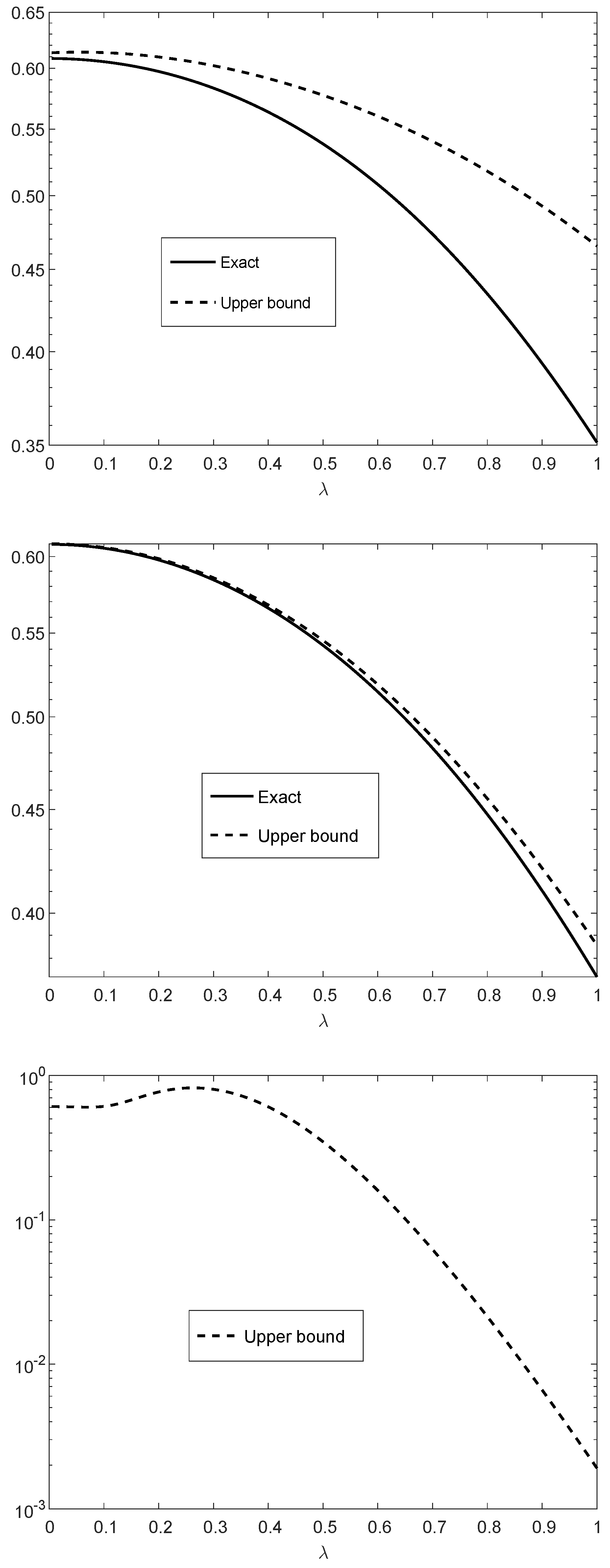
Figure 1 illustrates the upper and lower bounds in (116) and (117) with $\alpha =1$, $p_i\equiv \frac{1}{4}$, $q_i\equiv \frac{1}{2}$ and ${\delta }_i\equiv 0.110$ for all i, and $n\in \{1,10,50\}$. In the special case where $\left\{{\delta }_i\right\}$ are fixed for all i, the communication channel is a time-invariant BSC whose capacity is equal to $\frac{1}{2}$ bit per channel use.

By referring to the upper and middle plots of Figure 1, if $n=1$ or $n=10$, then the exact values of the differences of the $f_{\alpha }$-divergences in the right side of (116) are calculated numerically, being compared to the lower and upper bounds in the left side of (116) and the right side of (117) respectively. Since the $f_{\alpha }$-divergence does not tensorize, the computation of the exact value of each of the two $f_{\alpha }$-divergences in the right side of (116) involves a pre-computation of $2^n$ probabilities for each of the probability mass functions $P_{X^n}$, $Q_{X^n}$, $P_{Y^n}$ and $Q_{Y^n}$; this computation is prohibitively complex unless n is small enough.

We now apply the bound in Theorem 4. In view of (51), (54), (55) and (73), for all $\lambda \in (0,1]$ and $\alpha \ge {\mathrm{e}}^{-\frac{3}{2}}$,

$$\begin{array}{cc}\hfill & \frac{D_{f_{\alpha }}\left(R_{Y^n}^{\left(\lambda \right)}\parallel Q_{Y^n}\right)}{D_{f_{\alpha }}\left(R_{X^n}^{\left(\lambda \right)}\parallel Q_{X^n}\right)}\hfill \end{array}$$

$$\begin{array}{cc}\hfill & \le \frac{{\kappa }_{\alpha }\left({\xi }_1(n,\lambda ),{\xi }_2(n,\lambda )\right)}{f_{\alpha }\left(0\right)+f_{\alpha }^{\prime }\left(1\right)}\frac{{\displaystyle \prod _{i=1}^n}\left(1+{\lambda }^2{\chi }^2(P_{Y_i}\parallel Q_{Y_i}\right))-1}{{\displaystyle \prod _{i=1}^n}\left(1+{\lambda }^2{\chi }^2(P_{X_i}\parallel Q_{X_i}\right))-1}\hfill \end{array}$$

(125)

$$\begin{array}{cc}\hfill & =\frac{f_{\alpha }\left({\xi }_2(n,\lambda )\right)+f_{\alpha }^{\prime }\left(1\right)\left(1-{\xi }_2(n,\lambda )\right)}{{\left({\xi }_2(n,\lambda )-1\right)}^2\left(f_{\alpha }\left(0\right)+f_{\alpha }^{\prime }\left(1\right)\right)}·\frac{{\displaystyle \prod _{i=1}^n}\left(1+{\displaystyle \frac{{\lambda }^2{(p_i\ast {\delta }_i-q_i\ast {\delta }_i)}^2}{(q_i\ast {\delta }_i)(1-q_i\ast {\delta }_i)}}\right)-1}{{\displaystyle \prod _{i=1}^n}\left(1+{\displaystyle \frac{{\lambda }^2{(p_i-q_i)}^2}{q_i(1-q_i)}}\right)-1},\hfill \end{array}$$

(126)

where ${\xi }_1(n,\lambda )\in [0,1)$ and ${\xi }_2(n,\lambda )\in (1,\infty )$ are given in (122) and (123), respectively, and for $t\ge 0$,

$$\begin{array}{c}{f}_{\alpha }\left(t\right)+f_{\alpha }^{\prime }\left(1\right)(1-t)\hfill \\ ={(\alpha +t)}^{2}log(\alpha +t)-{(\alpha +1)}^{2}log(\alpha +1)+\left[2(\alpha +1)log(\alpha +1)+(\alpha +1)log\mathrm{e}\right](1-t).\hfill \end{array}$$

(127)

Figure 2 illustrates the upper bound on $\frac{D_{f_{\alpha }}(R_{Y^n}^{\left(\lambda \right)}\parallel Q_{Y^n})}{D_{f_{\alpha }}(R_{X^n}^{\left(\lambda \right)}\parallel Q_{X^n})}$ (see (125)–(127)) as a function of $\lambda \in (0,1]$. It refers to the case where $p_i\equiv \frac{1}{4}$, $q_i\equiv \frac{1}{2}$, and ${\delta }_i\equiv 0.110$ for all i (similarly to Figure 1). The upper and middle plots correspond to $n=10$ with $\alpha =10$ and $\alpha =100$, respectively; the middle and lower plots correspond to $\alpha =100$ with $n=10$ and $n=100$, respectively. The bounds in the upper and middle plots are compared to their exact values since their numerical computations are feasible for $n=10$. It is observed from the numerical comparisons for $n=10$ (see the upper and middle plots in Figure 2) that the upper bounds are informative, especially for large values of $\alpha$ where the $f_{\alpha }$-divergence becomes closer to a scaled version of the ${\chi }^2$-divergence (see Item (e) in Theorem 5).

3.2. Illustration of Theorems 3 and 5

Following the application of the data-processing inequalities in Theorems 2 and 4 to a class of f-divergences (see Section 3.1), some interesting properties of this class are introduced in Theorem 5.

For $\alpha \ge {\mathrm{e}}^{-\frac{3}{2}}$, let $d_{f_{\alpha }}:{(0,1)}^2\to [0,\infty )$ be the binary $f_{\alpha }$-divergence (see (55)), defined as

$$\begin{array}{cc}\hfill d_{f_{\alpha }}(p\parallel q)& :=D_{f_{\alpha }}\left(\mathrm{Bernoulli}\left(p\right)\parallel \mathrm{Bernoulli}\left(q\right)\right)\hfill \\ & =q{\left(\alpha +\frac{p}{q}\right)}^{2}log\left(\alpha +\frac{p}{q}\right)+(1-q){\left(\alpha +\frac{1-p}{1-q}\right)}^{2}log\left(\alpha +\frac{1-p}{1-q}\right)\hfill \end{array}$$

(128)

$$\begin{array}{cc}\hfill & -{(\alpha +1)}^{2}log(\alpha +1),\forall (p,q)\in {(0,1)}^2.\hfill \end{array}$$

(129)

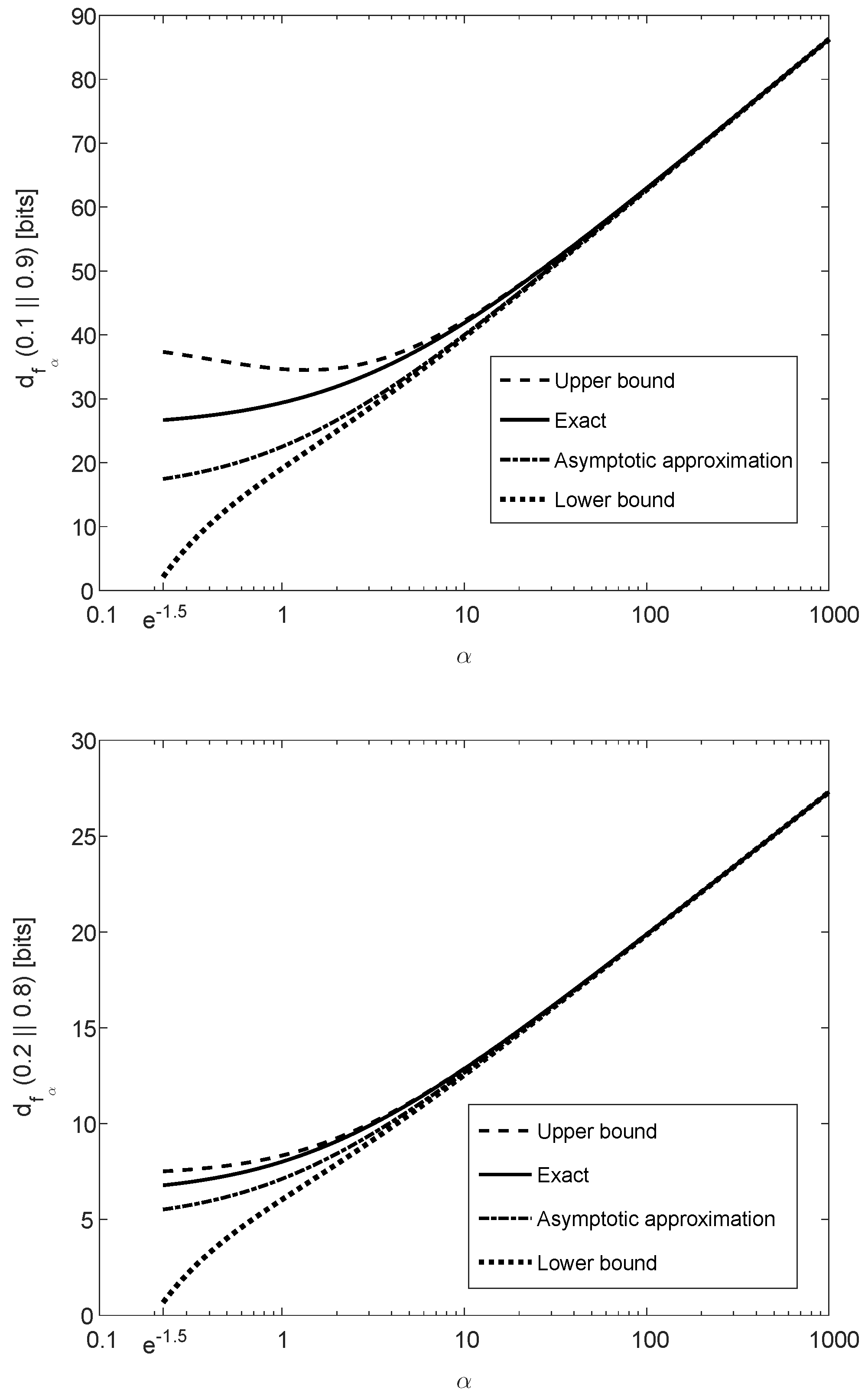
Theorem 5 is illustrated in Figure 3, showing that $d_{f_{\alpha }}(p\parallel q)$ is monotonically increasing as a function of $\alpha \ge {\mathrm{e}}^{-\frac{3}{2}}$ (note that the concavity in $\alpha$ is not reflected from these plots because the horizontal axis of $\alpha$ is in logarithmic scaling). The binary divergence $d_{f_{\alpha }}(p\parallel q)$ is also compared in Figure 3 with its lower and upper bounds in (61) and (65), respectively, illustrating that these bounds are both asymptotically tight for large values of $\alpha$. The asymptotic approximation of $d_{f_{\alpha }}(p\parallel q)$ for large $\alpha$, expressed as a function of $\alpha$ and ${\chi }^2(p\parallel q)$ (see (66)), is also depicted in Figure 3. The upper and lower plots in Figure 3 refer, respectively, to $(p,q)=(0.1,0.9)$ and $(0.2,0.8)$; a comparison of these plots show a better match between the exact value of the binary divergence, its upper and lower bounds, and its asymptotic approximation when the values of p and q are getting closer.

In view of the results in (66) and (68), it is interesting to note that the asymptotic value of $D_{f_{\alpha }}(P\parallel Q)$ for large values of $\alpha$ is also the exact scaling of this f-divergence for any finite value of $\alpha \ge {\mathrm{e}}^{-\frac{3}{2}}$ when the probability mass functions P and Q are close enough to each other.

We next consider the ratio of the contraction coefficients $\frac{{\mu }_{f_{\alpha }}(Q_X,W_{Y|X})}{{\mu }_{{\chi }^2}(Q_X,W_{Y|X})}$ where $Q_X$ is finitely supported on $\mathcal{X}$ and it is not a point mass (i.e., $\left|\mathcal{X}\right|\ge 2$), and $W_{Y|X}$ is arbitrary. For all $\alpha \ge {\mathrm{e}}^{-\frac{3}{2}}$,

$$\begin{array}{c}\hfill 1\le \frac{{\mu }_{f_{\alpha }}(Q_X,W_{Y|X})}{{\mu }_{{\chi }^2}(Q_X,W_{Y|X})}\le \frac{f_{\alpha }\left(\xi \right)+f_{\alpha }^{\prime }\left(1\right)(1-\xi )}{{(\xi -1)}^2\left(f_{\alpha }\left(0\right)+f_{\alpha }^{\prime }\left(1\right)\right)},\end{array}$$

(130)

where $f_{\alpha }:(0,\infty )\to \mathbb{R}$ is given in (55), and

$$\begin{array}{c}\hfill \xi :=\frac{1}{{\displaystyle \underset{x\in \mathcal{X}}{min}}{Q}_X\left(x\right)}\in \left[\right|\mathcal{X}|,\infty ).\end{array}$$

(131)

The left-side inequality in (130) is due to ([25], Theorem 2) (see Proposition 2), and the right-side inequality in (130) holds due to (53) and (73).

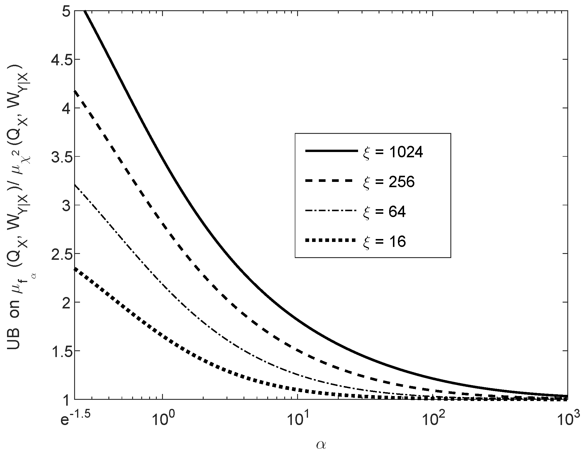
Figure 4 shows the upper bound on the ratio of contraction coefficients $\frac{{\mu }_{f_{\alpha }}(Q_X,W_{Y|X})}{{\mu }_{{\chi }^2}(Q_X,W_{Y|X})}$, as it is given in the right-side inequality of (130), as a function of the parameter $\alpha \ge {\mathrm{e}}^{-\frac{3}{2}}$. The curves in Figure 4 correspond to different values of $\xi \in [|\mathcal{X}|,\infty )$, as it is given in (131); these upper bounds are monotonically decreasing in $\alpha$, and they asymptotically tend to 1 as we let $\alpha \to \infty$. Hence, in view of the left-side inequality in (130), the upper bound on the ratio of the contraction coefficients (in the right-side inequality) is asymptotically tight in $\alpha$. The fact that the ratio of the contraction coefficients in the middle of (130) tends asymptotically to 1, as $\alpha$ gets large, is not directly implied by Item (e) of Theorem 5. The latter implies that, for fixed probability mass functions P and Q and for sufficiently large $\alpha$,

$$\begin{array}{c}\hfill D_{f_{\alpha }}(P\parallel Q)\approx \left[log(\alpha +1)+\frac{3}{2}log\mathrm{e}\right]{\chi }^2(P\parallel Q);\end{array}$$

(132)

however, there is no guarantee that for fixed Q and sufficiently large $\alpha$, the approximation in (132) holds for all P. By the upper bound in the right side of (130), it follows however that ${\mu }_{f_{\alpha }}(Q_X,W_{Y|X})$ tends asymptotically (as we let $\alpha \to \infty$) to the contraction coefficient of the ${\chi }^2$ divergence.

3.3. Illustration of Theorem 7 and Further Results

Theorem 7 provides upper and lower bounds on an f-divergence, $D_f(Q\parallel U_n)$, from any probability mass function Q supported on a finite set of cardinality n to an equiprobable distribution over this set. We apply in the following, the exact formula for

$$\begin{array}{c}\hfill d_f\left(\rho \right):={\displaystyle \underset{n\to \infty }{lim}}{\displaystyle \underset{Q\in {\mathcal{P}}_n\left(\rho \right)}{max}}{D}_f(Q\parallel U_n),\rho \ge 1\end{array}$$

(133)

to several important f-divergences. From (87),

$$\begin{array}{c}\hfill d_f\left(\rho \right)={\displaystyle \underset{x\in [0,1]}{max}}\left\{xf\left(\frac{\rho }{1+(\rho -1)x}\right)+(1-x)f\left(\frac{1}{1+(\rho -1)x}\right)\right\},\rho \ge 1.\end{array}$$

(134)

Since f is a convex function on $(0,\infty )$ with $f\left(1\right)=0$, Jensen’s inequality implies that the function which is subject to maximization in the right-side of (134) is non-negative over the interval $[0,1]$. It is equal to zero at the endpoints of the interval $[0,1]$, so the maximum over this interval is attained at an interior point. Note also that, in view of Items (d) and (e) of Theorem 7, the exact asymptotic expression in (134) satisfies

$$\begin{array}{c}\hfill {\displaystyle \underset{Q\in {\mathcal{P}}_n\left(\rho \right)}{max}}{D}_f(Q\parallel U_n)\le d_f\left(\rho \right),\forall n\in \{2,3,\dots \},\rho \ge 1.\end{array}$$

(135)

3.3.1. Total Variation Distance

This distance is an f-divergence with $f\left(t\right):=|t-1|$ for $t>0$. Substituting f into (134) gives

$$\begin{array}{c}\hfill d_f\left(\rho \right)={\displaystyle \underset{x\in [0,1]}{max}}\left\{\frac{2(\rho -1)x(1-x)}{1+(\rho -1)x}\right\}.\end{array}$$

(136)

By setting to zero the derivative of the function which is subject to maximization in the right side of (136), it can be verified that the maximizer over this interval is equal to $x=\frac{1}{1+\sqrt{\rho }}$, which implies that

$$\begin{array}{c}\hfill d_f\left(\rho \right)=\frac{2(\sqrt{\rho }-1)}{\sqrt{\rho }+1},\forall \rho \ge 1.\end{array}$$

(137)

3.3.2. Alpha Divergences

The class of Alpha divergences forms a parametric subclass of the f-divergences, which includes in particular the relative entropy, ${\chi }^2$-divergence, and the squared-Hellinger distance. For $\alpha \in \mathbb{R}$, let

$$\begin{array}{c}\hfill D_{\mathrm{A}}^{\left(\alpha \right)}(P\parallel Q):=D_{u_{\alpha }}(P\parallel Q),\end{array}$$

(138)

where $u_{\alpha }:(0,\infty )\to \mathbb{R}$ is a non-negative and convex function with $u_{\alpha }\left(1\right)=0$, which is defined for $t>0$ as follows (see ([8], Chapter 2), followed by studies in, e.g., [10,16,43,44,45]):

$$u_{\alpha }\left(t\right):=\{\begin{array}{cc}\frac{t^{\alpha }-\alpha (t-1)-1}{\alpha (\alpha -1)},\hfill & \alpha \in (-\infty ,0)\cup (0,1)\cup (1,\infty ),\hfill \\ t{log}_{\mathrm{e}}t+1-t,\hfill & \alpha =1,\hfill \\ -{log}_{\mathrm{e}}t,\hfill & \alpha =0.\hfill \end{array}$$

(139)

The functions $u_0$ and $u_1$ are defined in the right side of (139) by a continuous extension of $u_{\alpha }$ at $\alpha =0$ and $\alpha =1$, respectively. The following relations hold (see, e.g., ([44], (10)–(13))):

$$\begin{array}{c}{D}_{\mathrm{A}}^{\left(1\right)}(P\parallel Q)=\frac{1}{log\mathrm{e}}D(P\parallel Q),\hfill \end{array}$$

(140)

$$\begin{array}{c}{D}_{\mathrm{A}}^{\left(0\right)}(P\parallel Q)=\frac{1}{log\mathrm{e}}D(Q\parallel P),\hfill \end{array}$$

(141)

$$\begin{array}{c}{D}_{\mathrm{A}}^{\left(2\right)}(P\parallel Q)=\frac{1}{2}{\chi }^2(P\parallel Q),\hfill \end{array}$$

(142)

$$\begin{array}{c}{D}_{\mathrm{A}}^{(-1)}(P\parallel Q)=\frac{1}{2}{\chi }^2(Q\parallel P),\hfill \end{array}$$

(143)

$$\begin{array}{c}{D}_{\mathrm{A}}^{\left(\frac{1}{2}\right)}(P\parallel Q)=4{\mathcal{H}}^2(P\parallel Q).\hfill \end{array}$$

(144)

Substituting $f:=u_{\alpha }$ (see (139)) into the right side of (134) gives that

$$\begin{array}{cc}\hfill \Delta (\alpha ,\rho )& :=d_{u_{\alpha }}\left(\rho \right)\hfill \end{array}$$

(145)

$$\begin{array}{cc}\hfill & ={\displaystyle \underset{n\to \infty }{lim}}{\displaystyle \underset{Q\in {\mathcal{P}}_n\left(\rho \right)}{max}}{D}_{\mathrm{A}}^{\left(\alpha \right)}(Q\parallel U_n)\hfill \end{array}$$

(146)

$$\begin{array}{cc}\hfill & ={\displaystyle \underset{x\in [0,1]}{max}}\left\{\frac{1+({\rho }^{\alpha }-1)x}{{\left(1+(\rho -1)x\right)}^{\alpha }}-1\right\}.\hfill \end{array}$$

(147)

Setting to zero the derivative of the function which is subject to maximization in the right side of (147) gives

$$\begin{array}{c}\hfill x=x^{\ast }:=\frac{1+\alpha (\rho -1)-{\rho }^{\alpha }}{(1-\alpha )(\rho -1)({\rho }^{\alpha }-1)},\end{array}$$

(148)

where it can be verified that $x^{\ast }\in (0,1)$ for all $\alpha \in (-\infty ,0)\cup (0,1)\cup (1,\infty )$ and $\rho >1$. Substituting (148) into the right side of (147) gives that, for all such $\alpha$ and $\rho$,

$$\begin{array}{c}\hfill \Delta (\alpha ,\rho )=\frac{1}{\alpha (\alpha -1)}\left[\frac{{(1-\alpha )}^{\alpha -1}{({\rho }^{\alpha }-1)}^{\alpha }{(\rho -{\rho }^{\alpha })}^{1-\alpha }}{(\rho -1){\alpha }^{\alpha }}-1\right].\end{array}$$

(149)

By a continuous extension of $\Delta (\alpha ,\rho )$ in (149) at $\alpha =1$ and $\alpha =0$, it follows that for all $\rho >1$

$$\begin{array}{c}\hfill \Delta (1,\rho )=\Delta (0,\rho )=\frac{\rho log\rho }{\rho -1}-log\left(\frac{\mathrm{e}\rho {log}_{\mathrm{e}}\rho }{\rho -1}\right).\end{array}$$

(150)

Consequently, for all $\rho >1$,

$$\begin{array}{cc}\hfill {\displaystyle \underset{n\to \infty }{lim}}{\displaystyle \underset{Q\in {\mathcal{P}}_n\left(\rho \right)}{max}}D(Q\parallel U_n)& =log\mathrm{e}{\displaystyle \underset{n\to \infty }{lim}}{\displaystyle \underset{Q\in {\mathcal{P}}_n\left(\rho \right)}{max}}{D}_{\mathrm{A}}^{\left(1\right)}(Q\parallel U_n)\hfill \end{array}$$

(151)

$$\begin{array}{cc}\hfill & =\Delta (1,\rho )log\mathrm{e}\hfill \end{array}$$

(152)

$$\begin{array}{cc}\hfill & =\frac{\rho log\rho }{\rho -1}-log\left(\frac{\mathrm{e}\rho {log}_{\mathrm{e}}\rho }{\rho -1}\right),\hfill \end{array}$$

(153)

where (151) holds due to (140); (152) is due to (146), and (153) holds due to (150). This sharpens the result in ([33], Theorem 2) for the relative entropy from the equiprobable distribution, $D(Q\parallel U_n)=logn-H\left(Q\right)$, by showing that the bound in ([33], (7)) is asymptotically tight as we let $n\to \infty$. The result in ([33], Theorem 2) can be further tightened for finite n by applying the result in Theorem 7 (d) with $f\left(t\right):=u_1\left(t\right)log\mathrm{e}=tlogt+(1-t)log\mathrm{e}$ for all $t>0$ (although, unlike the asymptotic result in (149), the refined bound for a finite n does not lend itself to a closed-form expression as a function of n; see also ([34], Remark 3), which provides such a refinement of the bound on $D(Q\parallel U_n)$ for finite n in a different approach).

From (141), (146) and (150), it follows similarly to (153) that for all $\rho >1$

$$\begin{array}{cc}\hfill {\displaystyle \underset{n\to \infty }{lim}}{\displaystyle \underset{Q\in {\mathcal{P}}_n\left(\rho \right)}{max}}D(U_n\parallel Q)& =\Delta (0,\rho )log\mathrm{e}\hfill \end{array}$$

(154)

$$\begin{array}{cc}\hfill & =\frac{\rho log\rho }{\rho -1}-log\left(\frac{\mathrm{e}\rho {log}_{\mathrm{e}}\rho }{\rho -1}\right).\hfill \end{array}$$

(155)

It should be noted that in view of the one-to-one correspondence between the Rényi divergence and the Alpha divergence of the same order $\alpha$ where, for $\alpha \ne 1$,

$$\begin{array}{c}\hfill D_{\alpha }(P\parallel Q)=\frac{1}{\alpha -1}log\left(1+\alpha (\alpha -1)D_{\mathrm{A}}^{\left(\alpha \right)}(P\parallel Q)\right),\end{array}$$

(156)

the asymptotic result in (149) can be obtained from ([34], Lemma 4) and vice versa; however, in [34], the focus is on the Rényi divergence from the equiprobable distribution, whereas the result in (149) is obtained by specializing the asymptotic expression in (134) for a general f-divergence. Note also that the result in ([34], Lemma 4) is restricted to $\alpha >0$, whereas the result in (149) and (150) covers all values of $\alpha \in \mathbb{R}$.

In view of (146), (149), (153), (155), and the special cases of the Alpha divergences in (140)–(144), it follows that for all $\rho >1$ and for every integer $n\ge 2$

$$\begin{array}{cc}\hfill {\displaystyle \underset{Q\in {\mathcal{P}}_n\left(\rho \right)}{max}}D(Q\parallel U_n)& \le \Delta (1,\rho )log\mathrm{e}=\frac{\rho log\rho }{\rho -1}-log\left(\frac{\mathrm{e}\rho {log}_{\mathrm{e}}\rho }{\rho -1}\right),\hfill \end{array}$$

(157)

$$\begin{array}{cc}\hfill {\displaystyle \underset{Q\in {\mathcal{P}}_n\left(\rho \right)}{max}}D(U_n\parallel Q)& \le \Delta (0,\rho )log\mathrm{e}=\frac{\rho log\rho }{\rho -1}-log\left(\frac{\mathrm{e}\rho {log}_{\mathrm{e}}\rho }{\rho -1}\right),\hfill \end{array}$$

(158)

$$\begin{array}{cc}\hfill {\displaystyle \underset{Q\in {\mathcal{P}}_n\left(\rho \right)}{max}}{\chi }^2(Q\parallel U_n)& \le 2\Delta (2,\rho )=\frac{{(\rho -1)}^2}{4\rho },\hfill \end{array}$$

(159)

$$\begin{array}{cc}\hfill {\displaystyle \underset{Q\in {\mathcal{P}}_n\left(\rho \right)}{max}}{\chi }^2(U_n\parallel Q)& \le 2\Delta (-1,\rho )=\frac{{(\rho -1)}^2}{4\rho },\hfill \end{array}$$

(160)

$$\begin{array}{cc}\hfill {\displaystyle \underset{Q\in {\mathcal{P}}_n\left(\rho \right)}{max}}{\mathcal{H}}^2(Q\parallel U_n)& \le \frac{1}{4}\Delta (\frac{1}{2},\rho )=\frac{{(\sqrt[4]{\rho }-1)}^2}{\sqrt{\rho }+1},\hfill \end{array}$$

(161)

and the upper bounds on the right sides of (157)–(161) are asymptotically tight in the limit where n tends to infinity.

The next result characterizes the function $\Delta :(0,\infty )\times (1,\infty )\to \mathbb{R}$ as it is given in (149) and (150).

Theorem 9.

The function Δ satisfies the following properties:

(a) 

For every $\rho >1$, $\Delta (\alpha ,\rho )$ is a convex function of α over the real line, and it is symmetric around $\alpha =\frac{1}{2}$ with a global minimum at $\alpha =\frac{1}{2}$.

(b) 

The following inequalities hold:

$$\begin{array}{cc}\hfill & \alpha \Delta (\alpha ,\rho )\le \beta \Delta (\beta ,\rho ),0<\alpha \le \beta <\infty ,\hfill \end{array}$$

(162)

$$\begin{array}{cc}\hfill & (1-\beta )\Delta (\beta ,\rho )\le (1-\alpha )\Delta (\alpha ,\rho ),-\infty <\alpha \le \beta <1.\hfill \end{array}$$

(163)

(c) 

For every $\alpha \in \mathbb{R}$, $\Delta (\alpha ,\rho )$ is monotonically increasing and continuous in $\rho \in (1,\infty )$, and ${\displaystyle \underset{\rho \to 1^{+}}{lim}}\Delta (\alpha ,\rho )=0$.

Proof. 

See Appendix H.1.  □

Remark 6.

The symmetry of $\Delta (\alpha ,\rho )$ around $\alpha =\frac{1}{2}$ (see Theorem 9 (a)) is not implied by the following symmetry property of the Alpha divergence around $\alpha =\frac{1}{2}$ (see, e.g., ([8], p. 36)):

$$\begin{array}{c}\hfill D_{\mathrm{A}}^{(\frac{1}{2}+\alpha )}(P\parallel Q)=D_{\mathrm{A}}^{(\frac{1}{2}-\alpha )}(Q\parallel P).\end{array}$$

(164)

Relying on Theorem 9, the following corollary gives a similar result to (146) where the order of Q and $U_n$ in $D_{\mathrm{A}}^{\left(\alpha \right)}(·\parallel ·)$ is switched.

Corollary 1.

For all $\alpha \in \mathbb{R}$ and $\rho >1$,

$$\begin{array}{c}\hfill {\displaystyle \underset{n\to \infty }{lim}}{\displaystyle \underset{Q\in {\mathcal{P}}_n\left(\rho \right)}{max}}{D}_{\mathrm{A}}^{\left(\alpha \right)}(U_n\parallel Q)=\Delta (\alpha ,\rho ).\end{array}$$

(165)

Proof. 

See Appendix H.2.  □

We next further exemplify Theorem 7 for the relative entropy. Let $f\left(t\right):=tlogt+(1-t)log\mathrm{e}$ for $t>0$. Then, $f^{″}\left(t\right)=\frac{log\mathrm{e}}{t}$, so the bounds on the second derivative of f over the interval $[\frac{1}{\rho },\rho ]$ are given by $M=\rho log\mathrm{e}$ and $m=\frac{log\mathrm{e}}{\rho }$. Theorem 7 (h) gives the following bounds:

$$\begin{array}{c}\hfill \frac{\left({n\parallel Q\parallel }_2^2-1\right)log\mathrm{e}}{2\rho }\le D(Q\parallel U_n)\le \frac{\rho \left({n\parallel Q\parallel }_2^2-1\right)log\mathrm{e}}{2}.\end{array}$$

(166)

From ([33], Theorem 2) (and (157)),

$$\begin{array}{c}\hfill D(Q\parallel U_n)\le \frac{\rho log\rho }{\rho -1}-log\left(\frac{\mathrm{e}\rho {log}_{\mathrm{e}}\rho }{\rho -1}\right).\end{array}$$

(167)

Furthermore, (96) gives that

$$\begin{array}{c}\hfill D(Q\parallel U_n)\le \frac{1}{8}{(\rho -1)}^{2}log\mathrm{e},\end{array}$$

(168)

which, for $\rho >1$, is a looser bound in comparison to (167). It can be verified, however, that the dominant term in the Taylor series expansion (around $\rho =1$) of the right side of (167) coincides with the right side of (168), so the bounds scale similarly for small values of $\rho \ge 1$.

Suppose that we wish to assert that, for every integer $n\ge 2$ and for all probability mass functions $Q\in {\mathcal{P}}_n\left(\rho \right)$, the condition

$$\begin{array}{c}\hfill D(Q\parallel U_n)\le dlog\mathrm{e}\end{array}$$

(169)

holds with a fixed $d>0$. Due to the left side inequality in (89), this condition is equivalent to the requirement that

$$\begin{array}{c}\hfill {\displaystyle \underset{n\to \infty }{lim}}{\displaystyle \underset{Q\in {\mathcal{P}}_n\left(\rho \right)}{max}}D(Q\parallel U_n)\le dlog\mathrm{e}.\end{array}$$

(170)

Due to the asymptotic tightness of the upper bound in the right side of (157) (as we let $n\to \infty$), requiring that this upper bound is not larger than $dlog\mathrm{e}$ is necessary and sufficient for the satisfiability of (169) for all n and $Q\in {\mathcal{P}}_n\left(\rho \right)$. This leads to the analytical solution $\rho \le {\rho }_{max}^{\left(1\right)}\left(d\right)$ with (see Appendix I)

$$\begin{array}{c}\hfill {\rho }_{max}^{\left(1\right)}\left(d\right):=\frac{W_{-1}\left(-{\mathrm{e}}^{-d-1}\right)}{W_0\left(-{\mathrm{e}}^{-d-1}\right)},\end{array}$$

(171)

where $W_0$ and $W_{-1}$ denote, respectively, the principal and secondary real branches of the Lambert W function [37]. Requiring the stronger condition where the right side of (168) is not larger than $dlog\mathrm{e}$ leads to the sufficient solution $\rho \le {\rho }_{max}^{\left(2\right)}$ with the simple expression

$$\begin{array}{c}\hfill {\rho }_{max}^{\left(2\right)}\left(d\right):=1+\sqrt{8d}.\end{array}$$

(172)

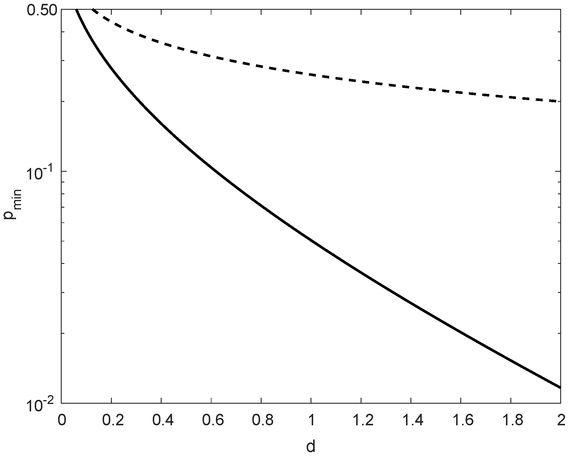
In comparison to ${\rho }_{max}^{\left(1\right)}$ in (171), ${\rho }_{max}^{\left(2\right)}$ in (172) is more insightful; these values nearly coincide for small values of $d>0$, providing in that case the same range of possible values of $\rho$ for asserting the satisfiability of condition (169). As it is shown in Figure 5, for $d\le 0.01$, the difference between the maximal values of $\rho$ in (171) and (172) is marginal, though in general ${\rho }_{max}^{\left(1\right)}\left(d\right)>{\rho }_{max}^{\left(2\right)}\left(d\right)$ for all $d>0$.

3.3.3. The Subclass of f-Divergences in Theorem 5

This example refers to the subclass of f-divergences in Theorem 5. For these $f_{\alpha }$-divergences, with $\alpha \ge {\mathrm{e}}^{-\frac{3}{2}}$, substituting $f:=f_{\alpha }$ from (55) into the right side of (134) gives that for all $\rho \ge 1$

$$\begin{array}{cc}\hfill \Phi (\alpha ,\rho )& :=d_{f_{\alpha }}\left(\rho \right)\hfill \end{array}$$

(172)

$$\begin{array}{cc}\hfill & ={\displaystyle \underset{n\to \infty }{lim}}{\displaystyle \underset{Q\in {\mathcal{P}}_n\left(\rho \right)}{max}}{D}_{f_{\alpha }}(Q\parallel U_n)\hfill \\ \hfill & ={\displaystyle \underset{x\in [0,1]}{max}}\left\{x{\left(\alpha +\frac{\rho }{1+(\rho -1)x}\right)}^{2}log\left(\alpha +\frac{\rho }{1+(\rho -1)x}\right)-{(\alpha +1)}^{2}log(\alpha +1)\right.\hfill \end{array}$$

(173)

$$\begin{array}{cc}\hfill & \left.+(1-x){\left(\alpha +\frac{1}{1+(\rho -1)x}\right)}^{2}log\left(\alpha +\frac{1}{1+(\rho -1)x}\right)\right\}.\hfill \end{array}$$

(175)

The exact asymptotic expression in the right side of (175) is subject to numerical maximization.

We next provide two alternative closed-form upper bounds, based on Theorems 5 and 7, and study their tightness. The two upper bounds, for all $\alpha \ge {\mathrm{e}}^{-\frac{3}{2}}$ and $\rho \ge 1$, are given by (see Appendix J)

$$\begin{array}{cc}\hfill \Phi (\alpha ,\rho )& \le \left[log(\alpha +1)+\frac{3}{2}log\mathrm{e}-\frac{log\mathrm{e}}{\alpha +1}\right]\frac{{(\rho -1)}^2}{4\rho }\hfill \\ & +\frac{log\mathrm{e}}{81(\alpha +1)}{\left(\frac{(\rho -1)(2\rho +1)(\rho +2)}{\rho (\rho +1)}\right)}^2,\hfill \end{array}$$

(176)

and

$$\begin{array}{c}\hfill \Phi (\alpha ,\rho )\le \left[log(\alpha +\rho )+\frac{3}{2}log\mathrm{e}\right]\frac{{(\rho -1)}^2}{4\rho }.\end{array}$$

(177)

Suppose that we wish to assert that, for every integer $n\ge 2$ and for all probability mass functions $Q\in {\mathcal{P}}_n\left(\rho \right)$, the condition

$$\begin{array}{c}\hfill D_{f_{\alpha }}(Q\parallel U_n)\le dlog\mathrm{e}\end{array}$$

(178)

holds with a fixed $d>0$ and $\alpha \ge {\mathrm{e}}^{-\frac{3}{2}}$. Due to (173)–(174) and the left side inequality in (89), the satisfiability of the latter condition is equivalent to the requirement that

$$\begin{array}{c}\hfill \Phi (\alpha ,\rho )\le dlog\mathrm{e}.\end{array}$$

(179)

In order to obtain a sufficient condition for $\rho$ to satisfy (179), expressed as an explicit function of $\alpha$ and d, the upper bound in the right side of (176) is slightly loosened to

$$\begin{array}{c}\hfill \Phi (\alpha ,\rho )\le a{(\rho -1)}^2+bmin\{\rho -1,{(\rho -1)}^2\},\end{array}$$

(180)

where

$$\begin{array}{cc}\hfill & a:=\frac{4log\mathrm{e}}{81(\alpha +1)},\hfill \end{array}$$

(181)

$$\begin{array}{cc}\hfill & b:=\frac{1}{4}log(\alpha +1)+\frac{3}{8}log\mathrm{e},\hfill \end{array}$$

(182)

for all $\rho \ge 1$ and $\alpha \ge {\mathrm{e}}^{-\frac{3}{2}}$. The upper bounds in the right sides of (176), (177) and (180) are derived in Appendix J.

In comparison to (179), the stronger requirement that the right side of (180) is less than or equal to $dlog\mathrm{e}$ gives the sufficient condition

$$\begin{array}{c}\hfill \rho \le {\rho }_{max}(\alpha ,d):=max\left\{{\rho }_1(\alpha ,d),{\rho }_2(\alpha ,d)\right\},\end{array}$$

(183)

with

$$\begin{array}{cc}\hfill & {\rho }_1(\alpha ,d):=1+\frac{\sqrt{b^2+4adlog\mathrm{e}}-b}{2a},\hfill \end{array}$$

(184)

$$\begin{array}{cc}\hfill & {\rho }_2(\alpha ,d):=1+\sqrt{\frac{dlog\mathrm{e}}{a+b}}.\hfill \end{array}$$

(185)

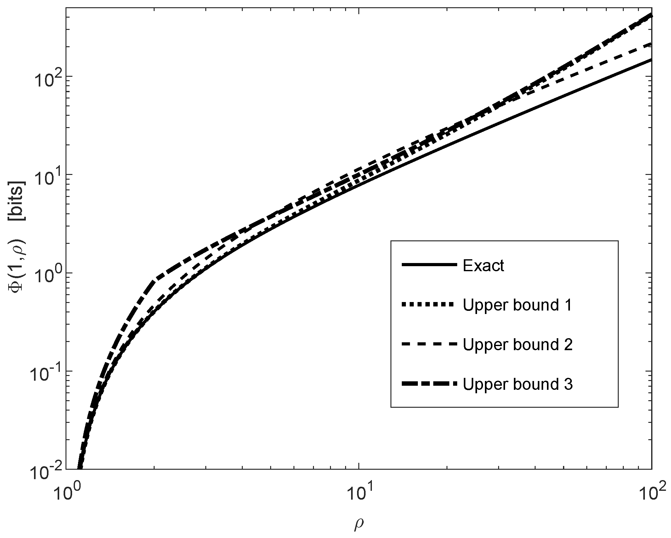
Figure 6 compares the exact expression in (175) with its upper bounds in (176), (177) and (180). These bounds show good match with the exact value, and none of the bounds in (176) and (177) is superseded by the other; the bound in (180) is looser than (176), and it is derived for obtaining the closed-form solution in (183)–(185). The bound in (176) is tighter than the bound in (177) for small values of $\rho \ge 1$, whereas the latter bound outperforms the first one for sufficiently large values of $\rho$. It has been observed numerically that the tightness of the bounds is improved by increasing the value of $\alpha$, and the range of parameters of $\rho$ over which the bound in (176) outperforms the second bound in (177) is enlarged when $\alpha$ is increased. It is also shown in Figure 6 that the bound in (176) and its loosened version in (180) almost coincide for sufficiently small values of $\rho$ (i.e., for $\rho$ is close to 1), and also for sufficiently large values of $\rho$.

3.4. An Interpretation of $u_f(·,·)$ in Theorem 7

We provide here an interpretation of $u_f(n,\rho )$ in (77), for $\rho >1$ and an integer $n\ge 2$; note that $u_f(n,1)\equiv 0$ since ${\mathcal{P}}_n\left(1\right)=\left\{U_n\right\}$. Before doing so, recall that (82) introduces an identity which significantly simplifies the numerical calculation of $u_f(n,\rho )$, and (85) gives (asymptotically tight) upper and lower bounds.

The following result relies on the variational representation of f-divergences.

Theorem 10.

Let $f:(0,\infty )\to \mathbb{R}$ be convex with $f\left(1\right)=0$, and let $\overline{f}:\mathbb{R}\to \mathbb{R}\cup \{\infty \}$ be the convex conjugate function of f (a.k.a. the Fenchel-Legendre transform of f), i.e.,

$$\begin{array}{c}\hfill \overline{f}\left(x\right):={\displaystyle \underset{t>0}{sup}}\left\{tx-f\left(t\right)\right\},x\in \mathbb{R}.\end{array}$$

(186)

Let $\rho >1$, and define ${\mathcal{A}}_n:=\{1,\dots ,n\}$ for an integer $n\ge 2$. Then, the following holds:

(a) 

For every $P\in {\mathcal{P}}_n\left(\rho \right)$, a random variable $X\sim P$, and a function $g:{\mathcal{A}}_n\to \mathbb{R}$,

$$\begin{array}{c}\hfill \mathbb{E}\left[g\left(X\right)\right]\le u_f(n,\rho )+\frac{1}{n}{\displaystyle \sum _{i=1}^n}\overline{f}\left(g\left(i\right)\right).\end{array}$$

(187)

(b) 

There exists $P\in {\mathcal{P}}_n\left(\rho \right)$ such that, for every $\epsilon >0$, there is a function $g_{\epsilon }:{\mathcal{A}}_n\to \mathbb{R}$ which satisfies

$$\begin{array}{c}\hfill \mathbb{E}\left[g_{\epsilon }\left(X\right)\right]\ge u_f(n,\rho )+\frac{1}{n}{\displaystyle \sum _{i=1}^n}\overline{f}\left(g_{\epsilon }\left(i\right)\right)-\epsilon ,\end{array}$$

(188)

with $X\sim P$.

Proof. 

See Appendix K.  □

Remark 7.

The proof suggests a constructive way to obtain, for an arbitrary $\epsilon >0$, a function $g_{\epsilon }$ which satisfies (188).

4. Applications in Information Theory and Statistics

4.1. Bounds on the List Decoding Error Probability with f-Divergences

The minimum probability of error of a random variable X given Y, denoted by ${\epsilon }_{X|Y}$, can be achieved by a deterministic function (maximum-a-posteriori decision rule) ${\mathcal{L}}^{\ast }:\mathcal{Y}\to \mathcal{X}$ (see [42]):

$$\begin{array}{cc}\hfill {\epsilon }_{X|Y}& ={\displaystyle \underset{\mathcal{L}:\mathcal{Y}\to \mathcal{X}}{min}}\mathbb{P}[X\ne \mathcal{L}\left(Y\right)]\hfill \end{array}$$

(189)

$$\begin{array}{cc}\hfill & =\mathbb{P}[X\ne {\mathcal{L}}^{\ast }\left(Y\right)]\hfill \end{array}$$

(190)

$$\begin{array}{cc}\hfill & =1-\mathbb{E}\left[{\displaystyle \underset{x\in \mathcal{X}}{max}}{P}_{X|Y}\left(x\right|Y)\right].\hfill \end{array}$$

(191)

Fano’s inequality [46] gives an upper bound on the conditional entropy $H\left(X\right|Y)$ as a function of ${\epsilon }_{X|Y}$ (or, otherwise, providing a lower bound on ${\epsilon }_{X|Y}$ as a function of $H\left(X\right|Y\left)\right)$ when X takes a finite number of possible values.

The list decoding setting, in which the hypothesis tester is allowed to output a subset of given cardinality, and an error occurs if the true hypothesis is not in the list, has great interest in information theory. A generalization of Fano’s inequality to list decoding, in conjunction with the blowing-up lemma ([17], Lemma 1.5.4), leads to strong converse results in multi-user information theory. This approach was initiated in ([47], Section 5) (see also ([48], Section 3.6)). The main idea of the successful combination of these two tools is that, given a code, it is possible to blow-up the decoding sets in a way that the probability of decoding error can be as small as desired for sufficiently large blocklengths; since the blown-up decoding sets are no longer disjoint, the resulting setup is a list decoder with sub-exponential list size (as a function of the block length).

In statistics, Fano’s-type lower bounds on Bayes and minimax risks, expressed in terms of f-divergences, are derived in [49,50].

In this section, we further study the setup of list decoding, and derive bounds on the average list decoding error probability. We first consider the special case where the list size is fixed (see Section 4.1.1), and then move to the more general case of a list size which depends on the channel observation (see Section 4.1.2).

4.1.1. Fixed-Size List Decoding

A generalization of Fano’s inequality for fixed-size list decoding is given in ([42], (139)), expressed as a function of the conditional Shannon entropy (strengthening ([51], Lemma 1)). A further generalization in this setup, which is expressed as a function of the Arimoto-Rényi conditional entropy with an arbitrary positive order (see Definition 9), is provided in ([42], Theorem 8).

The next result provides a generalized Fano’s inequality for fixed-size list decoding, expressed in terms of an arbitrary f-divergence. Some earlier results in the literature are reproduced from the next result, followed by its strengthening as an application of Theorem 1.

Theorem 11.

Let $P_{XY}$ be a probability measure defined on $\mathcal{X}\times \mathcal{Y}$ with $\left|\mathcal{X}\right|=M$. Consider a decision rule $\mathcal{L}:\mathcal{Y}\to \left(\genfrac{}{}{0pt}{}{\mathcal{X}}{L}\right)$, where $\left(\genfrac{}{}{0pt}{}{\mathcal{X}}{L}\right)$ stands for the set of subsets of $\mathcal{X}$ with cardinality L, and $L<M$ is fixed. Denote the list decoding error probability by $P_{\mathcal{L}}:=\mathbb{P}\left[X\notin \mathcal{L}\left(Y\right)\right]$. Let $U_M$ denote an equiprobable probability mass function on $\mathcal{X}$. Then, for every convex function $f:(0,\infty )\to \mathbb{R}$ with $f\left(1\right)=0$,

$$\begin{array}{c}\hfill \mathbb{E}\left[D_f\left(P_{X|Y}(·|Y)\parallel U_M\right)\right]\ge \frac{L}{M}f\left(\frac{M(1-P_{\mathcal{L}})}{L}\right)+\left(1-\frac{L}{M}\right)f\left(\frac{M{P}_{\mathcal{L}}}{M-L}\right).\end{array}$$

(192)

Proof. 

See Appendix L.  □

Remark 8.

The case where $L=1$ (i.e., a decoder with a single output) gives ([50], (5)).

As consequences of Theorem 11, we first reproduce some earlier results as special cases.

Corollary 2

([42] (139)). Under the assumptions in Theorem 11,

$$\begin{array}{c}\hfill H\left(X\right|Y)\le logM-d\left(P_{\mathcal{L}}\parallel 1-\frac{L}{M}\right)\end{array}$$

(193)

where $d(·\parallel ·):[0,1]\times [0,1]\to [0,+\infty ]$ denotes the binary relative entropy, defined as the continuous extension of $D([p,1-p]\parallel [q,1-q]):=plog\frac{p}{q}+(1-p)log\frac{1-p}{1-q}$ for $p,q\in (0,1)$.

Proof. 

The choice $f\left(t\right):=tlogt+(1-t)log\mathrm{e}$, for $t>0$, (note that $f\left(t\right)=u_1\left(t\right)log\mathrm{e}$ with $u_1(·)$ defined in (139)) gives

$$\begin{array}{cc}\hfill \mathbb{E}\left[D_f\left(P_{X|Y}(·|Y)\parallel U_M\right)\right]& ={\int }_{\mathcal{Y}}\mathrm{d}{P}_Y\left(y\right)D\left(P_{X|Y}(·|y)\parallel U_M\right)\hfill \end{array}$$

(194)

$$\begin{array}{cc}\hfill & ={\int }_{\mathcal{Y}}\mathrm{d}{P}_Y\left(y\right)\left[logM-H\left(X\right|Y=y)\right]\hfill \end{array}$$

(195)

$$\begin{array}{cc}\hfill & =logM-H\left(X\right|Y),\hfill \end{array}$$

(196)

and

$$\begin{array}{c}\hfill \frac{L}{M}f\left(\frac{M(1-P_{\mathcal{L}})}{L}\right)+\left(1-\frac{L}{M}\right)f\left(\frac{M{P}_{\mathcal{L}}}{M-L}\right)=d\left(P_{\mathcal{L}}\parallel 1-\frac{L}{M}\right).\end{array}$$

(197)

Substituting (194)–(197) into (192) gives (193).  □

Theorem 11 enables to reproduce a result in [42] which generalizes Corollary 2. It relies on Rényi information measures, and we first provide definitions for a self-contained presentation.

Definition 8

([40]). Let $P_X$ be a probability mass function defined on a discrete set $\mathcal{X}$. The Rényi entropy of order $\alpha \in (0,1)\cup (1,\infty )$ of X, denoted by $H_{\alpha }\left(X\right)$ or $H_{\alpha }\left(P_X\right)$, is defined as

$$\begin{array}{cc}\hfill H_{\alpha }\left(X\right)& :=\frac{1}{1-\alpha }log{\displaystyle \sum _{x\in \mathcal{X}}}{P}_X^{\alpha }\left(x\right)\hfill \end{array}$$

(198)

$$\begin{array}{cc}\hfill & =\frac{\alpha }{1-\alpha }log{\parallel P_X\parallel }_{\alpha }.\hfill \end{array}$$

(199)

The Rényi entropy is continuously extended at orders 0, 1, and ∞; at order 1, it coincides with the Shannon entropy $H\left(X\right)$.

Definition 9

([52]). Let $P_{XY}$ be defined on $\mathcal{X}\times \mathcal{Y}$, where X is a discrete random variable. The Arimoto-Rényi conditional entropy of order $\alpha \in [0,\infty ]$ of X given Y is defined as follows:

• If $\alpha \in (0,1)\cup (1,\infty )$, then

  $$\begin{array}{cc}\hfill H_{\alpha }\left(X\right|Y)& =\frac{\alpha }{1-\alpha }log\mathbb{E}\left[{\left({\displaystyle \sum _{x\in \mathcal{X}}}{P}_{X|Y}^{\alpha }\left(x\right|Y)\right)}^{\frac{1}{\alpha }}\right]\hfill \end{array}$$

  (200)

  $$\begin{array}{cc}\hfill & =\frac{\alpha }{1-\alpha }log\mathbb{E}\left[\parallel P_{X|Y}{(·|Y)\parallel }_{\alpha }\right]\hfill \end{array}$$

  (201)

  $$\begin{array}{cc}\hfill & =\frac{\alpha }{1-\alpha }log{\int }_{\mathcal{Y}}\mathrm{d}{P}_Y\left(y\right)exp\left(\frac{1-\alpha }{\alpha }{H}_{\alpha }\left(X\right|Y=y)\right).\hfill \end{array}$$

  (202)
• The Arimoto-Rényi conditional entropy is continuously extended at orders 0, 1, and ∞; at order 1, it coincides with the conditional Shannon entropy $H\left(X\right|Y)$.

Definition 10

([42]). For all $\alpha \in (0,1)\cup (1,\infty )$, the binary Rényi divergence of order α, denoted by $d_{\alpha }(p\parallel q)$ for $(p,q)\in {[0,1]}^2$, is defined as $D_{\alpha }([p,1-p]\parallel [q,1-q])$. It is the continuous extension to ${[0,1]}^2$ of

$$\begin{array}{c}\hfill d_{\alpha }(p\parallel q)=\frac{1}{\alpha -1}log\left(p^{\alpha }{q}^{1-\alpha }+{(1-p)}^{\alpha }{(1-q)}^{1-\alpha }\right).\end{array}$$

(203)

For $\alpha =1$,

$$\begin{array}{c}\hfill d_1(p\parallel q):={\displaystyle \underset{\alpha \to 1}{lim}}{d}_{\alpha }(p\parallel q)=d(p\parallel q).\end{array}$$

(204)

The following result, generalizing Corollary 2, is shown to be a consequence of Theorem 11. It has been originally derived in ([42], Theorem 8) in a different way. The alternative derivation of this inequality relies on Theorem 11, applied to the family of Alpha-divergences (see (138)) as a subclass of the f-divergences.

Corollary 3

([42] Theorem 8). Under the assumptions in Theorem 11, for $\alpha \in (0,1)\cup (1,\infty )$,

$$\begin{array}{cc}\hfill H_{\alpha }\left(X\right|Y)& \le logM-d_{\alpha }\left(P_{\mathcal{L}}\parallel 1-\frac{L}{M}\right)\hfill \end{array}$$

(205)

$$\begin{array}{cc}\hfill & =\frac{1}{1-\alpha }log\left(L^{1-\alpha }{\left(1-P_{\mathcal{L}}\right)}^{\alpha }+{(M-L)}^{1-\alpha }{P}_{\mathcal{L}}^{\alpha }\right),\hfill \end{array}$$

(206)

with equality in (205) if and only if

$$P_{X|Y}\left(x\right|y)=\{\begin{array}{cc}\frac{P_{\mathcal{L}}}{M-L},\hfill & x\notin \mathcal{L}\left(y\right),\hfill \\ \frac{1-P_{\mathcal{L}}}{L},\hfill & x\in \mathcal{L}\left(y\right).\hfill \end{array}$$

(207)

Proof. 

See Appendix M.  □

Another application of Theorem 11 with the selection $f\left(t\right):={|t-1|}^s$, for $t\in [0,\infty )$ and a parameter $s\ge 1$, gives the following result.

Corollary 4.

Under the assumptions in Theorem 11, for all $s\ge 1$,

$$\begin{array}{c}\hfill P_{\mathcal{L}}\ge 1-\frac{L}{M}-{\left(L^{1-s}+{(M-L)}^{1-s}\right)}^{-\frac{1}{s}}{\left(\mathbb{E}\left[{\displaystyle \sum _{x\in \mathcal{X}}}{\left|P_{X|Y}\left(x\right|Y)-\frac{1}{M}\right|}^s\right]\right)}^{\frac{1}{s}},\end{array}$$

(208)

where (208) holds with equality if X and Y are independent with X being equiprobable. For $s=1$ and $s=2$, (208) respectively gives that

$$\begin{array}{cc}\hfill & P_{\mathcal{L}}\ge 1-\frac{L}{M}-\frac{1}{2}\mathbb{E}\left[{\displaystyle \sum _{x\in \mathcal{X}}}\left|P_{X|Y}\left(x\right|Y)-\frac{1}{M}\right|\right],\hfill \end{array}$$

(209)

$$\begin{array}{cc}\hfill & P_{\mathcal{L}}\ge 1-\frac{L}{M}-\sqrt{\frac{L}{M}\left(1-\frac{L}{M}\right)\left(M\mathbb{E}\left[P_{X|Y}\left(X\right|Y)\right]-1\right)}.\hfill \end{array}$$

(210)

The following refinement of the generalized Fano’s inequality in Theorem 11 relies on the version of the strong data-processing inequality in Theorem 1.

Theorem 12.

Under the assumptions in Theorem 11, let the convex function $f:(0,\infty )\to \mathbb{R}$ be twice differentiable, and assume that there exists a constant $m_f>0$ such that

$$\begin{array}{c}\hfill f^{″}\left(t\right)\ge m_f,\forall t\in \mathcal{I}({\xi }_1^{\ast },{\xi }_2^{\ast }),\end{array}$$

(211)

where

$$\begin{array}{cc}\hfill & {\xi }_1^{\ast }:=M{\displaystyle \underset{(x,y)\in \mathcal{X}\times \mathcal{Y}}{inf}}{P}_{X|Y}\left(x\right|y),\hfill \end{array}$$

(212)

$$\begin{array}{cc}\hfill & {\xi }_2^{\ast }:=M{\displaystyle \underset{(x,y)\in \mathcal{X}\times \mathcal{Y}}{sup}}{P}_{X|Y}\left(x\right|y),\hfill \end{array}$$

(213)

and the interval $\mathcal{I}(·,·)$ is defined in (23). Let $u^{+}:=max\{u,0\}$ for $u\in \mathbb{R}$. Then,

(a) 

$$\begin{array}{cc}\hfill \mathbb{E}\left[D_f\left(P_{X|Y}(·|Y)\parallel U_M\right)\right]& \ge \frac{L}{M}f\left(\frac{M(1-P_{\mathcal{L}})}{L}\right)+\left(1-\frac{L}{M}\right)f\left(\frac{M{P}_{\mathcal{L}}}{M-L}\right)\hfill \\ \hfill & +\frac{1}{2}{m}_{f}M{\left(\mathbb{E}\left[P_{X|Y}\left(X\right|Y)\right]-\frac{1-P_{\mathcal{L}}}{L}-\frac{P_{\mathcal{L}}}{M-L}\right)}^{+}.\hfill \end{array}$$

(214)

(b) 

If the list decoder selects the L most probable elements from $\mathcal{X}$, given the value of $Y\in \mathcal{Y}$, then (214) is strengthened to

$$\begin{array}{cc}\hfill \mathbb{E}\left[D_f\left(P_{X|Y}(·|Y)\parallel U_M\right)\right]& \ge \frac{L}{M}f\left(\frac{M(1-P_{\mathcal{L}})}{L}\right)+\left(1-\frac{L}{M}\right)f\left(\frac{M{P}_{\mathcal{L}}}{M-L}\right)\hfill \\ \hfill & +\frac{1}{2}{m}_{f}M\left(\mathbb{E}\left[P_{X|Y}\left(X\right|Y)\right]-\frac{1-P_{\mathcal{L}}}{L}\right),\hfill \end{array}$$

(215)

where the last term in the right side of (215) is necessarily non-negative.

Proof. 

See Appendix N.  □

An application of Theorem 12 gives the following tightened version of Corollary 2.

Corollary 5.

Under the assumptions in Theorem 11, the following holds:

(a) 

Inequality (193) is strengthened to

$$\begin{array}{cc}\hfill H\left(X\right|Y)\le & logM-d\left(P_{\mathcal{L}}\parallel 1-\frac{L}{M}\right)-\frac{log\mathrm{e}}{2}\frac{{\left(\mathbb{E}\left[P_{X|Y}\left(X\right|Y)\right]-\frac{1-P_{\mathcal{L}}}{L}-\frac{P_{\mathcal{L}}}{M-L}\right)}^{+}}{{\displaystyle \underset{(x,y)\in \mathcal{X}\times \mathcal{Y}}{sup}}{P}_{X|Y}\left(x\right|y)}.\hfill \end{array}$$

(216)

(b) 

If the list decoder selects the L most probable elements from $\mathcal{X}$, given the value of $Y\in \mathcal{Y}$, then (216) is strengthened to

$$\begin{array}{c}\hfill H\left(X\right|Y)\le logM-d\left(P_{\mathcal{L}}\parallel 1-\frac{L}{M}\right)-\frac{log\mathrm{e}}{2}·\frac{{\left(\mathbb{E}\left[P_{X|Y}\left(X\right|Y)\right]-\frac{1-P_{\mathcal{L}}}{L}\right)}^{+}}{{\displaystyle \underset{(x,y)\in \mathcal{X}\times \mathcal{Y}}{sup}}{P}_{X|Y}\left(x\right|y)}.\end{array}$$

(217)

Proof. 

The choice $f\left(t\right):=tlogt+(1-t)log\mathrm{e}$, for $t>0$, gives (see (23) and (211)–(213))

$$\begin{array}{cc}\hfill m_{f}M& =M{\displaystyle \underset{t\in \mathcal{I}({\xi }_1^{\ast },{\xi }_2^{\ast })}{inf}}{f}^{″}t)\hfill \\ \hfill & =\frac{Mlog\mathrm{e}}{{\xi }_2^{\ast }}\hfill \\ \hfill & =\frac{log\mathrm{e}}{{\displaystyle \underset{(x,y)\in \mathcal{X}\times \mathcal{Y}}{sup}}{P}_{X|Y}\left(x\right|y)}.\hfill \end{array}$$

(218)

Substituting (194)–(197) and (218) into (214) and (215) give, respectively, (216) and (217).  □

Remark 9.

Similarly to the bounds on $P_{\mathcal{L}}$ in (193) and (205), which tensorize when $P_{X|Y}$ is replaced by a product probability measure $P_{X^n|Y^n}\left({\displaystyle \underline{x}}\right|{\displaystyle \underline{y}})=\stackrel{n}{{\displaystyle \prod _{i=1}}}{P}_{X_i|Y_i}\left(x_i\right|y_i)$, this is also the case with the new bounds in (216) and (217).

Remark 10.

The ceil operation in the right side of (217) is redundant with $P_{\mathcal{L}}$ denoting the list decoding error probability (see (A335)–(A341)). However, for obtaining a lower bound on $P_{\mathcal{L}}$ with (217), the ceil operation assures that the bound is at least as good as the lower bound which relies on the generalized Fano’s inequality in (193).

Example 1.

Let X and Y be discrete random variables taking values in $\mathcal{X}=\{0,1,\dots ,8\}$ and $\mathcal{Y}=\{0,1\}$, respectively, and let $P_{XY}$ be the joint probability mass function, given by

$$\begin{array}{c}\hfill {\left[P_{XY}(x,y)\right]}_{(x,y)\in \mathcal{X}\times \mathcal{Y}}=\frac{1}{512}{\left(\begin{array}{ccccccccc}\hfill 128& \hfill 64& \hfill 32& \hfill 16& \hfill 8& \hfill 4& \hfill 2& \hfill 1& \hfill 1\\ \hfill 2& \hfill 2& \hfill 2& \hfill 2& \hfill 8& \hfill 16& \hfill 32& \hfill 64& \hfill 128\end{array}\right)}^{\mathrm{T}}.\end{array}$$

(219)

Let the list decoder select the L most probable elements from $\mathcal{X}$, given the value of $Y\in \mathcal{Y}$.

Table 1. The lower bounds on $P_{\mathcal{L}}$ in (193), (210) and (217), and its exact value for fixed list size L (see Example 1).

L	Exact ${\mathit{P}}_{\mathcal{L}}$	(193)	(217)	(210)
1	0.500	0.353	0.353	0.444
2	0.250	0.178	0.178	0.190
3	0.125	0.065	0.072	$5.34\times {10}^{-5}$
4	0.063	0	0.016	0

compares the list decoding error probability $P_{\mathcal{L}}$ with the lower bound which relies on the generalized Fano’s inequality in (193), its tightened version in (217), and the closed-form lower bound in (210) for fixed list sizes of $L=1,\dots ,4$. For $L=3$ and $L=4$, (217) improves the lower bound in (193) (see Table 1). If $L=4$, then the generalized Fano’s lower bound in (193) and also (210) are useless, whereas (217) gives a non-trivial lower bound. It is shown here that none of the new lower bounds in (210) and (217) is superseded by the other.

4.1.2. Variable-Size List Decoding

In the more general setting of list decoding where the size of the list may depend on the channel observation, Fano’s inequality has been generalized as follows.

Proposition 5

(([48], Appendix 3.E) and [53]). Let $P_{XY}$ be a probability measure defined on $\mathcal{X}\times \mathcal{Y}$ with $\left|\mathcal{X}\right|=M$. Consider a decision rule $\mathcal{L}:\mathcal{Y}\to 2^{\mathcal{X}}$, and let the (average) list decoding error probability be given by $P_{\mathcal{L}}:=\mathbb{P}\left[X\notin \mathcal{L}\left(Y\right)\right]$ with $\left|\mathcal{L}\right(y\left)\right|\ge 1$ for all $y\in \mathcal{Y}$. Then,

$$\begin{array}{c}\hfill H\left(X\right|Y)\le h\left(P_{\mathcal{L}}\right)+\mathbb{E}[log|\mathcal{L}\left(Y\right)\left|\right]+P_{\mathcal{L}}logM,\end{array}$$

(220)

where $h:[0,1]\to [0,log2]$ denotes the binary entropy function. If $\left|\mathcal{L}\right(Y\left)\right|\le N$ almost surely, then also

$$\begin{array}{c}\hfill H\left(X\right|Y)\le h\left(P_{\mathcal{L}}\right)+(1-P_{\mathcal{L}})logN+P_{\mathcal{L}}logM.\end{array}$$

(221)

By relying on the data-processing inequality for f-divergences, we derive in the following an alternative explicit lower bound on the average list decoding error probability $P_{\mathcal{L}}$. The derivation relies on the $E_{\gamma }$ divergence (see, e.g., [54]), which forms a subclass of the f-divergences.

Theorem 13.

Under the assumptions in (220), for every $\gamma \ge 1$,

$$\begin{array}{c}\hfill P_{\mathcal{L}}\ge \frac{1+\gamma }{2}-\frac{\gamma \mathbb{E}\left[\right|\mathcal{L}\left(Y\right)\left|\right]}{M}-\frac{1}{2}\mathbb{E}\left[{\displaystyle \sum _{x\in \mathcal{X}}}\left|P_{X|Y}\left(x\right|Y)-\frac{\gamma }{M}\right|\right].\end{array}$$

(222)

Let $\gamma \ge 1$, and let $\left|\mathcal{L}\left(y\right)\right|\le \frac{M}{\gamma }$ for all $y\in \mathcal{Y}$. Then, (222) holds with equality if, for every $y\in \mathcal{Y}$, the list decoder selects the $\left|\mathcal{L}\right(y\left)\right|$ most probable elements in $\mathcal{X}$ given $Y=y$; if $x_{\ell }\left(y\right)$ denotes the ℓ-th most probable element in $\mathcal{X}$ given $Y=y$, where ties in probabilities are resolved arbitrarily, then (222) holds with equality if

$$P_{X|Y}\left(x_{\ell }\left(y\right)\right|y)=\{\begin{array}{cc}\alpha \left(y\right),\hfill & \forall \ell \in \left\{1,\dots ,\left|\mathcal{L}\right(y\left)\right|\right\},\hfill \\ \frac{1-\alpha \left(y\right)\left|\mathcal{L}\right(y\left)\right|}{M-\left|\mathcal{L}\right(y\left)\right|},\hfill & \forall \ell \in \left\{\right|\mathcal{L}\left(y\right)|+1,\dots ,M\},\hfill \end{array}$$

(223)

with $\alpha :\mathcal{Y}\to [0,1]$ being an arbitrary function which satisfies

$$\begin{array}{c}\hfill \frac{\gamma }{M}\le \alpha \left(y\right)\le \frac{1}{\left|\mathcal{L}\right(y\left)\right|},\forall y\in \mathcal{Y}.\end{array}$$

(224)

Proof. 

See Appendix O.  □

Remark 11.

By setting $\gamma =1$ and $\left|\mathcal{L}\right(Y\left)\right|=L$ (i.e., a decoding list of fixed size L), (222) is specialized to (209).

Example 2.

Let X and Y be discrete random variables taking their values in $\mathcal{X}=\{0,1,2,3,4\}$ and $\mathcal{Y}=\{0,1\}$, respectively, and let $P_{XY}$ be their joint probability mass function, which is given by

$$\{\begin{array}{cc}{P}_{XY}(0,0)=P_{XY}(1,0)=P_{XY}(2,0)=\frac{1}{8},\hfill & P_{XY}(3,0)=P_{XY}(4,0)=\frac{1}{16},\hfill \\ P_{XY}(0,1)=P_{XY}(1,1)=P_{XY}(2,1)=\frac{1}{24},\hfill & P_{XY}(3,1)=P_{XY}(4,1)=\frac{3}{16}.\hfill \end{array}$$

(225)

Let $\mathcal{L}\left(0\right):=\{0,1,2\}$ and $\mathcal{L}\left(1\right):=\{3,4\}$ be the lists in $\mathcal{X}$, given the value of $Y\in \mathcal{Y}$. We get $P_Y\left(0\right)=P_Y\left(1\right)=\frac{1}{2}$, so the conditional probability mass function of X given Y satisfies $P_{X|Y}\left(x\right|y)=2P_{XY}(x,y)$ for all $(x,y)\in \mathcal{X}\times \mathcal{Y}$. It can be verified that, if $\gamma =\frac{5}{4}$, then $max\left\{\right|\mathcal{L}\left(0\right)|,|\mathcal{L}\left(1\right)\left|\right\}=3\le \frac{M}{\gamma }$, and also (223) and (224) are satisfied (here, $M:=\left|\mathcal{X}\right|=5$, $\alpha \left(0\right)=\frac{1}{4}=\frac{\gamma }{M}$ and $\alpha \left(1\right)=\frac{3}{8}\in \left[\frac{1}{4},\frac{1}{2}\right]$). By Theorem 13, it follows that (222) holds in this case with equality, and the list decoding error probability is equal to $P_{\mathcal{L}}=1-\mathbb{E}\left[\alpha \left(Y\right)\left|\mathcal{L}\right(Y\left)\right|\right]=\frac{1}{4}$ (i.e., it coincides with the lower bound in the right side of (222) with $\gamma =\frac{5}{4}$). On the other hand, the generalized Fano’s inequality in (220) gives that $P_{\mathcal{L}}\ge 0.1206$ (the left side of (220) is $H\left(X\right|Y)=\frac{5}{2}log2-\frac{1}{4}log3=2.1038$ bits); moreover, by letting $N:={\displaystyle \underset{y\in \mathcal{Y}}{max}}\left|\mathcal{L}\left(y\right)\right|=3$, (221) gives the looser lower bound $P_{\mathcal{L}}\ge 0.0939$. This exemplifies a case where the lower bound in Theorem 13 is tight, whereas the generalized Fano’s inequalities in (220) and (221) are looser.

4.2. A Measure for the Approximation of Equiprobable Distributions by Tunstall Trees

The best possible approximation of equiprobable distributions, which one can get by using tree codes has been considered in [38]. The optimal solution is obtained by using Tunstall codes, which are variable-to-fixed lossless compression codes (see ([55], Section 11.2.3), [56]). The main idea behind Tunstall codes is parsing the source sequence into variable-length segments of roughly the same probability, and then coding all these segments with codewords of fixed length. This task is done by assigning the leaves of a Tunstall tree, which correspond to segments of source symbols with a variable length (according to the depth of the leaves in the tree), to codewords of fixed length. The following result links Tunstall trees with majorization theory.

Proposition 6

([38] Theorem 1). Let $P_{\ell }$ be the probability measure generated on the leaves by a Tunstall tree $\mathcal{T}$, and let $Q_{\ell }$ be the probability measure generated by an arbitrary tree $\mathcal{S}$ with the same number of leaves as of $\mathcal{T}$. Then, $P_{\ell }\prec Q_{\ell }$.

From Proposition 6, and the Schur-convexity of an f-divergence $D_f(·\parallel U_n)$ (see ([38], Lemma 1)), it follows that (see ([38], Corollary 1))

$$\begin{array}{c}\hfill D_f(P_{\ell }\parallel U_n)\le D_f(Q_{\ell }\parallel U_n),\end{array}$$

(226)

where n designates the joint number of leaves of the trees $\mathcal{T}$ and $\mathcal{S}$.

Before we proceed, it is worth noting that the strong data-processing inequality in Theorem 6 implies that if f is also twice differentiable, then (226) can be strengthened to

$$\begin{array}{c}\hfill D_f(P_{\ell }\parallel U_n)+n{c}_f(n{q}_{min},n{q}_{max})\left(\parallel Q_{\ell }{\parallel }_2^2-{\parallel P_{\ell }\parallel }_2^2\right)\le D_f(Q_{\ell }\parallel U_n),\end{array}$$

(227)

where $q_{max}$ and $q_{min}$ denote, respectively, the maximal and minimal positive masses of $Q_{\ell }$ on the n leaves of a tree $\mathcal{S}$, and $c_f(·,·)$ is given in (26).

We next consider a measure which quantifies the quality of the approximation of the probability mass function $P_{\ell }$, induced by the leaves of a Tunstall tree, by an equiprobable distribution $U_n$ over a set whose cardinality (n) is equal to the number of leaves in the tree. To this end, consider the setup of Bayesian binary hypothesis testing where a random variable X has one of the two probability distributions

$$\{\begin{array}{cc}{\mathrm{H}}_0:\hfill & X\sim P_{\ell },\hfill \\ {\mathrm{H}}_1:\hfill & X\sim U_n,\hfill \end{array}$$

(228)

with a-priori probabilities $\mathbb{P}\left[{\mathrm{H}}_0\right]=\omega$, and $\mathbb{P}\left[{\mathrm{H}}_1\right]=1-\omega$ for an arbitrary $\omega \in (0,1)$. The measure being considered here is equal to the difference between the minimum a-priori and minimum a-posteriori error probabilities of the Bayesian binary hypothesis testing model in (228), which is close to zero if the two distributions are sufficiently close.

The difference between the minimum a-priori and minimum a-posteriori error probabilities of a general Bayesian binary hypothesis testing model with the two arbitrary alternative hypotheses ${\mathrm{H}}_0:X\sim P$ and ${\mathrm{H}}_1:X\sim Q$ with a-priori probabilities $\omega$ and $1-\omega$, respectively, is defined to be the order-$\omega$ DeGroot statistical information ${\mathcal{I}}_{\omega }(P,Q)$ [57] (see also ([16], Definition 3)). It can be expressed as an f-divergence:

$$\begin{array}{c}\hfill {\mathcal{I}}_{\omega }(P,Q)=D_{{\varphi }_{\omega }}(P\parallel Q),\end{array}$$

(229)

where ${\varphi }_{\omega }:[0,\infty )\to \mathbb{R}$ is the convex function with ${\varphi }_{\omega }\left(1\right)=0$, given by (see ([16], (73)))

$$\begin{array}{c}\hfill {\varphi }_{\omega }\left(t\right):=min\{\omega ,1-\omega \}-min\{\omega ,1-\omega t\},t\ge 0.\end{array}$$

(230)

The measure considered here for quantifying the closeness of $P_{\ell }$ to the equiprobable distribution $U_n$ is therefore given by

$$\begin{array}{c}\hfill d_{\omega ,n}\left(P_{\ell }\right):=D_{{\varphi }_{\omega }}(P_{\ell }\parallel U_n),\forall \omega \in (0,1),\end{array}$$

(231)

which is bounded in the interval $\left[0,min\{\omega ,1-\omega \}\right]$.

The next result partially relies on Theorem 7.

Theorem 14.

The measure in (231) satisfies the following properties:

(a) 

It is the minimum of $D_{{\varphi }_{\omega }}(P\parallel U_n)$ with respect to all probability measures $P\in {\mathcal{P}}_n$ that are induced by an arbitrary tree with n leaves.

(b) 

$$\begin{array}{cc}\hfill d_{\omega ,n}\left(P_{\ell }\right)& \le {\displaystyle \underset{\beta \in {\Gamma }_n\left(\rho \right)}{max}}{D}_{{\varphi }_{\omega }}(Q_{\beta }\parallel U_n),\hfill \end{array}$$

(232)

with the function ${\varphi }_{\omega }(·)$ in (230), the interval ${\Gamma }_n\left(\rho \right)$ in (79), the probability mass function $Q_{\beta }$ in (80), and $\rho :=\frac{1}{p_{min}}$ is the reciprocal of the minimal probability of the source symbols.

(c) 

The following bound holds for every $n\in \mathbb{N}$, which is the asymptotic limit of the right side of (232) as we let $n\to \infty$:

$$\begin{array}{c}\hfill d_{\omega ,n}\left(P_{\ell }\right)\le {\displaystyle \underset{x\in [0,1]}{max}}\left\{x{\varphi }_{\omega }\left(\frac{\rho }{1+(\rho -1)x}\right)+(1-x){\varphi }_{\omega }\left(\frac{1}{1+(\rho -1)x}\right)\right\}.\end{array}$$

(233)

(d) 

If $f:(0,\infty )\to \mathbb{R}$ is convex and twice differentiable, continuous at zero and $f\left(1\right)=0$, then

$$\begin{array}{c}\hfill D_f(P_{\ell }\parallel U_n)={\int }_0^1\frac{d_{\omega ,n}\left(P_{\ell }\right)}{{\omega }^3}{f}^{″}\left(\frac{1-\omega }{\omega }\right)\mathrm{d}\omega .\end{array}$$

(234)

Proof. 

See Appendix P.1.  □

Remark 12.

The integral representation in (234) provides another justification for quantifying the closeness of $P_{\ell }$ to an equiprobable distribution by the measure in (231).

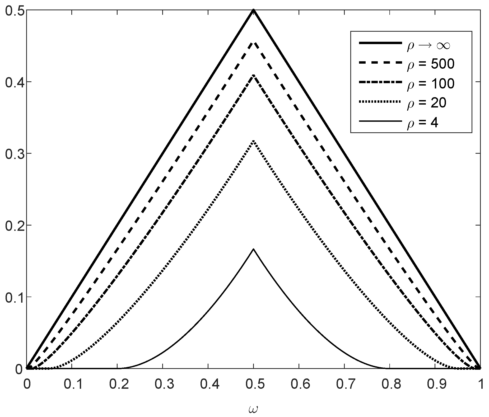
Figure 7 refers to the upper bound on the closeness-to-equiprobable measure $d_{\omega ,n}\left(P_{\ell }\right)$ in (233) for Tunstall trees with n leaves. The bound holds for all $n\in \mathbb{N}$, and it is shown as a function of $\omega \in [0,1]$ for several values of $\rho \in [1,\infty ]$. In the limit where $\rho \to \infty$, the upper bound is equal to $min\{\omega ,1-\omega \}$ since the minimum a-posteriori error probability of the Bayesian binary hypothesis testing model in (228) tends to zero. On the other hand, if $\rho =1$, then the right side of (233) is identically equal to zero (since ${\varphi }_{\omega }\left(1\right)=0$).

Theorem 14 gives an upper bound on the measure in (231), for the closeness of the probability mass function generated on the leaves by a Tunstall tree to the equiprobable distribution, where this bound is expressed as a function of the minimal probability mass of the source. The following result, which relies on ([33], Theorem 4) and our earlier analysis related to Theorem 7, provides a sufficient condition on the minimal probability mass for asserting the closeness of the compression rate to the Shannon entropy of a stationary and memoryless discrete source.

Theorem 15.

Let P be a probability mass function of a stationary and memoryless discrete source, and let the emitted source symbols be from an alphabet of size $D\ge 2$. Let $\mathcal{C}$ be a Tunstall code which is used for source compression; let m and $\mathcal{X}$ denote, respectively, the fixed length and the alphabet of the codewords of $\mathcal{C}$ (where $\left|\mathcal{X}\right|\ge 2$), referring to a Tunstall tree of n leaves with $n\le {\left|\mathcal{X}\right|}^m<n+(D-1)$. Let $p_{min}$ be the minimal probability mass of the source symbols, and let

$$d=d(m,\epsilon ):=\{\begin{array}{cc}\frac{m\epsilon {log}_{\mathrm{e}}\left|\mathcal{X}\right|}{1+\epsilon }+{log}_{\mathrm{e}}\left(1-\frac{D-1}{{\left|\mathcal{X}\right|}^m}\right),\hfill & if D>2,\hfill \\ \frac{m\epsilon {log}_{\mathrm{e}}\left|\mathcal{X}\right|}{1+\epsilon },\hfill & if D=2,\hfill \end{array}$$

(235)

with an arbitrary $\epsilon >0$ such that $d>0$. If

$$\begin{array}{c}\hfill p_{min}\ge \frac{W_0\left(-{\mathrm{e}}^{-d-1}\right)}{W_{-1}\left(-{\mathrm{e}}^{-d-1}\right)},\end{array}$$

(236)

where $W_0$ and $W_{-1}$ denote, respectively, the principal and secondary real branches of the Lambert W function [37], then the compression rate of the Tunstall code is larger than the Shannon entropy of the source by a factor which is at most $1+\epsilon$.

Proof. 

See Appendix P.2.  □

Remark 13.

The condition in (236) can be replaced by the stronger requirement that

$$\begin{array}{c}\hfill p_{min}\ge \frac{1}{1+\sqrt{8d}}.\end{array}$$

(237)

Unless d is a small fraction of unity, there is a significant difference between the condition in (236) and the more restrictive condition in (237) (see Figure 8).

Example 3.

Consider a memoryless and stationary binary source, and a binary Tunstall code with codewords of length $m=10$ referring to a Tunstall tree with $n=2^m=1024$ leaves. Letting $\epsilon =0.1$ in Theorem 15, it follows that if the minimal probability mass of the source satisfies $p_{min}\ge 0.0978$ (see (235), and Figure 8 with $d=\frac{m\epsilon {log}_{\mathrm{e}}2}{1+\epsilon }=0.6301$), then the compression rate of the Tunstall code is at most $10\%$ larger than the Shannon entropy of the source.

References

1. Ali, S.M.; Silvey, S.D. A general class of coefficients of divergence of one distribution from another. J. R. Stat. Soc. 1966, 28, 131–142. [Google Scholar] [CrossRef]
2. Csiszár, I. Eine Informationstheoretische Ungleichung und ihre Anwendung auf den Bewis der Ergodizität von Markhoffschen Ketten. Publ. Math. Inst. Hungar. Acad. Sci. 1963, 8, 85–108. (In German) [Google Scholar]
3. Csiszár, I. A note on Jensen’s inequality. Studia Scientiarum Mathematicarum Hungarica 1966, 1, 185–188. [Google Scholar]
4. Csiszár, I. Information-type measures of difference of probability distributions and indirect observations. Studia Scientiarum Mathematicarum Hungarica 1967, 2, 299–318. [Google Scholar]
5. Csiszár, I. On topological properties of f-divergences. Studia Scientiarum Mathematicarum Hungarica 1967, 2, 329–339. [Google Scholar]
6. Csiszár, I. A class of measures of informativity of observation channels. Periodica Mathematicarum Hungarica 1972, 2, 191–213. [Google Scholar] [CrossRef]
7. Morimoto, T. Markov processes and the H-theorem. J. Phys. Soc. Jpn. 1963, 18, 328–331. [Google Scholar] [CrossRef]
8. Liese, F.; Vajda, I. Convex Statistical Distances. In Teubner-Texte Zur Mathematik; Springer: Leipzig, Germany, 1987; Volume 95. [Google Scholar]
9. Pardo, L. Statistical Inference Based on Divergence Measures; Chapman and Hall/CRC, Taylor &amp, Ed.; Francis Group: Boca Raton, FL, USA, 2006. [Google Scholar]
10. Pardo, M.C.; Vajda, I. About distances of discrete distributions satisfying the data processing theorem of information theory. IEEE Trans. Inf. Theory 1997, 43, 1288–1293. [Google Scholar] [CrossRef]
11. Stummer, W.; Vajda, I. On divergences of finite measures and their applicability in statistics and information theory. Statistics 2010, 44, 169–187. [Google Scholar] [CrossRef]
12. Vajda, I. Theory of Statistical Inference and Information; Kluwer Academic Publishers: Dordrecht, The Netherlands, 1989. [Google Scholar]
13. Ziv, J.; Zakai, M. On functionals satisfying a data-processing theorem. IEEE Trans. Inf. Theory 1973, 19, 275–283. [Google Scholar] [CrossRef]
14. Zakai, M.; Ziv, J. A generalization of the rate-distortion theory and applications. In Information Theory—New Trends and Open Problems; Longo, G., Ed.; Springer: Berlin/Heidelberg, Germany, 1975; pp. 87–123. [Google Scholar]
15. Merhav, N. Data processing theorems and the second law of thermodynamics. IEEE Trans. Inf. Theory 2011, 57, 4926–4939. [Google Scholar] [CrossRef]
16. Liese, F.; Vajda, I. On divergences and informations in statistics and information theory. IEEE Trans. Inf. Theory 2006, 52, 4394–4412. [Google Scholar] [CrossRef]
17. Csiszár, I.; Körner, J. Information Theory: Coding Theorems for Discrete Memoryless Systems, 2nd ed.; Cambridge University Press: Cambridge, UK, 2011. [Google Scholar]
18. Ahlswede, R.; Gács, P. Spreading of sets in product spaces and hypercontraction of the Markov operator. Ann. Probab. 1976, 4, 925–939. [Google Scholar] [CrossRef]
19. Calmon, F.P.; Polyanskiy, Y.; Wu, Y. Strong data processing inequalities for input constrained additive noise channels. IEEE Trans. Inf. Theory 2018, 64, 1879–1892. [Google Scholar] [CrossRef]
20. Cohen, J.E.; Iwasa, Y.; Rautu, Gh.; Ruskai, M.B.; Seneta, E.; Zbăganu, G. Relative entropy under mappings by stochastic matrices. Linear Algebra Appl. 1993, 179, 211–235. [Google Scholar] [CrossRef] [Green Version]
21. Cohen, J.E.; Kemperman, J.H.B.; Zbăganu, Gh. Comparison of Stochastic Matrices with Applications in Information Theory, Statistics, Economics and Population Sciences; Birkhäuser: Boston, MA, USA, 1998. [Google Scholar]
22. Makur, A.; Polyanskiy, Y. Comparison of channels: Criteria for domination by a symmetric channel. IEEE Trans. Inf. Theory 2018, 64, 5704–5725. [Google Scholar] [CrossRef]
23. Polyanskiy, Y.; Wu, Y. Dissipation of information in channels with input constraints. IEEE Trans. Inf. Theory 2016, 62, 35–55. [Google Scholar] [CrossRef]
24. Raginsky, M. Strong data processing inequalities and Φ-Sobolev inequalities for discrete channels. IEEE Trans. Inf. Theory 2016, 62, 3355–3389. [Google Scholar] [CrossRef]
25. Polyanskiy, Y.; Wu, Y. Strong data processing inequalities for channels and Bayesian networks. In Convexity and Concentration; Carlen, E., Madiman, M., Werner, E.M., Eds.; Springer: Berlin/Heidelberg, Germany, 2017; Volume 161, pp. 211–249. [Google Scholar]
26. Makur, A.; Zheng, L. Linear bounds between contraction coefficients for f-divergences. arXiv 2018, arXiv:1510.01844.v4. [Google Scholar]
27. Pearson, K. On the criterion that a given system of deviations from the probable in the case of a correlated system of variables is such that it can be reasonably supposed to have arisen from random sampling. Lond. Edinb. Dublin Philos. Mag. J. Sci. 1900, 50, 157–175. [Google Scholar] [CrossRef]
28. Neyman, J. Contribution to the theory of the χ2 test. In Proceedings of the First Berkeley Symposium on Mathematical Statistics and Probability, Berkeley, CA, USA, 13–18 August 1945 and 27–29 January 1946; University of California Press: Berkeley, CA, USA, 1949; pp. 239–273. [Google Scholar]
29. Sarmanov, O.V. Maximum correlation coefficient (non-symmetric case). In Selected Translations in Mathematical Statistics and Probability; American Mathematical Society: Providence, RI, USA, 1962. [Google Scholar]
30. Marshall, A.W.; Olkin, I.; Arnold, B.C. Inequalities: Theory of Majorization and Its Applications, 2nd ed.; Springer: Berlin/Heidelberg, Germany, 2011. [Google Scholar]
31. Steele, J.M. The Cauchy-Schwarz Master Class; Cambridge University Press: Cambridge, UK, 2004. [Google Scholar]
32. Bhatia, R. Matrix Analysis; Springer: Berlin/Heidelberg, Germany, 1997. [Google Scholar]
33. Cicalese, F.; Gargano, L.; Vaccaro, U. Bounds on the entropy of a function of a random variable and their applications. IEEE Trans. Inf. Theory 2018, 64, 2220–2230. [Google Scholar] [CrossRef]
34. Sason, I. Tight bounds on the Rényi entropy via majorization with applications to guessing and compression. Entropy 2018, 20, 896. [Google Scholar] [CrossRef]
35. Ho, S.W.; Verdú, S. On the interplay between conditional entropy and error probability. IEEE Trans. Inf. Theory 2010, 56, 5930–5942. [Google Scholar] [CrossRef]
36. Ho, S.W.; Verdú, S. Convexity/concavity of the Rényi entropy and α-mutual information. In Proceedings of the 2015 IEEE International Symposium on Information Theory, Hong Kong, China, 14–19 June 2015; pp. 745–749. [Google Scholar]
37. Corless, R.M.; Gonnet, G.H.; Hare, D.E.G.; Jeffrey, D.J.; Knuth, D.E. On the Lambert W function. Adv. Comput. Math. 1996, 5, 329–359. [Google Scholar] [CrossRef]
38. Cicalese, F.; Gargano, L.; Vaccaro, U. A note on approximation of uniform distributions from variable-to-fixed length codes. IEEE Trans. Inf. Theory 2006, 52, 3772–3777. [Google Scholar] [CrossRef]
39. Tsallis, C. Possible generalization of the Boltzmann-Gibbs statistics. J. Stat. Phys. 1988, 52, 479–487. [Google Scholar] [CrossRef]
40. Rényi, A. On measures of entropy and information. In Proceedings of the Fourth Berkeley Symposium on Mathematical Statistics and Probability, Berkeley, CA, USA, 20 June–30 July 1960; University of California Press: Berkeley, CA, USA, 1961; Volume 1, pp. 547–561. [Google Scholar]
41. Cicalese, F.; Gargano, L.; Vaccaro, U. Minimum-entropy couplings and their applications. IEEE Trans. Inf. Theory 2019, 65, 3436–3451. [Google Scholar] [CrossRef]
42. Sason, I.; Verdú, S. Arimoto-Rényi conditional entropy and Bayesian M-ary hypothesis testing. IEEE Trans. Inf. Theory 2018, 64, 4–25. [Google Scholar] [CrossRef]
43. Amari, S.; Nagaoka, H. Methods of Information Geometry; Oxford University Press: New York, NJ, USA, 2000. [Google Scholar]
44. Cichocki, A.; Amari, S.I. Families of Alpha- Beta- and Gamma- divergences: Flexible and robust measures of similarities. Entropy 2010, 12, 1532–1568. [Google Scholar] [CrossRef]
45. Sason, I. On f-divergences: Integral representations, local behavior, and inequalities. Entropy 2018, 20, 383. [Google Scholar] [CrossRef]
46. Fano, R.M. Class Notes for Course 6.574: Transmission of Information; MIT: Cambridge, MA, USA, 1952. [Google Scholar]
47. Ahlswede, R.; Gács, P.; Körner, J. Bounds on conditional probabilities with applications in multi-user communication. Z. Wahrscheinlichkeitstheorie verw. Gebiete 1977, 34, 157–177, Correction in 1977, 39, 353–354. [Google Scholar] [CrossRef]
48. Raginsky, M.; Sason, I. Concentration of measure inequalities in information theory, communications and coding: Third edition. In Foundations and Trends (FnT) in Communications and Information Theory; NOW Publishers: Delft, The Netherlands, 2019; pp. 1–266. [Google Scholar]
49. Chen, X.; Guntuboyina, A.; Zhang, Y. On Bayes risk lower bounds. J. Mach. Learn. Res. 2016, 17, 7687–7744. [Google Scholar]
50. Guntuboyina, A. Lower bounds for the minimax risk using f-divergences, and applications. IEEE Trans. Inf. Theory 2011, 57, 2386–2399. [Google Scholar] [CrossRef]
51. Kim, Y.H.; Sutivong, A.; Cover, T.M. State amplification. IEEE Trans. Inf. Theory 2008, 54, 1850–1859. [Google Scholar] [CrossRef]
52. Arimoto, S. Information measures and capacity of order α for discrete memoryless channels. In Topics in Information Theory—2nd Colloquium; Csiszár, I., Elias, P., Eds.; Colloquia Mathematica Societatis Janós Bolyai; Elsevier: Amsterdam, The Netherlands, 1977; Volume 16, pp. 41–52. [Google Scholar]
53. Ahlswede, R.; Körner, J. Source coding with side information and a converse for degraded broadcast channels. IEEE Trans. Inf. Theory 1975, 21, 629–637. [Google Scholar] [CrossRef]
54. Liu, J.; Cuff, P.; Verdú, S. Eγ resolvability. IEEE Trans. Inf. Theory 2017, 63, 2629–2658. [Google Scholar]
55. Brémaud, P. Discrete Probability Models and Methods: Probability on Graphs and Trees, Markov Chains and Random Fields, Entropy and Coding; Springer: Basel, Switzerland, 2017. [Google Scholar]
56. Tunstall, B.K. Synthesis of Noiseless Compression Codes. Ph.D. Thesis, Georgia Institute of Technology, Atlanta, GA, USA, 1967. [Google Scholar]
57. DeGroot, M.H. Uncertainty, information and sequential experiments. Ann. Math. Stat. 1962, 33, 404–419. [Google Scholar] [CrossRef]
58. Roberts, A.W.; Varberg, D.E. Convex Functions; Academic Press: Cambridge, MA, USA, 1973. [Google Scholar]
59. Rockafellar, R.T. Convex Analysis; Princeton University Press: Princeton, NJ, USA, 1996. [Google Scholar]
60. Collet, J.F. An exact expression for the gap in the data processing inequality for f-divergences. IEEE Trans. Inf. Theory 2019, 65, 4387–4391. [Google Scholar] [CrossRef]
61. Bregman, L.M. The relaxation method of finding the common points of convex sets and its application to the solution of problems in convex programming. USSR Comput. Math. Math. Phys. 1967, 7, 200–217. [Google Scholar] [CrossRef]
62. Sason, I.; Verdú, S. f-divergence inequalities. IEEE Trans. Inf. Theory 2016, 62, 5973–6006. [Google Scholar] [CrossRef]
63. Gilardoni, G.L. On Pinsker’s and Vajda’s type inequalities for Csiszár’s f-divergences. IEEE Trans. Inf. Theory 2010, 56, 5377–5386. [Google Scholar] [CrossRef]
64. Gibbs, A.L.; Su, F.E. On choosing and bounding probability metrics. Int. Stat. Rev. 2002, 70, 419–435. [Google Scholar] [CrossRef]
65. Simic, S. Second and third order moment inequalities for probability distributions. Acta Math. Hung. 2018, 155, 518–532. [Google Scholar] [CrossRef]
66. Van Erven, T.; Harremoës, P. Rényi divergence and Kullback–Leibler divergence. IEEE Trans. Inf. Theory 2014, 60, 3797–3820. [Google Scholar] [CrossRef]
67. Pardo, M.C.; Vajda, I. On asymptotic properties of information-theoretic divergences. IEEE Trans. Inf. Theory 2003, 49, 1860–1868. [Google Scholar] [CrossRef]
68. Beck, A. Introduction to Nonlinear Optimization: Theory, Algorithms and Applications with Matlab; SIAM-Society for Industrial and Applied Mathematics: Philadelphia, PA, USA, 2014. [Google Scholar]
69. Simic, S. On logarithmic convexity for differences of power means. J. Inequalities Appl. 2008, 2007, 037359. [Google Scholar] [CrossRef]
70. Keziou, A. Dual representation of φ-divergences and applications. C. R. Math. 2003, 336, 857–862. [Google Scholar] [CrossRef]
71. Nguyen, X.; Wainwright, M.J.; Jordan, M.I. Estimating divergence functionals and the likelihood ratio by convex risk minimization. IEEE Trans. Inf. Theory 2010, 56, 5847–5861. [Google Scholar] [CrossRef]
72. Jelineck, F.; Schneider, K.S. On variable-length-to-block coding. IEEE Trans. Inf. Theory 1972, 18, 765–774. [Google Scholar] [CrossRef]
Figure 1. The bounds in Theorem 2 applied to D f α ( R X n ( λ ) Q X n ) D f α ( R Y n ( λ ) Q Y n ) (vertical axis) versus λ [ 0 , 1 ] (horizontal axis). The f α -divergence refers to Theorem 5. The probability mass functions P X n and Q X n correspond, respectively, to discrete memoryless sources emitting n i.i.d. Bernoulli ( p ) and Bernoulli ( q ) symbols; the symbols are transmitted over BSC ( δ ) with ( α , p , q , δ ) = 1 , 1 4 , 1 2 , 0.110 . The bounds in the upper and middle plots are compared to the exact values, being computationally feasible for n = 1 and n = 10 , respectively. The upper, middle and lower plots correspond, respectively, to n = 1 , n = 10 , and n = 50 .
Entropy 21 01022 g001
Figure 2. The upper bound in Theorem 4 applied to D f α ( R Y n ( λ ) Q Y n ) D f α ( R X n ( λ ) Q X n ) (see (125)–(127)) in the vertical axis versus λ [ 0 , 1 ] in the horizontal axis. The f α -divergence refers to Theorem 5. The probability mass functions P X i and Q X i are Bernoulli ( p ) and Bernoulli ( q ) , respectively, for all i { 1 , , n } with n uses of BSC ( δ ) , and parameters ( p , q , δ ) = 1 4 , 1 2 , 0.110 . The upper and middle plots correspond to n = 10 with α = 10 and α = 100 , respectively; the middle and lower plots correspond to α = 100 with n = 10 and n = 100 , respectively. The bounds in the upper and middle plots are compared to the exact values, being computationally feasible for n = 10 .
Entropy 21 01022 g002
Figure 3. Plots of d f α ( p q ) , its upper and lower bounds in (61) and (65), respectively, and its asymptotic approximation in (66) for large values of α . The plots are shown as a function of α e 3 2 , 1000 . The upper and lower plots refer, respectively, to ( p , q ) = ( 0.1 , 0.9 ) and ( p , q ) = ( 0.2 , 0.8 ) .
Entropy 21 01022 g003
Figure 4. Curves of the upper bound on the ratio of contraction coefficients μ f α ( Q X , W Y | X ) μ χ 2 ( Q X , W Y | X ) (see the right-side inequality of (130)) as a function of the parameter α e 3 2 . The curves correspond to different values of ξ in (131).
Entropy 21 01022 g004
Figure 5. A comparison of the maximal values of ρ (minus 1) according to (171) and (172), asserting the satisfiability of the condition D ( Q U n ) d log e , with an arbitrary d > 0 , for all integers n 2 and probability mass functions Q supported on { 1 , , n } with q max q min ρ . The solid line refers to the necessary and sufficient condition which gives (171), and the dashed line refers to a stronger condition which gives (172).
Entropy 21 01022 g005
Figure 6. A comparison of the exact expression of Φ ( α , ρ ) in (175), with α = 1 , and its three upper bounds in the right sides of (176), (177) and (180) (called ’Upper bound 1’ (dotted line), ’Upper bound 2’ (thin dashed line), and ’Upper bound 3’ (thick dashed line), respectively).
Entropy 21 01022 g006
Figure 7. Curves of the upper bound on the measure d ω , n ( P ) in (233), valid for all n N , as a function of ω [ 0 , 1 ] for different values of ρ : = 1 p min .
Entropy 21 01022 g007
Figure 8. Curves for the smallest values of p min , in the setup of Theorem 15, according to the condition in (236) (solid line) and the more restrictive condition in (237) (dashed line) for binary Tunstall codes which are used to compress memoryless and stationary binary sources.
Entropy 21 01022 g008